

Validation of Remotely Sensed Land Surface Temperature at Lake Baikal’s Surroundings Using In Situ Observations

1
Institute of Monitoring of Climatic and Ecological System, Siberian Branch Russian Academy of Sciences, Tomsk 634055, Russia
2
Laboratory of Ecosystem-Atmosphere Interactions in Forest-Bog Complexes, Yugra State University, Khanty-Mansiysk 628012, Russia
3
V. B. Sochava Institute of Geography, Siberian Branch Russian Academy of Sciences, Irkutsk 664033, Russia
*
Author to whom correspondence should be addressed.
Land 2024, 13(4), 555; https://doi.org/10.3390/land13040555
Submission received: 4 March 2024
/
Revised: 15 April 2024
/
Accepted: 19 April 2024
/
Published: 21 April 2024
(This article belongs to the Special Issue Digital Mapping for Ecological Land)
Abstract
:The accuracy of Land Surface Temperature (LST) products retrieved from satellite data in mountainous-coastal areas is not well understood. This study presents an analysis of the spatial and temporal variability of the differences between the LST and in situ observed air and surface temperatures (ISTs) for the southeastern slope of Lake Baikal’s surroundings. The IST was measured at 12 ground observation sites located on the southeastern macro-slope of the Primorskiy Ridge (Baikal, Russia) within an elevation range of 460–1656 m above sea level from 2009 to 2021. LST was estimated using 617 Landsat (7 and 8) images from 2009–2021, taking into account brightness temperature, surface emissivity and vegetation cover fraction. The comparison of the LST from satellite data and the IST from ground observation showed relatively high differences, which varied depending on the season and site type. A neural network was suggested and calibrated to improve the LST data. The corrected remote-sensed temperature was found to reproduce the IST very well, with mean differences of about 0.03 °C and linear correlation coefficients of 0.98 and 0.95 for the air and surface IST.
1. Introduction
Land surface temperature (LST) is a complex physical-geographic characteristic that is in high demand for the investigation of processes in the Earth’s system [1,2]. Analysis of LST is used in various areas, including the study of local, regional or global climate changes at urban or agricultural regions, energy balance, hydrology, etc. [3,4,5,6,7,8,9].
Various techniques are being developed for calculating LST from remote-acquired satellite or aerial images [10]. A number of remote systems are shooting in the thermal range (MODIS, AVHRR, AATSR, SEVIRI, Landsat, etc.). The remote systems obtain an averaged radiative temperature for a certain image pixel and a specific spectral range [11]. The outgoing radiation recorded in the satellite images depends on the surface temperature and emissivity. There are also many maps of the global level of generalization created on the basis of satellite imagery and reflecting the LST [12]. Much attention has been paid to the correctness of the satellite-retrieved data. In 2012, the international network Earthtemp Network [13] was created, which brings together scientists who are studying the Earth’s surface temperature and developing methods for its calculation. The organization focuses on the comparison of ground and remote data [14].
Notable distortions and imprecisions at converting thermal image brightness characteristics into temperature values occur when the surface emissivity is not taken into account. It is especially relevant for land surfaces due to the varying emissivity of different landscape types such as bare soil, grass, and forests. Moreover, distinct microclimates with varying temperature regimes are present in different landscapes. The satellite images record the temperature of the surface layer (soil in open areas, grass cover in meadow areas, tree crowns in the forest, snow surfaces in winter), which must be taken into account when developing an algorithm for calculating air and surface temperature using satellite images.
A large number of studies are devoted to comparing data from weather stations, as well as other ground-based (in situ) observations and remote data on land air and land surface temperature (LAT and LST, respectively) including determining their validations, accuracy assessments, identification inconsistencies, surface emissivities, etc. [15,16]. The data of ground-based temperature observations are considered accurate and are used to validate the remote data [17,18,19,20].
Air temperature is a crucial meteorological parameter that affects local biological and physical processes. It is measured at weather stations worldwide at 2 m above the surface. The mean global air temperature is a significant variable in describing global climatic changes. The LST from satellite data is different from surface or air temperature measured locally. Understanding the relationship between remotely sensed LST and contact-measured air temperature enables the conversion of different temperature characteristics into a single scale. This allows for the analysis of the spatial variability of a microclimate.
Satellite-derived LAT and LST are highly correlated values but are controlled by a differing set of land and atmosphere conditions [21], including orography parameters (elevation, slope and aspect of the surface) and surface energy balance [15,22,23]. Land vegetation is important for temperature formation through the absorption and dissipation of solar radiation, evapotranspiration and changes in surface roughness by influencing sensible heat fluxes and evapotranspiration [24,25]. Atmospheric conditions (i.e., precipitable water vapour) should also be accounted for in the LST calculation using the remote data [20,26].
In recent decades, various methods for improving the performance of remotely sensed LSTs have been widely applied [3]. These methods include accounting for the relationship with physiographic variables [27], the radiometric cross-calibration of satellite data [28] and various statistical methods (linear/nonlinear regression, machine learning methods, random forest and artificial neural networks) [4,29,30].
The study area is located at Lake Baikal, which is listed as a UNESCO World Heritage Site. Our research was conducted in the Central Ecological Zone of the Baikal Natural Area, which is a specially protected area that includes the Pribaikalsky National Park. Air temperature is a crucial component in calculating hydrothermal coefficients, bioclimatic indices, and other variables. Changes in air temperature in the natural landscapes of the Baikal natural territory occur synchronously with global ones. However, due to the influence of Lake Baikal, they are smoother than the global air temperature changes. To evaluate the sensitivity of landscape components to current changes, we need to know the trends of these changes, which cannot be obtained using only local measurement data. The study area has a limited number of weather stations, which are only located on the coastal territory. Our microclimatic observations covered various landscapes, from the coast to the mountains. We have monitoring sites located along the profile at altitudes ranging from 460 to 1656 m above sea level. To obtain a comprehensive picture of soil and air temperature distribution, we need to incorporate other data sources and use multilevel models.
The aim of this study is to analyse the spatial and temporal variability of the differences between the land surface temperature (LST) and the air and surface temperatures observed in situ. The relationships between the LST and orographic, vegetation and atmospheric conditions were used to improve the representation of observed temperatures from satellite data. In situ temperature monitoring was conducted in a mountainous area on the west shore of Lake Baikal. The focus of this study is related to two issues. The first task was to test the accuracy of the LST calculation algorithm from the Landsat satellite images using in situ observations in a mountainous area in the Siberian region. The second task involveed using a neural network approach to correct the LST data obtained from satellite images.
2. Materials and Methods
2.1. Study Area
The study area is located in the surroundings of Lake Baikal (central point: 53°02′46.1″ N 106°45′37.3″ E). It extends from the Sarminsky Golets mountain to the shoreline of Lake Baikal at the Baikal-facing macro-slope of the Primorskiy Ridge (Figure 1). The topography of the area is primarily influenced by a long bench known as the Obruchevskii fault, which runs along the Primorskiy Ridge. This fault showcases a combination of Archean and Lower Proterozoic rock formations. Study area landscapes are typical for the Baikal–Dzhugdzhur mountain taiga region and the Baikal mountain and taiga depressions [31]. The altitude-belt landscape structure is formed over the mountain environment of Lake Baikal under the influence of the barrier-shade, arid-depression and submountain effects, accompanied by the waters of Lake Baikal [32]. As a result, a combination of contrasting landscapes is formed, including the Anginsky–Sarminsky middle taiga, a predominantly light coniferous region, the Olkhon mountain-subtaiga, and submountain-steppe landscapes [33].
The local climate is characterized by an anticyclonic type with a lack of atmospheric precipitations. The annual precipitation range is from 100 to 400 mm. The warm season lasts 4–4.5 months. The annual temperature is 0.7 °C; the coldest month is January (−17.3 °C) and the warmest month is July (+14.4 °C) [34].
Climatic changes in the Lake Baikal area are characterized by a stable rise of annual air temperatures (0.2–0.5 °C/10 years). The rates of warming exceed the average rates for the Northern Hemisphere by approximately 10 times. Changes in the annual precipitation are variable and are mostly statistically insignificant [35].
2.2. In Situ Data
In situ temperature measurements were obtained from 12 ground observation sites (see Figure 1, Table 1). The sites were organized on the southeastern macro-slope of the Primorskiy Ridge. The monitoring sites are located in two transects with an elevation range of 460–1656 m above sea level. The first transect (sites P1–P3) passes from the lake shore via the Tazheran Steppe to the middle of the Primorskiy Ridge slope (observations started in 2009). The second transect (sites S1–S9) runs along the slope from Lake Baikal to the highest local mountain Sarminsky Golets, with a height of 1656 m. Photos of observation sites are given at the Supplementary S1.
The study sites were subdivided into open, semi-closed and closed according to the density of the tree-shrub vegetation. The closed sites (S2, S3, S5, P2 and P3 from Table 1) are located in forests with tall tree layers (15–30 m) and crown projective covers of 60–90%. The semi-closed sites (S6, S7, S8, P1) are located in sparse forests with crown projective covers of 20–50% or at the edge of a forest patch. The ground cover at the open sites (S1, S4, S9) is provided by small grasses or bare soil.
The automatic observations of air and soil surface temperature were carried out using Thermochrons—button-sized steel temperature loggers (DS1920L, Dallas Semiconductor Corp., Dallas, TX, USA) [36] that were used for temperature monitoring from 2009 to 2019 [30]. Automatic temperature recorders (Elitech RC-51H and Elitech RC-4HC, London, UK) [37] have been used since 2019. The accuracy of the temperature measurements was 0.5 °C. The automatic temperature recorders were placed at 2 m above the surface at the northern side of a tree. The soil surface temperature measurements were conducted by placing temperature recorders on soil covered by leaves or small herbs to prevent heating from sunlight. Measurements were taken at 1 h intervals. Both the air and soil surface temperatures were registered at each study site. Photos of the equipment are given in Supplementary S2.
2.3. Satellite Data
Methods for the calculation of the LST from space images are developed for estimating the spatial distribution of the Earth’s surface temperature. In total, 617 Landsat (7 and 8) images from 2009–2021 were collected to calculate the LST because their temporal—spatial resolutions correspond to the objectives and scale of the study. The patial resolution for Landsat 7 is 30 m, except for band 6 for Landsat 7, which has 60 m resolution and band 8, which has 15 m resolution (Table 2).
The LST calculations were performed using the Google Earth Engine TM (GEE) [38], which allows the processing of large data massifs on a remote server, as well as an algorithm developed by Ermida et al. [39].
The algorithm uses the atmosphere’s brightness temperatures for the Landsat’s infrared channels, available in GEE as input data. A Statistical Mono-Window algorithm developed by the Climate Monitoring Satellite Application Facility for deriving LST climate data records from Meteosat First and Second Generation [40] was used for atmospheric correction as well as surface emissivity from the ASTER GED v3 dataset [41], the vegetation cover fraction and vegetation index relationship [42] and Vegetation-Cover emissivity calculation [43]. A specific algorithm was used for the fraction of vegetation cover (FVC) calculations [44] on the basis of Landsat data due to the lack of ASTER GEDv3 data.
A detailed description of the LST calculation algorithm is given at [39]. The processing chain includes a selection of the date range, the Landsat satellite and the region of interest to process. The main module applies a cloud mask, computes the NDVI, converts it to a fraction of vegetation cover values and obtains the corresponding Landsat emissivity. Finally, the algorithm is applied to the Landsat thermal infrared band image, taking into account emissivity and the total column water vapor contents [39].
2.4. Comparison of LST and IST
The land surface temperatures for the study sites were extracted from the LST maps calculated with the Google Earth Engine [38]. Only cloud-free conditions were used for point LST estimation at the study sites. The time of the satellite passing over the study area varied from 12:00 to 12:56 p.m. (local time) with a median value of 12:45 p.m. In order to reduce errors related to temperature–temporal variations, in situ hourly temperature data were interpolated to the exact time of a satellite image. The linear interpolation between the hours before and after the satellite’s passing was used for the calculation of the in situ temperature (IST) matched to the LST. The differences between ISTs and LSTs both for air and soil surface temperatures were calculated for all matchups.
The accuracy of the LST was estimated by the median difference (MD), which is the robust estimation, and computed as:
where LST is the temperature derived from satellite data according to the procedure listed in Section 2.3, and IST is the in situ-obtained temperature of the air or soil surface. The robust precision estimation given by the median of absolute residuals (MAR) was calculated as follows:
The root mean squared difference (RMSD) is a characteristic of the total uncertainty:
where N is the number of observations.
The Pearson linear correlation coefficient (R) was computed as an estimate of the time series synchronism.
2.5. Correction of LST Using Artificial Neural Network
A specific procedure of the recalibration satellite that retrieved the LST was suggested to improve the performance of remote-sensed data [3]. The relationship between the LST and the biophysical variables [4,27,29,30,45] allowed us to suggest a correction procedure for the better representation of the IST from satellite data. The correction procedure is based on not obvious links that were simulated by a neural network that is widely used for satellite data processing [7].
A neural network algorithm was used for the simulation of unclear dependencies between remotely sensed parameters and the IST. The Neural Fitting app (MATLAB 2014b) was applied to build and test the artificial neural network. The input parameters of the network include the LST, site elevation, a fraction of the vegetation and the precipitable water amount. The target parameter was the air or surface IST. The full dataset was divided into the training (70%), validation (15%) and test (15%) subsets that were randomly selected from the input vectors and targets. A two-layer feed-forward network was selected for data simulation. The hidden neuron numbers were set to 10. The Levenberg–Marquardt backpropagation algorithm (trainlm) was used to train the network. The network generated corrected the remote-sensed temperature (CRT). Two separate networks were trained using the air IST and the surface IST as target parameters.
3. Results
3.1. Air and Surface Temperature from In-Situ Observations
A time series of daily averaged in situ temperatures is shown in Figure 2. Continuous temperature records were not obtained at any study site due to various equipment malfunctions. However, this does not prevent us from describing general patterns of spatial and temporal temperature distribution during the 12-year observation period. The mean annual air temperature decreased with altitude from 2.8 °C in the lake shore part to −3.3 °C in the sub-nival zone. The average temperature was 0.1 °C on the lake coast due to the maximum impact of the Lake Baikal water body. The distribution of the annual soil surface temperature was influenced by the vegetation type, although, in general, the values were characterized by a decrease with the increase of the site elevation (from 6 °C to −4.2 °C). This type of temperature distribution along the elevation gradient existed in summer. The exception was site S9, where the summer air was colder due to the influence of Lake Baikal. Temperature inversions existed in winter when, due to intensive radiative cooling the lower sites may have been warmer than the upper ones.
The absolute air temperature minimum (−40.7 °C) was observed at site S1 (mnt. Sarminskiy Golets) at 8:00 on 5 February 2019. The absolute maximum (+36.0 °C) for was at site S9 (steppe at Lake Baikal shore) at 17:00 on 19 June 2015 and at 14:00 on 22 July 2015. Soil surface temperatures had higher variabilities in summer with maximal values of +56.2 °C (site S4) at 14:00 on 24 May 2017. The minimal values for soil surface temperature were mild in comparison with the air temperature due to the presence of snow cover in winter. The minimal surface IST was −26.7 °C at site S8 at 8:00 on 29 November 2017.
Vegetation played an important role in both the winter and summer seasons [46]. The temperature regime essentially differed at sites located at similar elevations (site S3—1101 m and site S4—1117 m), where the influence of the elevation factor and the distance from Lake Baikal were similar. The differences in temperature here were caused by various landscape conditions. The landscape at site S3 is presented by cedar–fir–motley herb forests while burned-out birch patches with stone placers are located at site S4. The canopy effectively obstructs the incoming solar radiation, and vegetation transpiration reinforces the cooling effect, which inhibits the rise of surface temperature [15]. The soil surface at site S4 is more open for direct insolation, and the soil warms up better. Hence, the soil and air temperatures at site S4 pass through 0 °C earlier in spring and later in autumn than at site S3. The time of transition of the soil temperature through 0 °C differs by 5–7 days in spring and by 6–27 days in autumn. The dates of stable transition of the surface temperature through 5 °C differ by 40–60 days both in spring and autumn.
The obtained results confirm the described patterns of temperature distribution along the slope of the Primorskiy Range, with the identification of the zone of influence of Lake Baikal at an elevation of 1000 m [47].
3.2. LST from Satellite
Figure 3 shows an example of the LST calculated from a satellite image acquired on 24 July 2014. Some clouds exist at the northeast part of the image. Generally, three large areas with significantly different temperatures can be recognized in the image. The first area is the cold surface of Lake Baikal with the LST about 14–16 °C at the main body and 20 °C at the Maloe More Strait. The second area is related to the Tazheranskaya steppe and Olkhon Island. Bare soil, rocks and thinned grass cover warmed up to 35–42 °C under direct sun conditions. Lake Baikal’s shore in the northeast part of the image is also heated to 35–40 °C due to the south slope orientation and steppe landscapes. The northwest part of the territory has a land temperature from 16 to 30 °C approximately and is presented by mountains and taiga landscapes.
In total, 617 satellite images were selected for the study area as suitable for LST calculation. Three hundred and thirty-five images were acquired from the Landsat 7 satellite from 2009–2021 and 282 images from Landsat 8 from 2013–2021. The LST point data were collected from LST maps for ground points matched to in situ observations. The whole set of LST data consist of 2347 temperature records. Only 83 LST records were obtained before 2013 from 73 satellite images from Landsat 7. None of the satellite images were found for December. Lake Baikal in midwinter is not yet frozen, has elevated evaporation from open water and forms local cloud cover or haze. The LST at the study sites varied from −32.6 and 46.6 °C. A time series of LST for ground observation sites are shown at Figure 4. The annual course of LST is clearly shown. On average, low elevated sites usually have a higher LST for both winter and summer, but temporal variability is very high. The mean and median LSTs for all sites were 12.1 and 16.2 °C, with a standard deviation of 16.8 °C. The mean temperature values do not correspond to long-term average temperature due to accounting for only the midday temperature (at the moment of satellite passage), which in most cases is the maximum of the measured temperatures for the whole day.
3.3. Validation of LST against IST
A number of in situ observations collected at the moments of the satellite passing were analysed. The in situ air temperature and in situ soil surface temperature differences with the LST were studied (LST–IST). The statistical characteristics for differences between LSTs and ISTs are shown in Table 3. Each study site was used for both air and surface temperature IST measurements. The median difference for the air IST was 3.3 °C and was 1.7 times higher than for the surface IST (2.0 °C). The standard deviation for the whole samples for surface IST difference was a bit higher than for the air IST. Maximal differences, both positive and negative, were obtained for the surface IST. The correlation between in situ and remote-sensed temperatures was good (0.93 and 0.89 for the air and surface IST, respectively), but it was related to the regular annual variation of temperature.
The difference between the LST and the IST should not be recognized as an error of remote sensing observations of the LST due to the varied nature of the measured temperatures. The temperature measured in situ is air temperature or surface temperature regardless of the presence and density of aboveground vegetation cover. The study sites include sites with dense tree cover, with sparse trees and without any trees. The LST measured from the satellite was a radiative temperature corresponding to the emissivity of the specific top of a surface. The LST for a dense forest site will characterize the radiative temperature of the trees’ crown tops, while the air temperature within a forest canopy will be lower in summer and higher in winter. Open surfaces are more suitable for the direct comparison of the satellite-derived LST and the surface IST.
The differences between the LST and the IST vary in both time and space. Figure 5 shows the median difference between the LST and the IST for the individual months of the study period. On average, the MD between the air IST and the LST was about zero or a small negative from November to March. The MD in February was −2.5 °C with a corresponding MAR equal to 1.9 °C and a correlation coefficient of 0.85. The MD for the air IST from April to October was positive and higher by modulus than for the winter months. The largest difference for the air IST was 9.3 °C in May with MAR = 4.5 °C and R = 0.47.
The soil surface temperature in winter was measured under snow cover. The surface IST in winter was significantly higher than the LST. It resulted in a negative MD for the surface IST from November to February. The average January MD was −5.6 °C with a MAR of 4.8 °C and a negligibly small correlation coefficient (~0.001). A positive MD for the surface IST was observed from May to October. A maximal difference (8.1 °C) was found in May with a MAR of 3.9 °C and a correlation coefficient of 0.63.
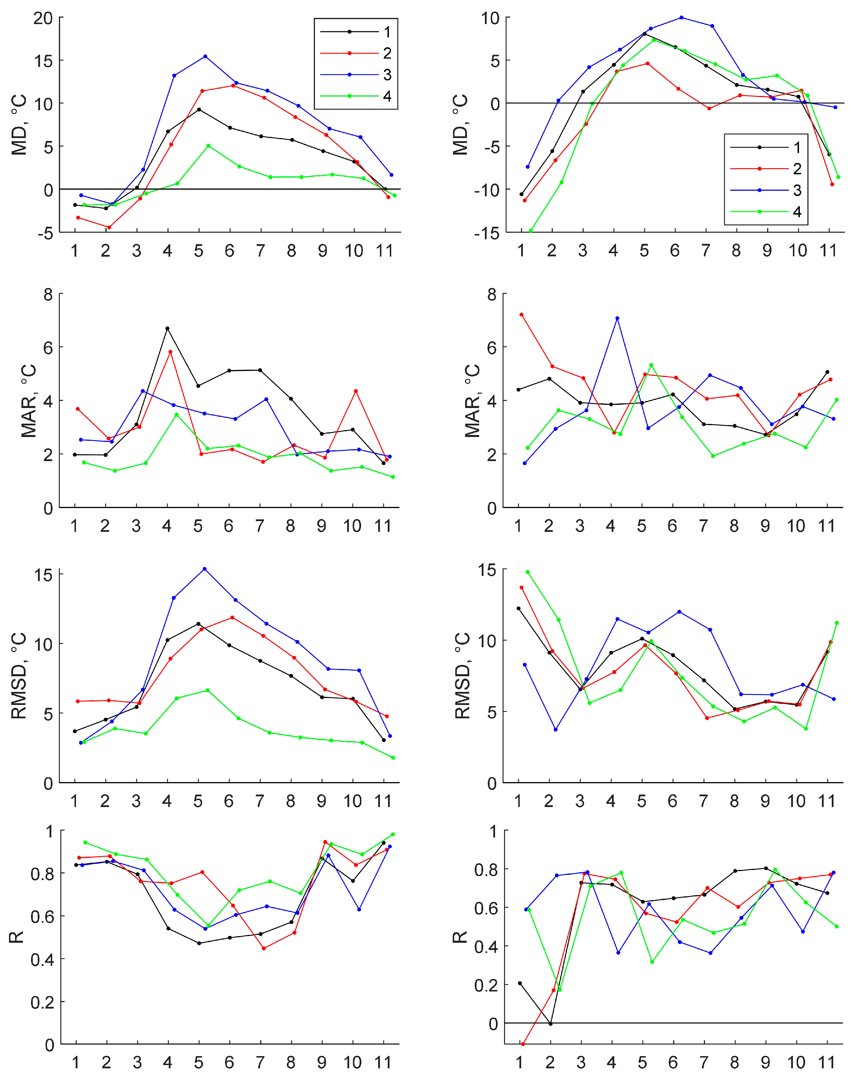
The study sites were subdivided into open, semi-closed and closed according to the density of tall vegetation cover (see Section 2.1). The disagreement of the LST and the IST was related to the degree of shading of the in situ temperature sensor (Figure 6). The colour curves (lines 2–4) represent statistical characteristics for open sites (red line), semi-closed sites (blue line) and closed sites (green line). The black line in Figure 6 corresponds to the characteristics for a whole set of in situ data. The MD for the air ISTs at open and semi-closed sites is larger compared to the closed sites. From April to September, the air MD at open and semi-closed sites exceeded 5.1 °C, reaching 15.4 °C in May at semi-closed sites. While the air MD at the closed sites in May was 5.04 °C, it was less than 2.6 °C during all other months. In wintertime (November–February), the air IST differences were negative. The largest negative differences (−4.5 °C) were observed during February at the open sites. The median absolute residuals for the air ISTs were largest during April and October at the open sites and during the summer months at the semi-closed sites. The closed sites had smaller MARs and RMSDs and a better correlation between the air IST and the LST. The linear correlation coefficient from September to March was higher than for the summer months for all types of sites. A high correlation (R = 0.75–0.94) existed between the air IST and the LST for the open sites except from June–August (R = 0.45–0.65).
The difference between LST and soil surface IST was negative from November to February (Figure 6 right). The largest negative MD (−14.4 °C) was observed for closed sites in January. The largest positive MD for surface was 10.1 °C in June at semi-closed sites. The open sites surface IST is most closely related to the satellite derived LST during the snow-free period that is confirmed by the lowest MD and highest correlation coefficients.
Scatter plots of all match-ups for air and surface IST are presented in Figure 7 to demonstrate an uncertainty of the LST estimations. These show that for negative LST, the difference for air IST is small and LST reasonably reproduces air IST for all types of sites. Air IST difference at positive temperatures rises up to 22 °C for semi-closed sites. The difference remains relatively low (up to 13.8 °C) for closed sites only. Surface IST is linearly related with remote-sensed LST only during the warm season, bur dispersion of IST is high. Closed sites have smaller values of difference between LST and IST at positive LST compared to open and semi-closed sites. Surface IST during winter when the ground is covered by snow falls down to −20.9 °C and −14.7 °C for open and closed sites. The minimal LST was −32.6 °C and −28.9 °C. Snow cover prevents deep cooling of the soil. Hence, the LST and surface IST difference rises with the LST decrease almost linearly.
3.4. Using a Neural Network to Improve LST
The results of direct comparison of the IST and LST show essential differences for both air and surface temperatures. The difference changes throughout a year and from site to site. An artificial neural network was applied for the LST time series to correct it. Two separate networks were trained using the air IST and the surface IST as target parameters.
Corrected remote-sensed temperatures (CRT) were compared against the IST according to the same procedure used for the LST. Table 4 shows the statistical characteristics for differences between the CRT and the IST for air and surface. The CRT reproduces the IST very well. Mean differences were about 0.03 °C and correlations were 0.98 and 0.95 for air and surface ISTs, respectively. The MD became 21 times smaller compared to the MD for the initial LST. Minimal, maximal and median absolute differences also reduced significantly after correction (see Table 2 and Table 3). The RMSE reduced three times for air temperature and about two times for surface temperature.
The monthly MD for the CRT had lower systematic differences in comparison with the MD for theLST (see Figure 5 and Figure 8). The largest mean difference between the air CRT and the air IST was found during January (1.3 °C) and October 1.2 °C). The MD for the surface CRT was a bit higher, with the largest value of 2.2 °C for May. The MD for all other months was less than 1 °C both for the air and surface CRTs. Scatter plots (Figure 9) for the air and surface CRTs show that, after correction using the neural network, the differences of the ISTs do not vary significantly among closed, open and semi-closed sites. A higher negative difference was found for positive surface temperatures at all site types.
A corrected temperature and neural network is suitable only for the dataset used in the present paper, while the suggested approach is applicable for any geographical area if local in situ observations are used for model calibration and testing.
4. Discussion
The direct comparison of near-surface atmospheric temperature with remotely sensed radiative temperature is incorrect due to inherently different forming processes. Solar irradiance heats the Earth’s surface, and the resulting heat flux is distributed in two directions. The downward ground heat flux warms or cools the top soil layers depending on the direction of the heat flux. The upward atmospheric heat flux warms the near-surface air through shortwave radiation reflection or outgoing longwave radiation. The surface temperature and the air temperature are linked through various physical processes, such as longwave radiation, turbulent heat exchange, phase transitions and advection. Our aim is to reconstruct these processes using a neural network approach. In this study, we first converted the radiative temperature obtained from the Landsat satellite into the day land-surface temperature using the GEE module. The temperature was used as input data to estimate the soil surface and air temperatures using neural networks. Corrections were made by comparing the LST with in situ observation data. The modelling results and observation data converged best for the soil surface temperature at open sites. The validation result for air temperature is not ideal, as no model can accurately replicate the intricate physical processes that convert surface temperature into air mass temperature. However, the regularities we have discovered are essential for comprehending natural processes for specialists in geography-related fields such as botany, zoology, landscape science and soil science. This is because in terrains with complex topography, it is not feasible to conduct detailed microclimatic observations to gather data on spatial temperature distribution.
The validation of various satellite data on LST against IST data from ground observations usually shows better performance [1,6,39] than we have found for our sites. The accuracy of LST retrieval for 12 stations across the world using the same algorithm as in the present paper is generally better than 1 °C [39], and the RMSE varies from 1.3 to 3.7 °C. The validation of the LST from the Advanced Baseline Imager [1] using measurements at the 18 sites indicated an overall RMSE of 2.44 °C, a bias of −0.19 °C and an R of 0.99 based on 408,300 data points. The difference (bias), RMSD and R obtained in the present study is higher (Table 3) than reported at [1].
A relatively high mean difference (3.4 °C for the air IST and 2.0 °C for the surface IST) and the RMSD (7.8–7.9 °C) obtained after direct comparison of the LST against the IST makes it difficult to use satellite LST data for a proper description of the local microclimate. Partially high differences are related to local impact of vegetation shading. Better validation results were obtained for the air temperature at open sites in winter when vegetation influence is negligible.
The neural network correction essentially improves the representation of air and surface temperatures from satellite data. The mean difference between the corrected satellite and in situ data becomes almost zero, and the linear correlation coefficients rise to 0.95–0.98. The MAR and RMSD after correction (Table 4) fit ranges obtained in previous studies [1,6,39]. Thestatistical characteristics of the corrected temperatures are close to the ISTs (Figure 10), while LSTs have large biases for TA in summer and TS in winter.
The neural network was trained against in situ observation data and used the LST, site elevation, fraction of vegetation and precipitable water amount as input parameters. The unclear shading impact of vegetation cover on the surface heating was reproduced by the neural network algorithm and led to significant improvement of surface temperature representation from remote-sensed data. A fraction of vegetation cover [39] was a proxy for the estimation of the shading effect.
Correct air and surface temperatures are in high demand for various environmental study applications. The dates of first frost and last frost onset, the dates of vegetation growth start and the sums of active temperatures are calculated using air temperature. Seasonal soil freezing and soil biota activity estimations are used for soil temperature.
5. Conclusions
The objective of this study was to analyse the differences between the LST and the in situ IST in the vicinity of the eastern slope of Lake Baikal, both spatially and temporally. The LST was obtained using Landsat satellite imagery while the IST was measured at 12 sites. The accuracy of the LST was verified using the IST data. Since 2009, small-sized temperature recorders have been used to monitor air and soil surface temperatures, revealing the temperature characteristics of the mountain–taiga–steppe landscapes surrounding Lake Baikal. A vast collection of satellite images was processed to calculate the LST, taking into account top-of-atmosphere brightness temperatures, surface emissivity, and atmospheric water vapor content.
The validation of the matched-up LST from satellite data and the IST from ground observations demonstrated relatively high differences between data. Differences depend on the season and site type. The MDs for the air ISTs at open and semi-closed sites are larger compared to those of closed sites. From April to September, the air MDs at open and semi-closed sites are large and positive. Wintertime (November–February) air IST differences are negative. The largest negative differences (−4.5 °C) were observed in February at open sites. The linear correlation coefficients from September to March are higher than for the summer months for all types of sites. A high correlation (R = 0.75 ÷ 0.94) exists between the air ISTs and the LSTs for open sites, except from June–August (R = 0.45 ÷ 0.65).
A neural network algorithm was calibrated for LST data improvement. Corrected remote-sensed temperature reproduces IST very well. Mean differences are about 0.03 °C, and linear correlations are 0.98 and 0.95 for the air and surface ISTs, respectively. After correction, the difference with IST does not vary significantly between closed, open and semi-closed sites. Higher negative differences were found for positive surface temperatures at all site types.
The obtained results indicate that the LSTs derived from thermal channels of satellite images do not have a direct relation with temperature observations on the ground. Additional procedures taking into account the state of the atmosphere and surface vegetation are required for the accurate calculation of the spatial distributions of surface or air temperatures.
The outlined approach provides a framework for the improvement of satellite-derived data about regional thermal conditions and can help to create high-accuracy thermal maps for environmental study analysis. It should be noted that the LST correction algorithm should be calibrated against the local in situ observation data for the same geographical area in order to build a proper neural network model and fit the hidden regularities between the state of the atmosphere and the surface vegetation. The results of temperature field analysis can be applied for the investigation of urbanization, land cover change and vegetation structure transformation.
Supplementary Materials
The following supporting information can be downloaded at: https://www.mdpi.com/article/10.3390/land13040555/s1, Supplementary S1: Photos of ground observation sites for in-situ temperature monitoring; Figure S1: Site S1. Bare soil; Figure S2: Site S2. Dark-coniferous forest; Figure S3: Site S3. Mixed forest; Figure S4: Site S4. Shrubs; Figure S5: Site S5. Mixed forest; Figure S6: Site S6. Mixed forest; Figure S7: Site S7. Patches of larch forest; Figure S8: Site S8. Patches of larch forest; Figure S9: Site S9. Steppe; Figure S10: Site P1. Patches of larch forest; Figure S11: Site P2. Mixed forest; Figure S12: Site P3. Patches of pine forest; Supplementary S2: Photos of the equipment used for in-situ temperature monitoring; Figure S13: Thermochrone device picture (adopted from https://www.templog.com.au/, accessed on 9 February 2024); Figure S14: Thermochrone device mounted at north side of a pine tree at 2 m above surface for air temperature in-situ monitoring; Figure S15: Elitech RC-51H temperature data logger used for air temperature monitoring (left), device covered by larch bark for hidden installation (center), device mounted at north side of a pine tree at 2 m above surface for air temperature in-situ monitoring (right); Figure S16: Elitech RC-4 temperature data logger with external temperature sensors located at waterproof box.
Author Contributions
E.D.: methodology, formal analysis, visualization, writing—original draft, writing—review and editing; N.V.: conceptualization, methodology, investigation, resources, writing—original draft; O.V.: investigation, software (Google Earth Engine. Available online: https://earthengine.google.com (accessed on 9 February 2024)), formal analysis, visualization, resources; E.R.: conceptualization, methodology, visualization, software, resources, writing—original draft. All authors have read and agreed to the published version of the manuscript.
Funding
This work was supported by the Ministry of Science and Higher Education of the Russian Federation and the Russian Academy of Sciences’ basic research projects 121031300158-9, AAAA-A21-121012190059-5, AAAA-A21-121012190056-4. The development of the ANN model has been supported by the government of the Tyumen region within the framework of the Program of the World-Class West Siberian Interregional Scientific and Educational Center (national project “Nauka”).
Data Availability Statement
The data presented in this study are available on request from the corresponding author. The data is designed to be used in other ongoing research and should be protected before official publication.
Conflicts of Interest
The authors declare no conflicts of interest.
References
- Jia, A.; Liang, S.; Wang, D. Generating a 2-km, all-sky, hourly land surface temperature product from Advanced Baseline Imager data. Remote Sens. Environ. 2022, 278, 113105. [Google Scholar] [CrossRef]
- Chen, F.; Yang, S.; Su, Z.; He, B. A new single-channel method for estimating land surface temperature based on the image inherent information: The HJ-1B case. ISPRS J. Photogram. Remote Sens. 2015, 101, 80–88. [Google Scholar] [CrossRef]
- Xu, C.; Lin, M.; Fang, Q.; Chen, J.; Yue, Q.; Xia, J. Air temperature estimation over winter wheat fields by integrating machine learning and remote sensing techniques. Int. J. Appl. Earth Obs. Geoinf. 2023, 122, 103416. [Google Scholar] [CrossRef]
- Lee, S.; Yoo, C.; Im, J.; Cho, D.; Lee, Y.; Bae, D. A hybrid machine learning approach to investigate the changing urban thermal environment by dynamic land cover transformation: A case study of Suwon, republic of Korea. Int. J. Appl. Earth Obs. Geoinf. 2023, 122, 103408. [Google Scholar] [CrossRef]
- Al-Ruzouq, R.; Shanableh, A.; Khalil, M.A.; Zeiada, W.; Hamad, K.; Abu Dabous, S.; Gibril, M.B.A.; Al-Khayyat, G.; Kaloush, K.E.; Al-Mansoori, S.; et al. Spatial and temporal inversion of land surface temperature along coastal cities in arid regions. Remote Sens. 2022, 14, 1893. [Google Scholar] [CrossRef]
- Liu, Y.; Yu, P.; Wang, H.; Peng, J.; Yu, Y. Ten years of VIIRS land surface temperature product validation. Remote Sens. 2022, 14, 2863. [Google Scholar] [CrossRef]
- Wang, S.; Zhou, J.; Lei, T.; Wu, H.; Zhang, X.; Ma, J.; Zhong, H. Estimating Land surface temperature from satellite passive microwave observations with the traditional neural network, deep belief network, and convolutional neural network. Remote Sens. 2020, 12, 2691. [Google Scholar] [CrossRef]
- Varentsov, M.I.; Grischenko, M.Y.; Konstantinov, P.I. Comparison between in situ and satellite multiscale temperature data for Russian arctic cities for winter conditions. Izvestiya—Atmos. Ocean. Phys. 2021, 57, 1087–1097. [Google Scholar] [CrossRef]
- Shatnawi, N.; Qdais, H.A. Mapping urban land surface temperature using remote sensing techniques and artificial neural network modelling. Int. J. Remote Sens. 2019, 40, 3968–3983. [Google Scholar] [CrossRef]
- Li, Z.L.; Tang, B.H.; Wu, H.; Ren, H.Z.; Yan, G.J.; Wan, Z.M.; Trigo, I.F.; Sobrino, J.A. Satellite-derived land surface temperature: Current status and perspectives. Remote Sens. Environ. 2013, 131, 14–37. [Google Scholar] [CrossRef]
- Solov’ev, V.I.; Uspenskii, A.B.; Uspenskii, S.A. Derivation of land surface temperature using measurements of IR radiances from geostationary meteorological satellites. Russ. Meteorol. Hydrol. 2010, 35, 159–167. [Google Scholar] [CrossRef]
- Duan, S.-B.; Li, Z.-L.; Wang, C.; Zhang, S.; Tang, B.-H.; Leng, P.; Gao, M.F. Land-surface temperature retrieval from Landsat 8 single-channel thermal infrared data in combination with NCEP reanalysis data and ASTER GED product. Int. J. Remote Sens. 2019, 40, 1763–1778. [Google Scholar] [CrossRef]
- The EarthTemp Network. Available online: http://www.earthtemp.net (accessed on 9 April 2024).
- Merchant, C.J.; Matthiesen, S.; Rayner, N.A.; Remedios, J.J.; Jones, P.D.; Olesen, F.; Trewin, B.; Thorne, P.W.; Auchmann, R.; Corlett, G.K.; et al. The surface temperatures of Earth: Steps towards integrated understanding of variability and change. Geosci. Instrum. Method. Data Syst. 2013, 2, 305–321. [Google Scholar] [CrossRef]
- He, J.; Zhao, W.; Li, A.; Wen, F.; Yu, D. The impact of the terrain effect on land surface temperature variation based on Landsat-8 observations in mountainous areas. Int. J. Remote Sens. 2018, 40, 1808–1827. [Google Scholar] [CrossRef]
- Urban, M.; Eberle, J.; Hüttich, C.; Schmullius, C.; Herold, M. Comparison of satellite-derived land surface temperature and air temperature from meteorological stations on the Pan-Arctic scale. Remote Sens. 2013, 5, 2348–2367. [Google Scholar] [CrossRef]
- Hong, F.; Zhan, W.; Göttsche, F.-M.; Liu, Z.; Dong, P.; Fu, H.; Huang, F.; Zhang, X. A global dataset of spatiotemporally seamless daily mean land surface temperatures: Generation, validation, and analysis. Earth Syst. Sci. Data 2022, 14, 3091–3113. [Google Scholar] [CrossRef]
- Wei, B.; Bao, Y.; Yu, S.; Yin, S.; Zhang, Y. Analysis of land surface temperature variation based on MODIS data a case study of the agricultural pastural ecotone of northern China. Int. J. Appl. Earth Obs. Geoinf. 2021, 100, 102342. [Google Scholar] [CrossRef]
- Guillevic, P.C.; Biard, J.C.; Hulley, G.C.; Privette, J.L.; Hook, S.J.; Olioso, A.; Göttsche, F.M.; Radocinski, R.; Román, M.O.; Yu, Y. Validation of land surface temperature products derived from the visible infrared imaging radiometer suite (VIIRS) using ground-based and heritage satellite measurements. Remote Sens. Environ. 2014, 154, 19–37. [Google Scholar] [CrossRef]
- Windahl, E.; de Beurs, K. An intercomparison of Landsat land surface temperature retrieval methods under variable atmospheric conditions using in situ skin temperature. Int. J. Appl. Earth Obs. Geoinf. 2016, 51, 11–27. [Google Scholar] [CrossRef]
- Benali, A.; Carvalho, A.C.; Nunes, J.P.; Carvalhais, N.; Santos, A. Estimating air surface temperature in Portugal using MODIS LST data. Remote Sens. Environ. 2012, 124, 108–121. [Google Scholar] [CrossRef]
- Ma, Y.; He, T.; Li, A.; Li, S. Evaluation and intercomparison of topographic correction methods based on Landsat images and simulated data. Remote Sens. 2021, 13, 4120. [Google Scholar] [CrossRef]
- Voropay, N.N.; Istomina, E.A.; Vasilenko, O.V. Investigation of temperature field of land surface of Tunkinskaya depression using Landsat space images. Atmos. Ocean. Opt. 2021, 24, 67–73. [Google Scholar]
- Mildrexler, D.J.; Zhao, M.; Running, S.W.; Mildrexler, D.J.; Zhao, M.; Running, S.W. A global comparison between station air temperatures and MODIS land surface temperatures reveals the cooling role of forests. J. Geophys. Res. 2011, 116, 15. [Google Scholar] [CrossRef]
- Hutengs, C.; Vohland, M. Downscaling land surface temperatures at regional scales with random forest regression. Remote Sens. Environ. 2016, 178, 127–141. [Google Scholar] [CrossRef]
- Ermida, S.L.; Trigo, I.F.; DaCamara, C.C.; Göttsche, F.M.; Olesen, F.S.; Hulley, G. Validation of remotely sensed surface temperature over an oak woodland landscape—The problem of viewing and illumination geometries. Remote Sens. Environ. 2014, 148, 16–27. [Google Scholar] [CrossRef]
- Van De Kerchove, R.; Lhermitte, S.; Veraverbeke, S.; Goossens, R. Spatio-temporal variability in remotely sensed land surface temperature, and its relationship with physiographic variables in the Russian Altay Mountains. Int. J. Appl. Earth Obs. Geoinf. 2012, 20, 4–19. [Google Scholar] [CrossRef]
- Ye, X.; Ren, H.; Liang, Y.; Zhu, J.; Guo, J.; Nie, J.; Zeng, H.; Zhao, Y.; Qian, Y. Cross-calibration of Chinese Gaofen-5 thermal infrared images and its improvement on land surface temperature retrieval. Int. J. Appl. Earth Obs. Geoinf. 2021, 101, 102357. [Google Scholar] [CrossRef]
- Fu, H.; Shao, Z.; Fu, P.; Huang, X.; Cheng, T.; Fan, Y. Combining ATC and 3D-CNN for reconstructing spatially and temporally continuous land surface temperature. Int. J. Appl. Earth Obs. Geoinf. 2022, 108, 102733. [Google Scholar] [CrossRef]
- Gong, Y.; Li, H.; Shen, H.; Meng, C.; Wu, P. Cloud-covered MODIS LST reconstruction by combining assimilation data and remote sensing data through a nonlocality-reinforced network. Int. J. Appl. Earth Obs. Geoinf. 2023, 117, 103195. [Google Scholar] [CrossRef]
- Bilichenko, I.N.; Voropay, N.N. Landscape and climate studies of mountain areas of the Baikal natural territory. IOP Conf. Ser. Earth Environ. Sci. 2018, 211, 012046. [Google Scholar] [CrossRef]
- Mikheev, V.S. Landscapes of the Baikal region: Structure, state assessment, problems. Geogr. Nat. Resour. 1995, 3, 68. (In Russian) [Google Scholar]
- Plyusnin, V.M.; Sorokovoy, A.A. Geoinformation Analysis of the Landscape Structure of the Baikal Natural Area; Geo: Novosibirsk, Russia, 2013; 187p. (In Russian) [Google Scholar]
- Danko, L.V. On the development trends of geosystems along the western shore of Baikal. Geogr. Nat. Resour. 2005, 4, 48. (In Russian) [Google Scholar]
- Maksyutova, E.V.; Kichigina, N.V.; Voropai, N.N.; Balybina, A.S.; Osipova, O.P. Tendencies of hydroclimatic changes on the Baikal natural territory. Geogr. Nat. Resour. 2012, 33, 304–311. [Google Scholar] [CrossRef]
- Thermochron. Temperature Loggers. Available online: https://www.thermochron.com (accessed on 9 April 2024).
- Elitech Temperature Data Loggers. Available online: https://elitech.uk.com/collections/temperature-data-logger (accessed on 9 April 2024).
- Google Earth Engine. Available online: https://earthengine.google.com (accessed on 9 February 2024).
- Ermida, S.L.; Soares, P.; Mantas, V.; Göttsche, F.-M.; Trigo, I.F. Google Earth Engine open-source code for Land Surface Temperature estimation from the Landsat series. Remote Sens. 2020, 12, 1471. [Google Scholar] [CrossRef]
- Duguay-Tetzlaff, A.; Bento, V.A.; Göttsche, F.M.; Stöckli, R.; Martins, J.P.A.; Trigo, I.; Olesen, F.; Bojanowski, J.S.; da Camara, C.; Kunz, H. Meteosat land surface temperature climate data record: Achievable accuracy and potential uncertainties. Remote Sens. 2015, 7, 13139–13156. [Google Scholar] [CrossRef]
- Hulley, G.C.; Hook, S.J.; Abbott, E.; Malakar, N.; Islam, T.; Abrams, M. The ASTER Global Emissivity Dataset (ASTER GED): Mapping Earth’s emissivity at 100 m spatial scale. Geophys. Res. Lett. 2015, 42, 7966–7976. [Google Scholar] [CrossRef]
- Carlson, T.N.; Ripley, D.A. On the relation between NDVI, fractional vegetation cover, and leaf area index. Remote Sens. Environ. 1997, 62, 241–252. [Google Scholar] [CrossRef]
- Rubio, E.; Caselles, V.; Badenas, C. Emissivity measurements of several soils and vegetation types in the 8–14, µm wave band: Analysis of two field methods. Remote Sens. Environ. 1997, 59, 490–521. [Google Scholar] [CrossRef]
- Parastatidis, D.; Mitraka, Z.; Chrysoulakis, N.; Abrams, M. Online global land surface temperature estimation from Landsat. Remote Sens. 2017, 9, 1208. [Google Scholar] [CrossRef]
- Mallick, J.; Alsubih, M.; Ahmed, M.; Almesfer, M.K.; Kahla, N.B. Assessing the spatiotemporal heterogeneity of terrestrial temperature as a proxy to microclimate and its relationship with urban hydro-biophysical parameters. Front. Ecol. Evol. 2022, 10, 878375. [Google Scholar] [CrossRef]
- Rasputina, E.A.; Vasilenko, O.V. Application of the landscape approach and remote sensing data for the mapping of the climate characteristics of the mountain-basin territories. IOP Conf. Ser. Earth Environ. Sci. 2019, 381, 012077. [Google Scholar] [CrossRef]
- Bufal, V.V.; Linevich, N.L.; Bashalkhanova, L.B. Landscape-climatic conditions and recreation potential of the coast of Lake Baikal. Geogr. Prir. Resur. 2004, 4, 50–55. (In Russian) [Google Scholar]
Figure 1.
The study area (red box at top-left panel) and observation sites (black dots (top-right panel); yellow dots (bottom panel)). Observation site numbers correspond to site ID in Table 1.
Figure 1.
The study area (red box at top-left panel) and observation sites (black dots (top-right panel); yellow dots (bottom panel)). Observation site numbers correspond to site ID in Table 1.

Figure 2.
Daily average temperatures from in situ observations at 12 study sites. 1—Air IST, 2—Surface IST. Vertical axis—IST temperature (°C) for observation site, horizontal axis—time.
Figure 2.
Daily average temperatures from in situ observations at 12 study sites. 1—Air IST, 2—Surface IST. Vertical axis—IST temperature (°C) for observation site, horizontal axis—time.

Figure 3.
LST derived from Landsat 8 image 13 June 2019. Dots—observation sites 1–12.

Figure 4.
LST derived from remote data for 12 observation sites. Vertical axis—LST temperature (°C) for observation site, horizontal axis—time.
Figure 4.
LST derived from remote data for 12 observation sites. Vertical axis—LST temperature (°C) for observation site, horizontal axis—time.

Figure 5.
Median difference (MD) between air IST (a) and surface IST (b) or LST during different months in 2009–2021. Boxes—median ± standard deviation, whiskers—1/99 percentile, dots—outliers.
Figure 5.
Median difference (MD) between air IST (a) and surface IST (b) or LST during different months in 2009–2021. Boxes—median ± standard deviation, whiskers—1/99 percentile, dots—outliers.

Figure 6.
Annual course of statistical parameters of validation for air temperature (left) or soil surface temperature (right) from 2009–2021. MD—median difference, MAR—mean absolute residuals, RMSD—root mean squared difference, R—correlation coefficient. 1—all sites, 2—open sites, 3—semi-closed sites, 4—closed sites. Black horizontal line is zero line.

Figure 7.
Scatter plots for air temperature (left) or soil surface temperature (right) and differences versus LST from 2009–2021. Lines: top panels—1:1 line, bottom panels—zero lines. 1—open sites, 2—semi-closed sites, 3—closed sites.
Figure 7.
Scatter plots for air temperature (left) or soil surface temperature (right) and differences versus LST from 2009–2021. Lines: top panels—1:1 line, bottom panels—zero lines. 1—open sites, 2—semi-closed sites, 3—closed sites.

Figure 8.
Median difference (MD) between air IST (a) or surface IST (b) and CRT for different months from 2009–2021. Boxes—median ± standard deviation, whiskers—1/99 percentile, dots—outliers.
Figure 8.
Median difference (MD) between air IST (a) or surface IST (b) and CRT for different months from 2009–2021. Boxes—median ± standard deviation, whiskers—1/99 percentile, dots—outliers.

Figure 9.
Scatter plots for CRT for air (left) and soil (right) and differences CRT–IST versus IST from 2009–2021. Lines: top panels—1:1 line, bottom panels—zero lines. 1—open sites, 2—semi-closed sites and 3—closed sites.
Figure 9.
Scatter plots for CRT for air (left) and soil (right) and differences CRT–IST versus IST from 2009–2021. Lines: top panels—1:1 line, bottom panels—zero lines. 1—open sites, 2—semi-closed sites and 3—closed sites.

Figure 10.
Median and quartile (25, 75%) values of LST, in situ temperatures (TA, TS) and corrected temperatures (CTA, CTS). Whiskers show 1% and 99% percentiles.
Figure 10.
Median and quartile (25, 75%) values of LST, in situ temperatures (TA, TS) and corrected temperatures (CTA, CTS). Whiskers show 1% and 99% percentiles.


Table 1.
Ground observation sites for in situ temperature monitoring.
| Id | Site Name | Landcover | Latitude | Longitude | Elevation, m | IST Dates |
|---|---|---|---|---|---|---|
| 1 | S1 | Bare soil | 53.1179 | 106.6922 | 1656 | 2013–2020 |
| 2 | S2 | Dark coniferous forest | 53.1192 | 106.7136 | 1418 | 2013–2021 |
| 3 | S3 | Mixed forest | 53.1181 | 106.7511 | 1101 | 2013–2020 |
| 4 | S4 | Shrubs | 53.1134 | 106.7552 | 1117 | 2013–2020 |
| 5 | S5 | Mixed forest | 53.1034 | 106.7706 | 1032 | 2013–2020 |
| 6 | S6 | Mixed forest | 53.0973 | 106.7849 | 903 | 2013–2020 |
| 7 | S7 | Patches of larch forest | 53.0960 | 106.7930 | 658 | 2013–2021 |
| 8 | S8 | Patches of larch forest | 53.0923 | 106.8007 | 603 | 2013–2020 |
| 9 | S9 | Steppe | 53.0880 | 106.8177 | 460 | 2013–2021 |
| 10 | P1 | Patches of larch forest | 52.9687 | 106.8104 | 915 | 2009–2021 |
| 11 | P2 | Mixed forest | 53.04000 | 106.6697 | 1163 | 2011–2020 |
| 12 | P3 | Patches of pine forest | 53.01882 | 106.6789 | 700 | 2009–2021 |
Table 2.
Landsat 7 and 8 spectral bands and band names.
| Landsat 7 (ETM+) | Landsat 8 (OLI) | |||
|---|---|---|---|---|
| Band | Name | Spectral Range, µm | Name | Spectral Range, µm |
| 1 | Blue | 0.45–0.52 | Coastal Aerosol | 0.43–0.45 |
| 2 | Green | 0.52–0.60 | Blue | 0.450–0.51 |
| 3 | Red | 0.63–0.69 | Green | 0.53–0.59 |
| 4 | Near-Infrared | 0.77–0.90 | Red | 0.64–0.67 |
| 5 | Short-wave Infrared | 1.55–1.75 | Near-Infrared | 0.85–0.88 |
| 6 | Thermal | 10.40–12.50 | SWIR 1 | 1.57–1.65 |
| 7 | Mid-Infrared | 2.08–2.35 | SWIR 2 | 2.11–2.29 |
| 8 | Panchromatic | 0.52–0.90 | Panchromatic | 0.50–0.68 |
| 9 | - | - | Cirrus | 1.36–1.38 |
Table 3.
Statistical characteristics for differences between LSTs and ISTs. N—number of matched observations, X—mean, MD—median difference, MIN—minimal, MAX—maximal values, STD—standard deviation, MAR—mean absolute residuals, RMSD—root mean squared difference, R—Pearson correlation coefficient.
Table 3.
Statistical characteristics for differences between LSTs and ISTs. N—number of matched observations, X—mean, MD—median difference, MIN—minimal, MAX—maximal values, STD—standard deviation, MAR—mean absolute residuals, RMSD—root mean squared difference, R—Pearson correlation coefficient.
| N | X | MD | STD | MIN | MAX | MAR | RMSD | R | |
|---|---|---|---|---|---|---|---|---|---|
| Air | 2025 | 4.3 | 3.4 | 6.5 | −17.9 | 22.6 | 4.4 | 7.8 | 0.93 |
| Surface | 1191 | 1.6 | 2.0 | 7.8 | −21.3 | 25.6 | 4.7 | 7.9 | 0.89 |
Table 4.
Statistical characteristics for differences between the CRT and IST for air and surface. See Table 3 for notations.
Table 4.
Statistical characteristics for differences between the CRT and IST for air and surface. See Table 3 for notations.
| N | X | MD | STD | MIN | MAX | MAR | RMSD | R | |
|---|---|---|---|---|---|---|---|---|---|
| Air | 2025 | 0.03 | 0.16 | 2.68 | −19.34 | 11.72 | 1.46 | 2.68 | 0.98 |
| Surface | 1191 | −0.03 | 0.11 | 4.38 | −19.34 | 11.72 | 2.34 | 4.37 | 0.95 |
Disclaimer/Publisher’s Note: The statements, opinions and data contained in all publications are solely those of the individual author(s) and contributor(s) and not of MDPI and/or the editor(s). MDPI and/or the editor(s) disclaim responsibility for any injury to people or property resulting from any ideas, methods, instructions or products referred to in the content. |
© 2024 by the authors. Licensee MDPI, Basel, Switzerland. This article is an open access article distributed under the terms and conditions of the Creative Commons Attribution (CC BY) license (https://creativecommons.org/licenses/by/4.0/).
Share and Cite
MDPI and ACS Style
Dyukarev, E.; Voropay, N.; Vasilenko, O.; Rasputina, E. Validation of Remotely Sensed Land Surface Temperature at Lake Baikal’s Surroundings Using In Situ Observations. Land 2024, 13, 555. https://doi.org/10.3390/land13040555
AMA Style
Dyukarev E, Voropay N, Vasilenko O, Rasputina E. Validation of Remotely Sensed Land Surface Temperature at Lake Baikal’s Surroundings Using In Situ Observations. Land. 2024; 13(4):555. https://doi.org/10.3390/land13040555
Chicago/Turabian StyleDyukarev, Egor, Nadezhda Voropay, Oksana Vasilenko, and Elena Rasputina. 2024. "Validation of Remotely Sensed Land Surface Temperature at Lake Baikal’s Surroundings Using In Situ Observations" Land 13, no. 4: 555. https://doi.org/10.3390/land13040555
Note that from the first issue of 2016, this journal uses article numbers instead of page numbers. See further details here.