Article

Multi-Criteria Assessment of Land Cover Dynamic Changes in Halgurd Sakran National Park (HSNP), Kurdistan Region of Iraq, Using Remote Sensing and GIS

1
Centre for Landscape and Climate Research (CLCR), Department of Geography, University of Leicester, University Road, Leicester LE1 7RH, UK
2
Faculty of Science, Petroleum Geosciences Department, Soran University, Soran 44001, Iraq
3
Centre for Natural Resources Research (CNRR), Soran University, Delyzian Road, Soran 44008, Iraq
4
National Centre for Earth Observation, University of Leicester, University Road, Leicester LE1 7RH, UK
*
Author to whom correspondence should be addressed.
Submission received: 11 December 2016 / Revised: 24 February 2017 / Accepted: 27 February 2017 / Published: 7 March 2017

Abstract

:
Halgurd Sakran National Park (HSNP) is Iraq’s first designated national park, located in the Kurdistan Region, which has suffered multiple armed conflicts over the past decades. This study assesses how vegetation dynamics have affected the landscape structure and composition of the core zone of the park over the last 31 years. Spatio-temporal changes in land cover were mapped for three points in time using remote sensing, geographic information systems (GIS), and landscape metrics. Land cover changes were mapped using random forest classifications of satellite images from Landsat 5 TM, Landsat 7 ETM+, and Landsat 8 LDCM acquired in 1984, 1998, and 2015. Five landscape pattern metrics were analysed at class and landscape levels in order to quantify landscape patterns arising from land use and land cover (LULC) change in HSNP using FRAGSTATS 4.2. These landscape pattern metrics were patch metrics, area metrics, shape metrics interspersion/juxtaposition and contagion metrics and diversity metrics. Significant changes in cultivated areas after 1991 were observed, which indicate the role of anthropogenic activities in land cover change. Areas of bare surface and forest lands declined and became more fragmented in 1984 and 1998 while, at the same time, cultivated areas increased, with a continuing fragmentation of pasture land. Internal migration of people was one of the major drivers of LULC change. The results reveal that significant LULC changes in terms of composition and spatial structure over the 31-year period have occurred in the designated protected area. Landscape metrics were able to assess the trend of spatial patchiness over the studied period. A discussion of the significance of changes in land use systems for understanding the causes and consequences of change is provided.

1. Introduction

In 2008, the Kurdish Regional Government (KRG) officially designated Halgurd Sakran National Park (HSNP) a protected area. HSNP consists of three zones: the core zone, outer zone, and an additional outer zone. Here, the Halgurd Sakran Core Zone (HSCZ) will be examined. This area has been highly influenced by a series of wars, such as the war between former Iraqi regimes and the Kurdish Peshmerga, and the Iraq-Iran War [1,2]. Generally, the main aim of national parks is to protect the ecosystems, which are vital to conserving worldwide biodiversity and enhance natural beauty [3]. In order to reduce environmental degradation and protect a rare and beautiful national treasure, the number of protected areas internationally has increased dramatically over the last decades [4].
Biodiversity brings stability to an ecosystem and Human land use impacts on ecosystems that occur in space and time [5,6]. Decreasing biodiversity is often a result of increased human activity and inhabitants [7]. The protection of biodiversity in and surrounding the protected area is reached by understanding the interaction between ecological function and human land use decisions [8]. The conservation of biodiversity in protected areas means improving human well-being. Protected areas are important tools for the conservation of biological diversity through protecting natural resources [9]. Describing the dynamics of landscape fragmentation in HSCZ is important for investigating relationships between spatial patterns and ecological processes. A greater number of land use/land cover (LULC) patches indicates a more fragmented landscape [10]. Fragmentation of the landscape pattern implies a reduction in area extent, an increase in the number of patches, a decrease in their sizes, and an increase in the isolation of patches [11]. Studying and detecting changes of land use and land cover is obtained through quantifying patches for any landscape [12,13].
The integration of geographic information systems (GIS) and remote sensing has become more significant in the last two decades for environmental applications; for instance, species distribution models and biodiversity mapping. In order to understand the effects of landscape patterns on ecological processes, measurements of the landscape patterns can be used for documenting temporal changes or differences between two or more landscapes [14]. The combination of remote sensing, GIS, and spatial metrics for describing landscape structure at several scales (patch, class, and landscape) holds great potential for quantifying and understanding the spatial patterns and heterogeneity of a landscape [15].
Landscape planners, designers and managers usually adopt the landscape as the principle spatial unit of research and planning recommendations [9]. Use of remote sensing, geographic information systems, and quantitative indices of landscape ecology in natural resources management can be used to develop a variety of maps [16,17].
The specific objectives for a 348 km2 study site at three different times are to (1) identify land cover classes and changes for three points in time using multi-temporal satellite images; and (2) quantify landscape patterns using spatial metrics and detecting how patterns have changed.

2. Materials and Methods
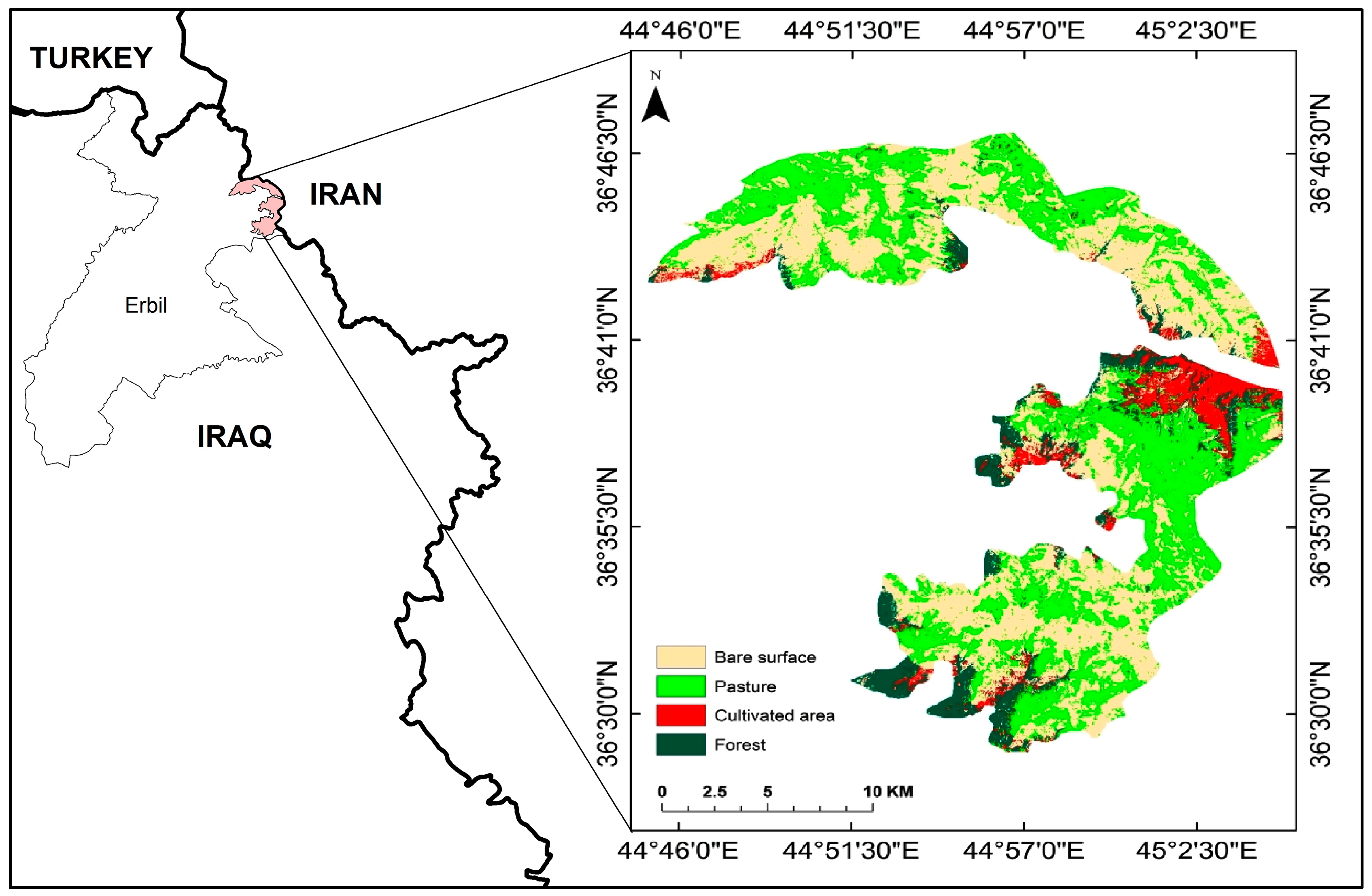
2.1. Study Area

HSCZ is located northeast of Erbil, Iraq [18], in the Zagros Mountain Range which shares a border with Iran Figure 1. The climate of the Choman district is hot and dry in summer, and cold and wet in winter, according to Mami-Khalan monthly weather station [19]. HSCZ covers the highest peak of mountains in Iraq, 3609 m above sea level. Geologically, the study area is covered by various types of bedrocks, which are made up of different types of igneous, metamorphic, and sedimentary rocks. The rock outcrops for the study site are mainly dominated by two types of rock units, which are the Walash Volcanic rock group and the Qandil Metamorphic series group; therefore, the study area is mostly rock-dominated, followed by pasture land [20].
The study area was totally evacuated and used as military bases in the 1980s. Three significant socio-economic events can be identified in the study area in the last three decades: (i) the displacement during 1980–1991 when all inhabitants of the region left their homes to flee armed conflict and most of the villages were devastated [21]; (ii) re-settlement by villagers moving back to their homesteads after uprisings and the First Gulf War in 1991 [22]; and (iii) urbanisation after the fall of Baghdad in 2003 [23].

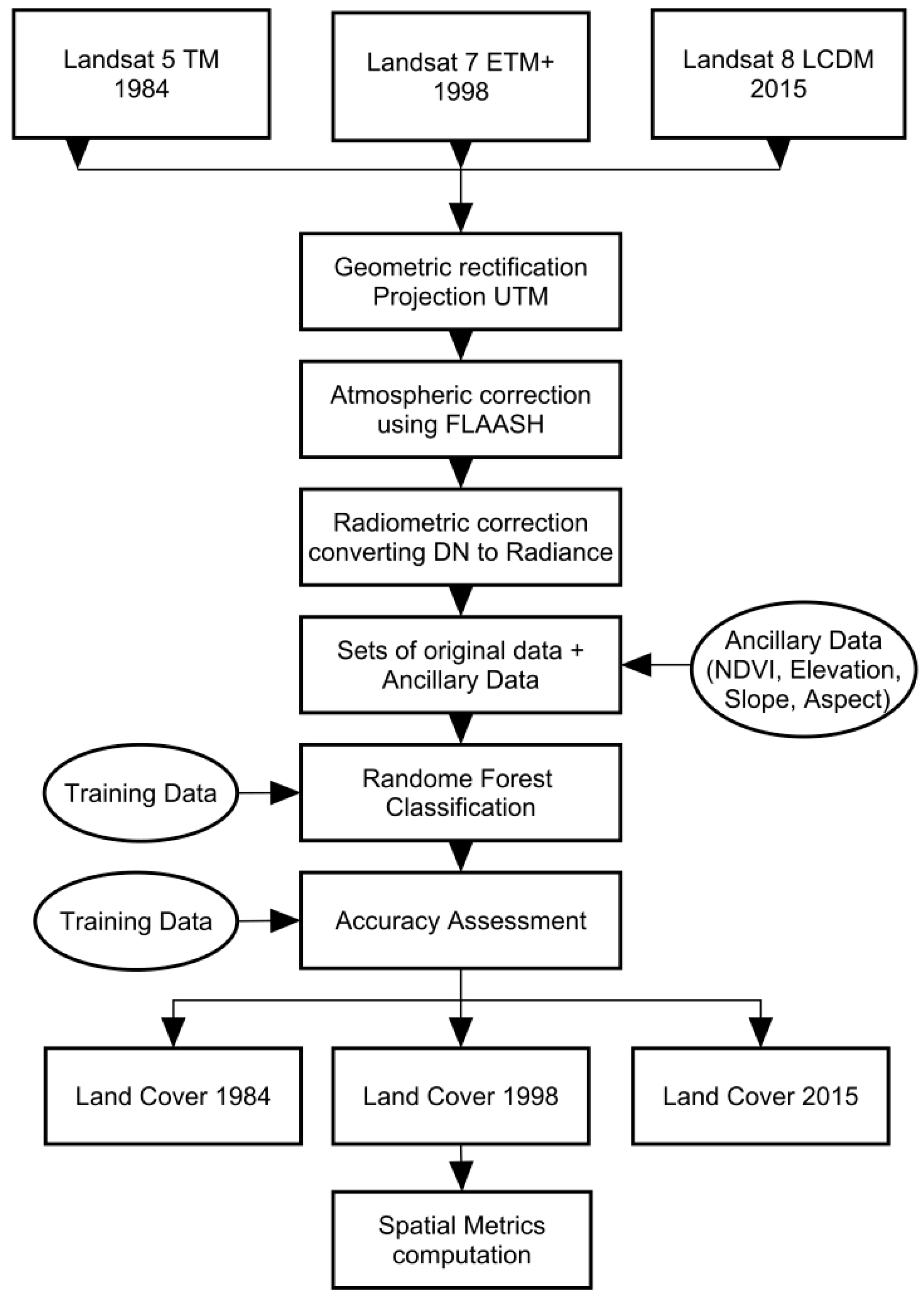
2.2. Satellite Imagery and Data Processing

Three satellite images of Landsat 5 Thematic Mapper (TM) for 1984, Landsat 7 Enhanced Thematic Mapper (ETM+) for 1998, and Landsat 8 Landsat Data Continuity Mission (LDCM) for 2015 with a spatial resolution of 30 m were used to map land cover (Table 1). Landsat 5 for 1984 was used in the 1980s during the Iraq-Iran war, when any socio-economic activities ceased in the region, and farmlands and cultivated lands were abandoned after Iran started opening fronts in Iraqi Kurdistan and it became a battlefield [22]. For the second period, a satellite image from 1998 was selected, as this period illustrates the human activity after the First Gulf War and saw an increase in rural residents [24]. The third period represents the time after the fall of Baghdad, which witnessed improvements of socio-economic conditions and the complete defeat of the Iraqi army in April 2003 [25], as can be seen in the Landsat 8 image for 2015.
The vegetation phenology of the region as a part of Zagros Mountains is most covered by mountain meadows with multitude of wild flora and fauna [26].
The different images in ENVI 5.3 (Environmental for Visualizing Images) software were all projected into Universal Transverse Mercator (UTM) Zone 38N, and then assembled in a raster Geographical Information System (GIS). Normalised Difference Vegetation Index (NDVI) was calculated as:
NDVI = (NIR − RED)/(NIR + RED)
from the NIR and RED bands.
Landsat images were processed and subset to include the entire area of the HSCZ [10]. As previously mentioned HSCZ is mostly rock and pasture-dominated lands by more than 85% therefore; images from 1998 and 2015 were categorised into four land cover classes; namely, bare surface, pasture, cultivated area, and forest. The 1984 image, it was categorised into three classes; specifically, bare surface, pasture, and forest, based on the expert knowledge as the cultivated lands during the war in the 1980s were abandoned. Expert knowledge in Choman district stated that most of the cultivated areas and agriculture activities are determined by agricultural. They usually select the cultivated areas around and near the villages or roads. Location of arable lands in the HSCZ is limited because the study area is covered by fewer villages.
Training sites were selected using high-resolution imagery from Google Earth, ESRI Arc Map base maps, and expert knowledge of the study gained from the Agricultural Department of Choman. We categorised the image by selecting representative samples for each land cover class ‘‘training sites” to extract pixel values from training polygons, generating signature files to identify the land cover classes in the entire digital image, and classifying land cover types present in a scene. To have variation within a class we collected 100 training polygon for each class throughout the image. Excessive training sites in the study area led to misclassification, the reason being that forest and cultivated area classes were rare classes of the area of interest. Therefore, we selected these rare classes only in areas where the rare classes were known to be found [27,28].
The classification was implemented using the random forest package [29] in R with all spectral bands, elevation, slope, aspect and ndvi band input data and training data for each class. Random forest classification produced a very accurate classification. Random forest is a non-parametric algorithm applicable to satellite image classification and regression. A random forest is generated from a collection of decision tree classifiers and provides more stable results than other methods [30,31]. An overview of the methodology is given in Figure 2.
Relief and shadow in rugged areas may lead to misclassification; therefore, using aspect and slope from the digital elevation data of the Shuttle Radar Topography Mission (SRTM) [32] as ancillary data during classification may improve the accuracy of the map by reducing the effect of relief [33,34].
The normalised difference vegetation index (NDVI) was also added into the raster stack. NDVI identifies vegetation and provides a measure of its health and validity; thus, there is a robust relationship between the NDVI and functional characteristics of vegetation [35]. We used NDVI as an additional raster dataset to study the impact on the classification accuracy [36].
Ancillary data are non-spectral information that are useful in characterising the classes for the area of interest [37]. Natya and Reyna [38] found that the classification based on training samples from various sources of ancillary data are more proper than classification based on pixel data. Integrating ancillary data into image classification increases the accuracy and discrimination for land use/land cover mapping [31]. For this study we used slope, aspect, elevation, and NDVI as ancillary data. SRTM data are distributed in tight file format (tif), which is raster format, although the elevation values are stored directly in each pixel of the raster grid that contains an integer value and represents the elevation of the grid cell [39].

2.3. Land Use Change and Accuracy Assessment

Franklin and Wulder [40] discussed the use of multi-temporal remote sensing images in support of identification of a variety of long-term land cover mapping in any large area. Lu et al. [33] stated the challenges that affect the classification accuracy of remote sensing imagery. Many errors appearing from the results of the classification can lead to missing the goal in terms of accuracy [41]. The accuracy of the classification increases by using multi-temporal imagery [42].
An error matrix resulting from classifying training set pixels assessed for images 1984, 1998, and 2015. Four measurements were used in the accuracy assessment process namely; user’s accuracy, producer’s accuracy, kappa’s coefficient, and overall accuracy. Computing correctly-classified pixels and dividing by the total number of pixels (the row total) generates the user’s accuracy, while correctly-classified pixels on a major diagonal divided by the number of training set pixels computes the producer’s accuracy. Overall accuracy is computed by dividing the total number of correctly classified pixels by the sum of the number of reference pixels [27].

2.4. Socioeconomic Changes

Generally, socioeconomic changes govern land resources in and around the protected area. It also determines current and future land use [8]. The area of interest has experienced a dramatic economic development in the past decade. The population has increased in the last six years by 1.14% from 2010 to 2015 [43]. Certainly, population growth is increasing in demand for resources and space. This rapid development, infrastructural facilities, and natural-cultural forces [44] affect socioeconomic development, the ecosystem, and environment. Landscape alterations are affected by demographic activities [45].

2.5. Quantifying Landscape Pattern

In order to characterise the changes of the HSCZ, a set of landscape metrics were selected. Landscape composition and configuration were used for quantifying landscape patterns and assessing land cover changes [46]. Based on a review of the recent literature regarding the use of landscape metrics for assessing landscape structure changes, the analysis was carried out at the class and landscape level. Eight metrics were selected at the class level and five metrics at the landscape level.
In terms of the landscape level, patch metric, area metric, shape metric, interspersion/juxtaposition and contagion metrics, and diversity metrics were used. Shape Index Mean (SHAPE_MN) quantifies the geometric complexity of the shape at several landscape levels [9,47]. Shape Index Area Weighted Index (SHAPE_AM) equals 1 if all patches are square and increases with complexity [47]. Higher values of SHAPE_AM indicate larger patches and, implicitly, more core area.
An assessment of landscape composition and configuration is performed at the class and landscape levels using FRAGTATS 4.2 for each individual image classification [47]. Table 2 represents different metrics of the landscape mosaic including composition, patch density, patch size, shape, landscape grain size, and patch adjacencies. Eight metrics were computed to quantify landscape structures. Metric selection was based on the objectives of the analysis for the three time points.
Metrics and indices for categorical maps are computed for analysing the landscape composition and configuration [46,47]. Spatio-temporal analysis in landscape patterns at various scales support ecological processes. Measuring the landscape patterns gives a better insight for understanding the relationship between landscape structure and the ecological process [48]. FRAGSTATS software package creates four output files corresponding to three levels in a table in text files of metrics namely; patch, class, and land [49].

3. Results

3.1. Accuracy Assessment

Table 3 shows the accuracy assessment with overall accuracy, producer’s accuracy, user’s accuracy, and Kappa coefficient [27,51] for the classified maps for 1984, 1998, and 2015. The accuracy assessments of the random forest classifications indicated overall accuracies of 96%, 97%, and 97% for the years 1984, 1998, and 2015, respectively. The Kappa coefficients of those dates were 0.94, 0.96, and 0.96, respectively. The most important variable of Landsat bands in the RF model that came out of predictors were band 5 (NIR, 0.85–0.88 nm), band 4 (Red, 640–670 nm), and band 3 (Green, 0.53–0.59), while DEM ranked the top four [52].

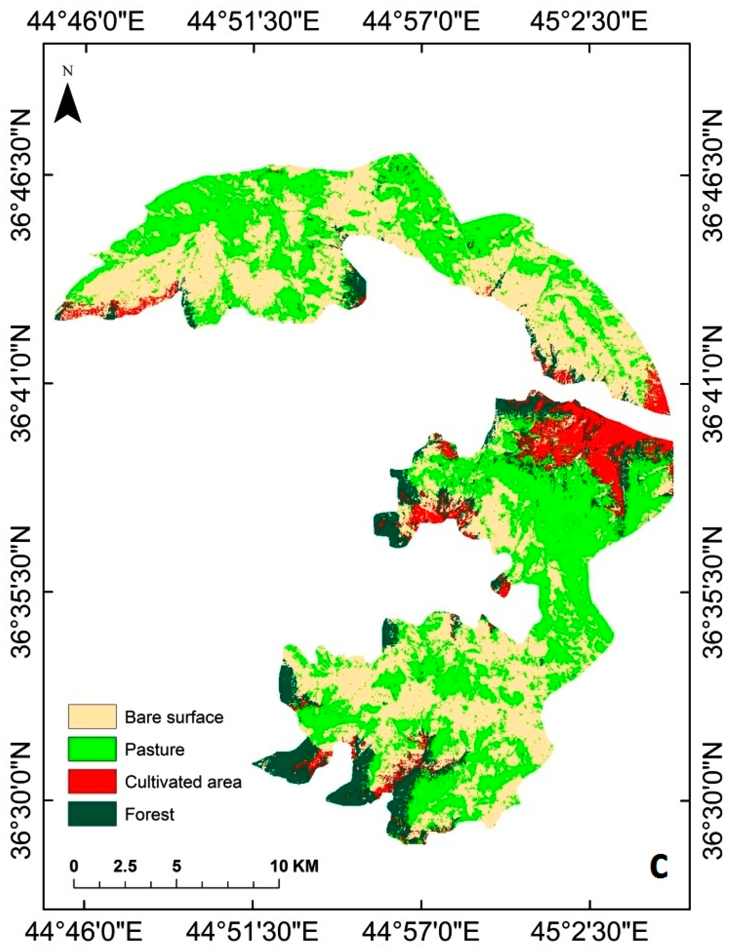
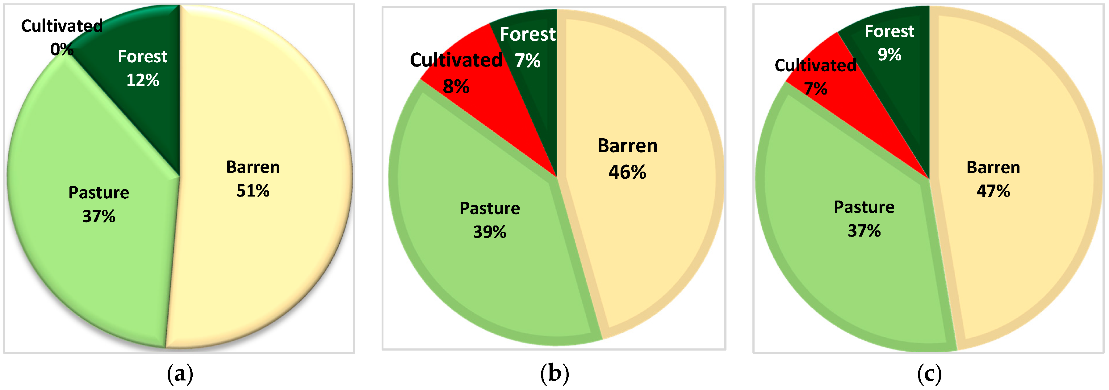
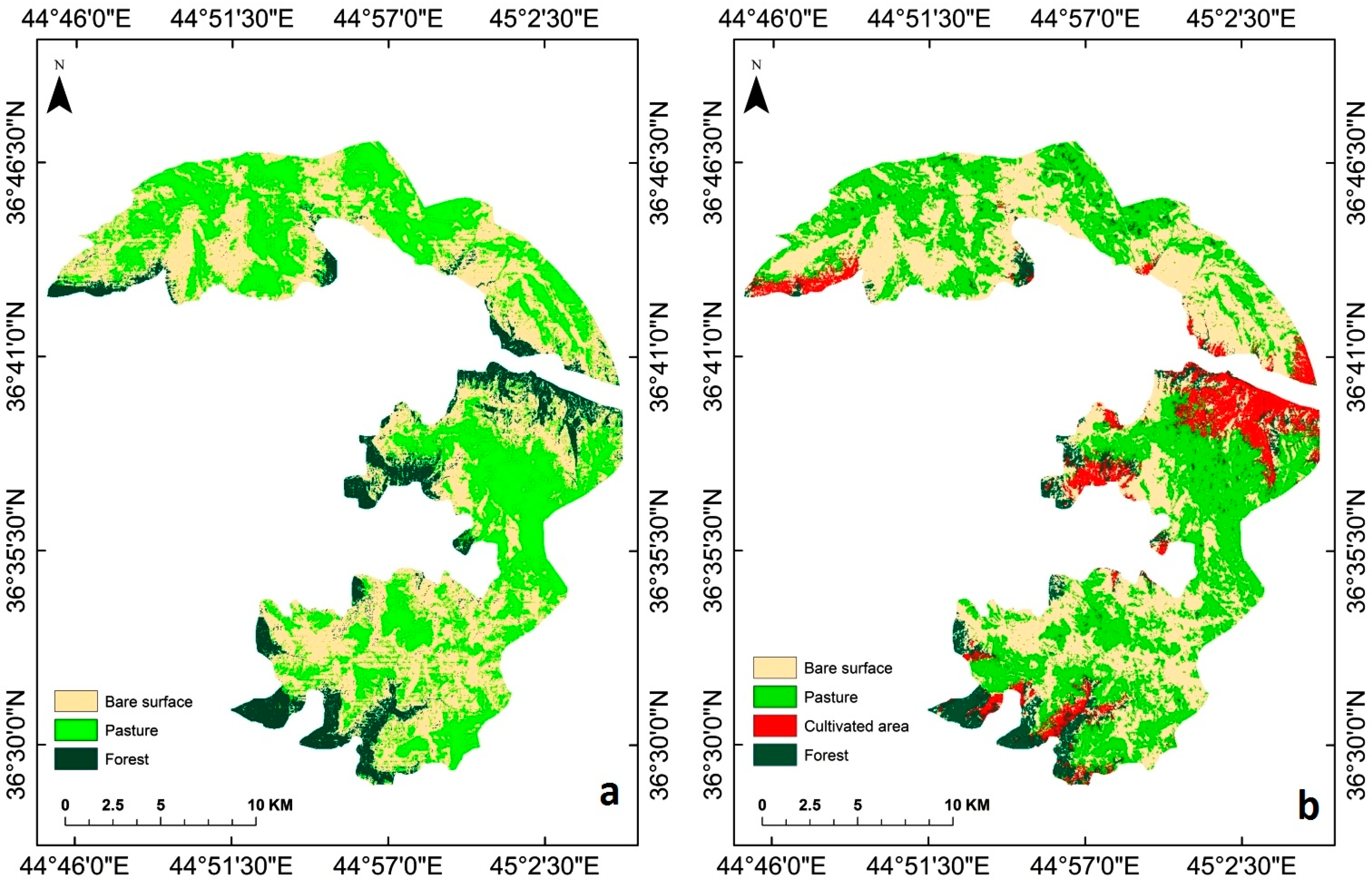
3.2. Landscape Structure and Dynamics

The [LULC] maps are shown in Figure 3 for three points in time (a, b, and c) and the classification area statistics in Table 4. The classified areas were measured in hectares and the percentage of land (PLAND) (Figure 4). Bare surfaces were the predominant landscape matrix in the study area respectively, for 1984, 1998, and 2015, which occupied 51.34%, 45.60%, and 47.38%, followed by pasture, which covered 37.07%, 39.35%, and 37.18%, respectively. Cultivated land covered 0%, 8.84%, and 6.57%, and forests covered 11.58%, 6.55%, and 8.86%, in the HSCZ for each year.
Changes are mapped for all land cover classes for all three points in time. The cultivated area was absent in 1984 [1] and it had greatly increased in 1998, by 8.48% as a result of socio-economic rural development promoted by the local government [43]. Between the years 1998 and 2015, the cultivated and pasture classes declined, while forest and bare surface increased.

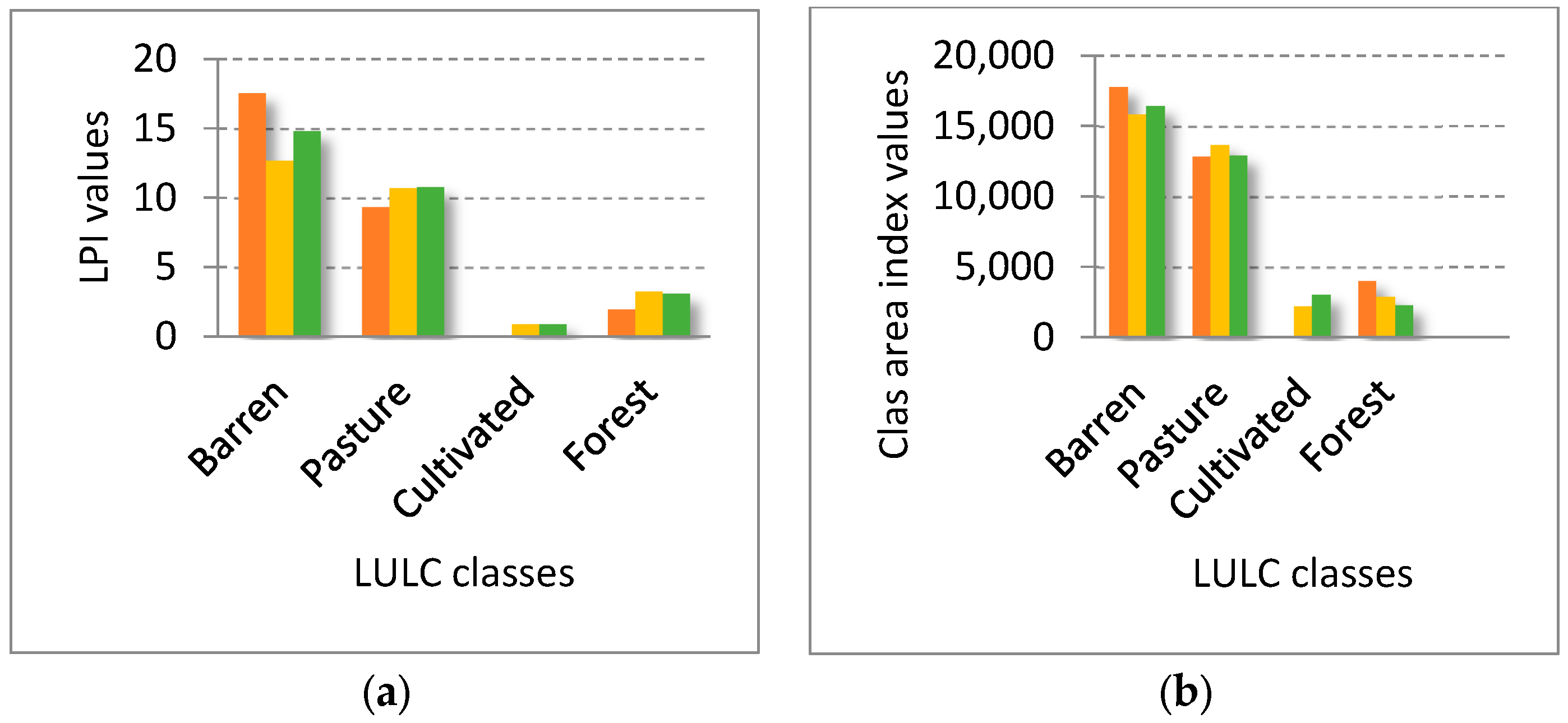
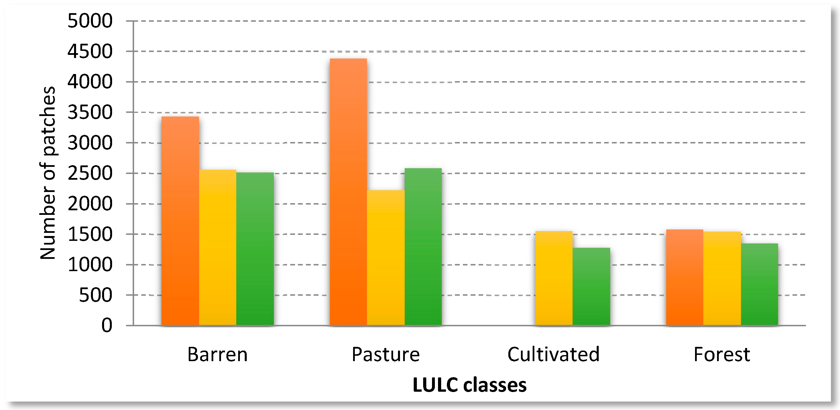
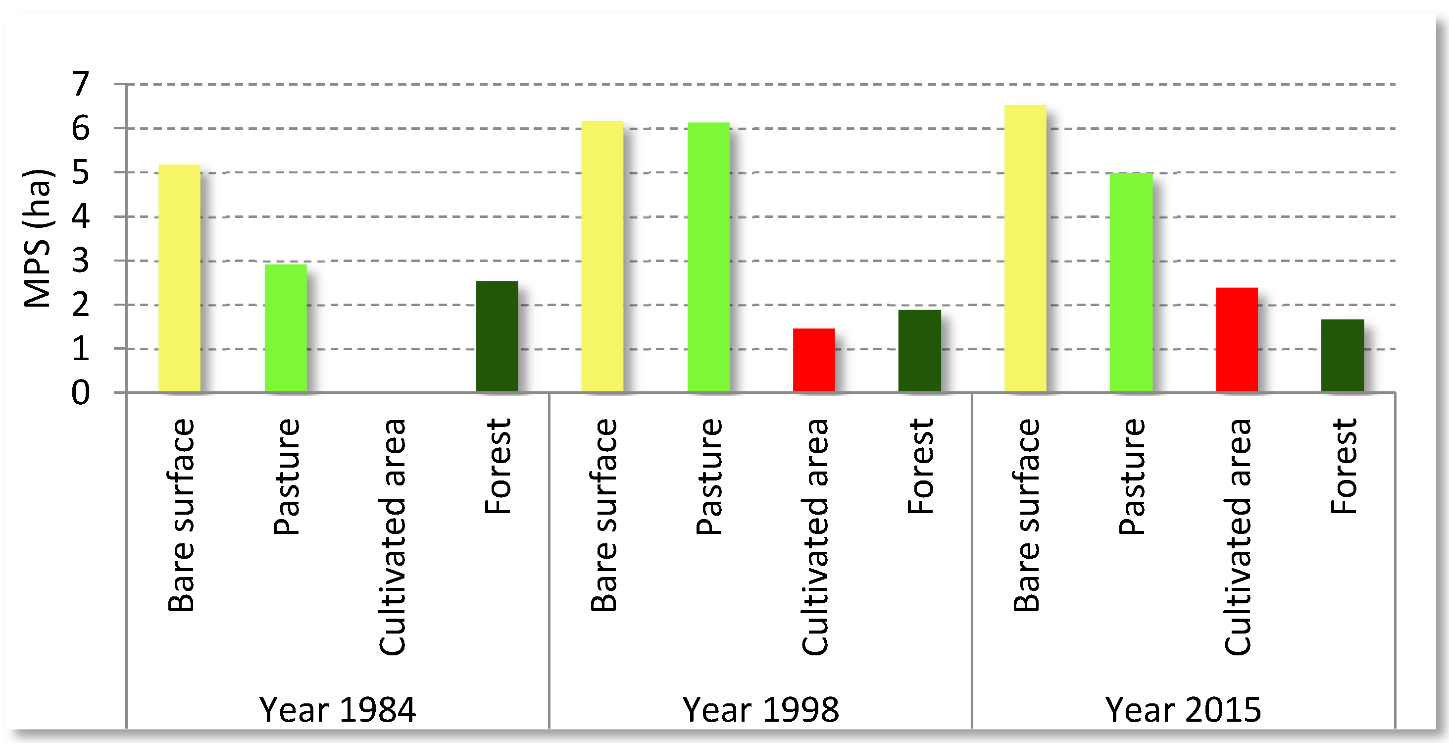
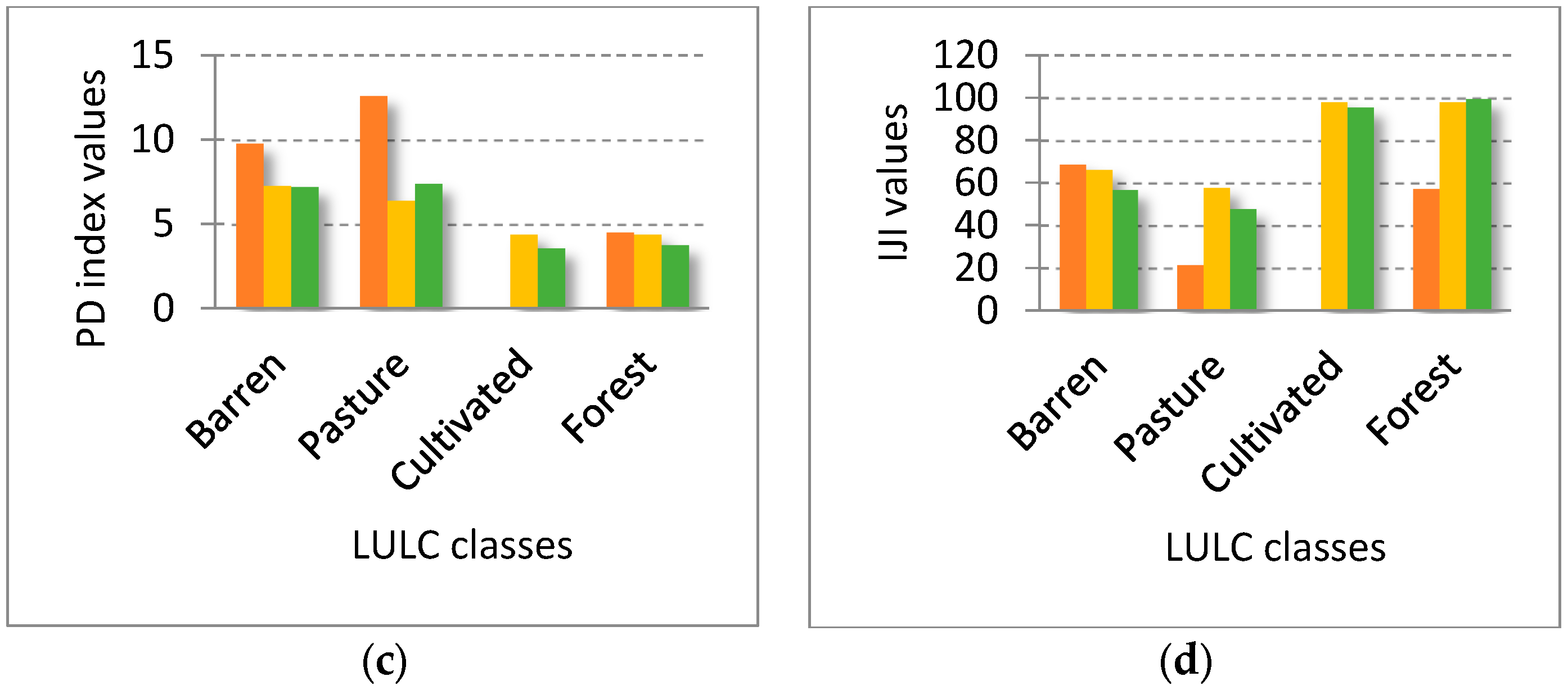
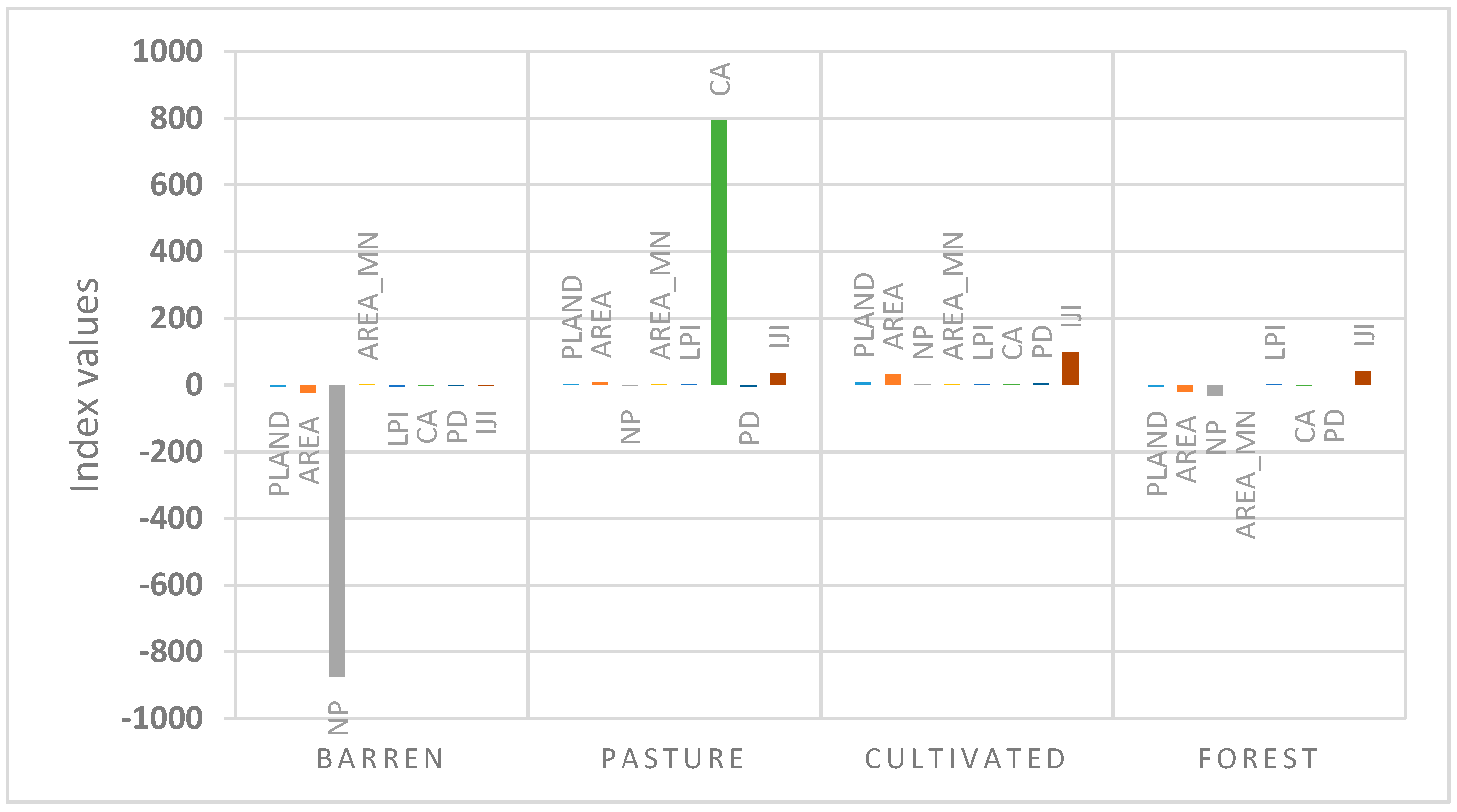
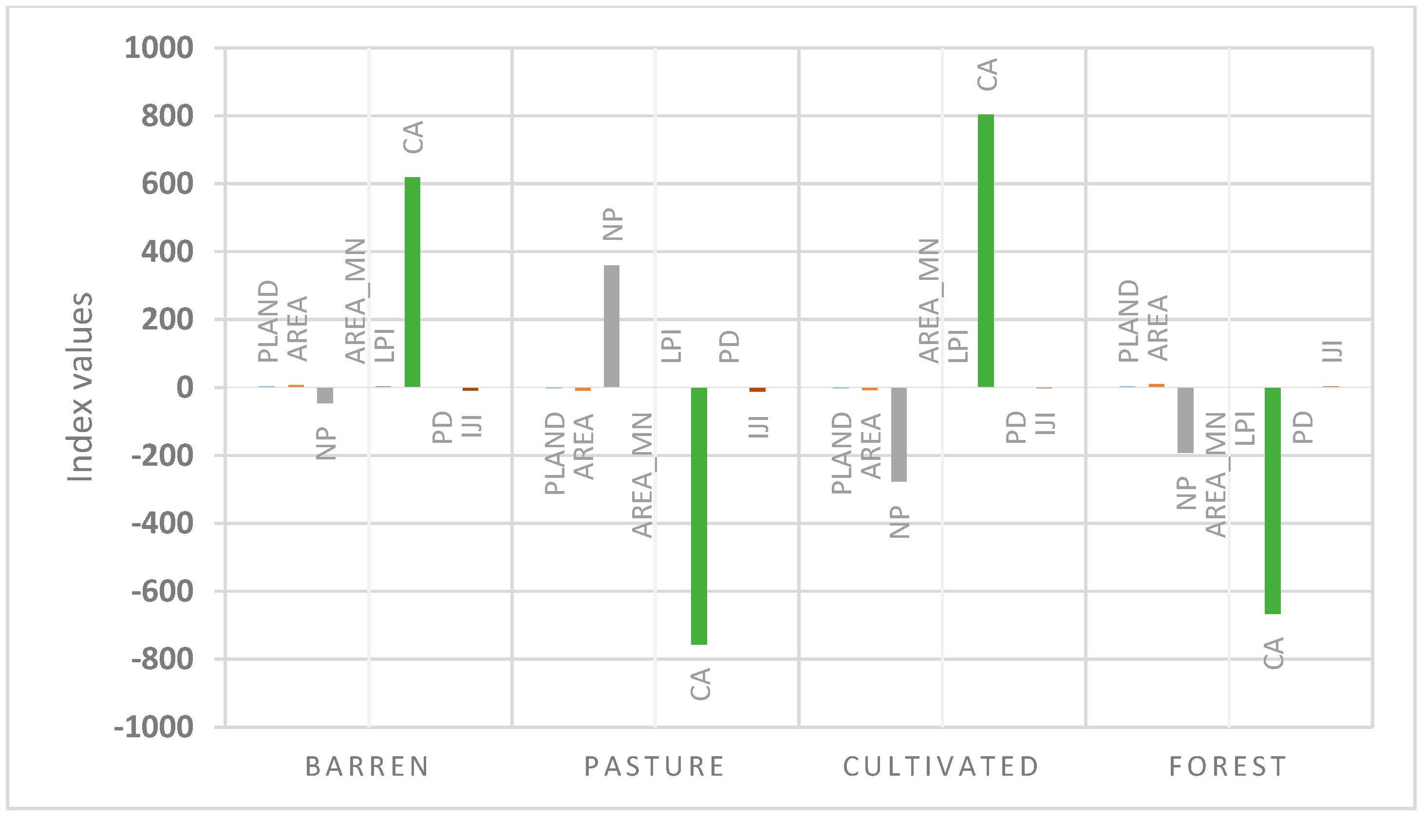
3.3. Analysis of Landscape Metrics at Class Level

Table 4 illustrates the evolution of the selected metrics for the years 1984, 1998, and 2015 for the HSCZ at the class level. Patch metrics and area metrics were used in order to compute fragmentation statistics of the LULC types at the class level.
The Number of Patches (NP) decreased across all LULC classes, except cultivated area, which witnessed a significant increment in the period from 1984 to 1998. The highest value was observed for the pasture class, which decreased by 2165 patches from 1984 to 1998. In the period 1998–2015, a significant reduction of barren, cultivated, and forest land was observed, whereas pastures increased by 360 patches. The increasing NP indicates ecosystem degradation [53].
However, a decreasing NP means less fragmentation in the area of interest. There was a rapid expansion of areas for cultivated and pasture lands between 1984 and 1998, Figure 5. We conclude that the bare surface, pasture, and forest classes were not affected by fragmentation, with NP decreasing during the analysed period between year 1984 and 1998, meanwhile, there was a rapid expansion for cultivated areas in the same time.
The mean patch size (MPS), also called the mean patch area (AREA_MN), is the average size of patches from a specific class [47] at the class level. MPS of the areas covered by barren, pasture, and cultivated areas showed an increase, whereas forest area witnessed a small reduction of MPS by 0.65 in the period 1984–1998.
However, there is a slight decrease in MPS for forest area by 0.22 and pasture area by 1.14 in the period 1998–2015, as shown in Table 4 and Figure 6. This implies that forest and pasture areas were undergoing conversion and fragmentation into bare and cultivated areas, or they had become more fragmented and heterogeneous.
There is a slight increase of the Largest Patch Index (LPI) for pasture, cultivated areas and forest from 1984 to 1998, while a sharp decrease can be seen for barren land, (Figure 7a). A decreasing trend in LPI indicates larger patches becoming fragmented into smaller patches and patchiness in the landscape over the time period. During the period from 1998 to 2015 the LPI increased for barren and pasture land showing an expansion in barren and pasture patches. However, the LPI was stable for cultivated areas with a slight decrease for forest by 0.2 in the period. Increasing LPI for forest is a desired trend in most national parks [54].
In 1984, bare surface occupied 198,383 ha followed with pasture by 143,240 ha of the total area. In contrast, forest covered only 44,750 ha without any cultivated areas present in HSCZ. Class area (CA) of cultivated and pasture land increased sharply by 2279 ha and 795 ha, respectively (Figure 7b). At the same time, barren and forest lands decreased by 1995 ha and 1075 ha from 1984 to 1998. The CA of bare surface increased in the last 17 years, followed by a continuing increase in cultivated area, whereas the CA for pasture and forest decreased for the period 1998 and 2015.
Patch Density (PD) for pasture area witnessed a significant reduction from 12.6 patches per 100 ha in 1984 to 6.4 patches per 100 ha in 1998, which decreased by 6.2 patches per every 100 ha over the 14-year period. The decrease in PD suggests that human activities have been restricted in the studied period. PD for barren land decreased from 9.8 to 7.3 and to 7.2 for classified maps from 1984, 1998, and 2015, respectively (Figure 7c).
However, lower values of PD in a class suggest that this class was present in a less fragmented state. The PD of cultivated areas increased from being totally absent in 1984 to 4.4 by 1998. This increase reflects unrestricted human activities in the area of interest. PD decreased for all land use/land cover classes between the years 1998 and 2015, except the pasture class, which increased slightly by 1 patch per100 ha (Table 4).
The interspersion and juxtaposition values (IJI), indicated that most of the cultivated and forest classes reported almost the same level of interspersion in 1998, indicating their high interspersion (Figure 7d). These two classes are intercalated among the other classes, which form a mosaic, and each class has a common border with all others. The greater complexity is reflected in an increase in the interspersion and juxtaposition index, as presented in Table 4. Furthermore, a higher degree of aggregation, or clumpiness, indicates more adjacency of patches and grater landscape heterogeneity. Figure 8 and Figure 9 illustrate both positive and negative changes for land use/land cover pattern of the HSCZ in two different time periods, from 1984 to 1998 and from 1998 to 2015, respectively.

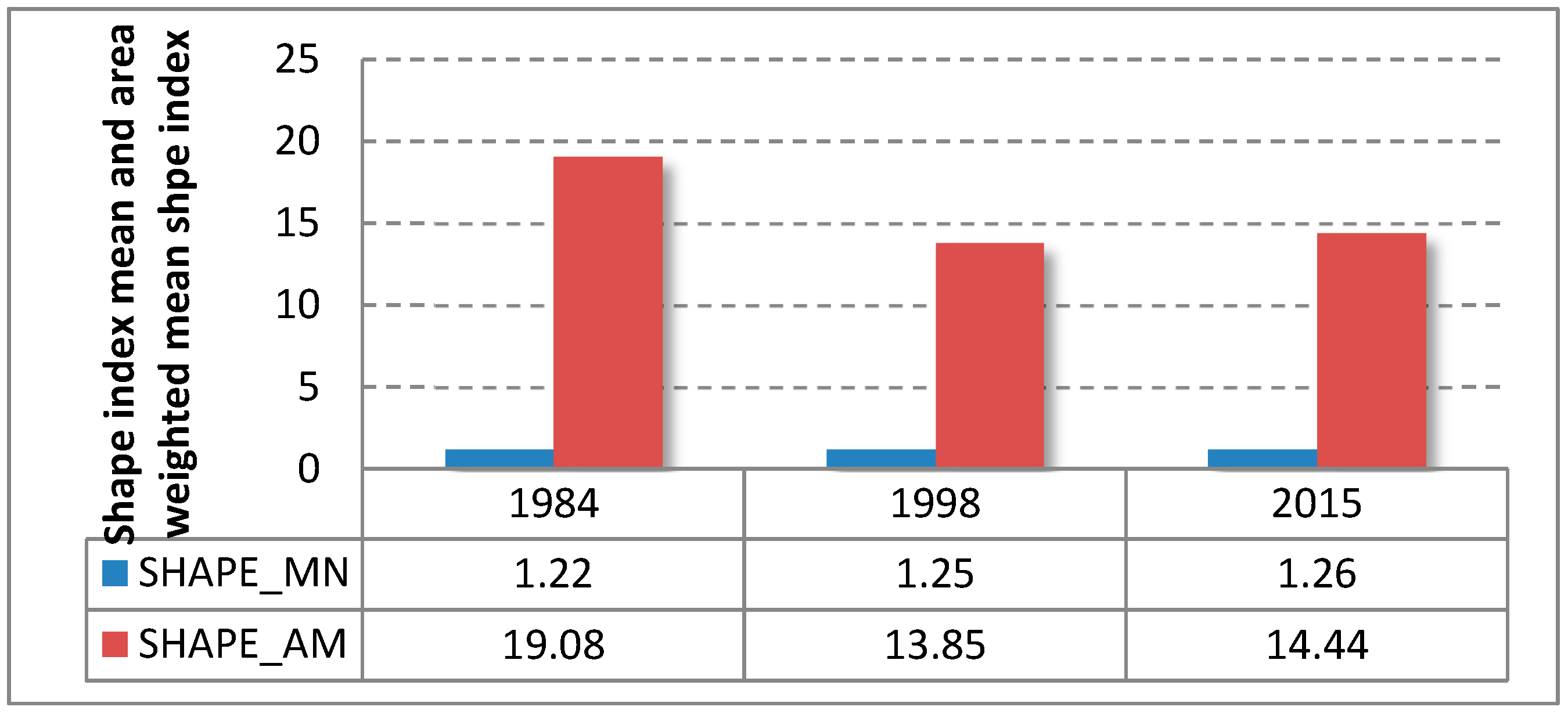
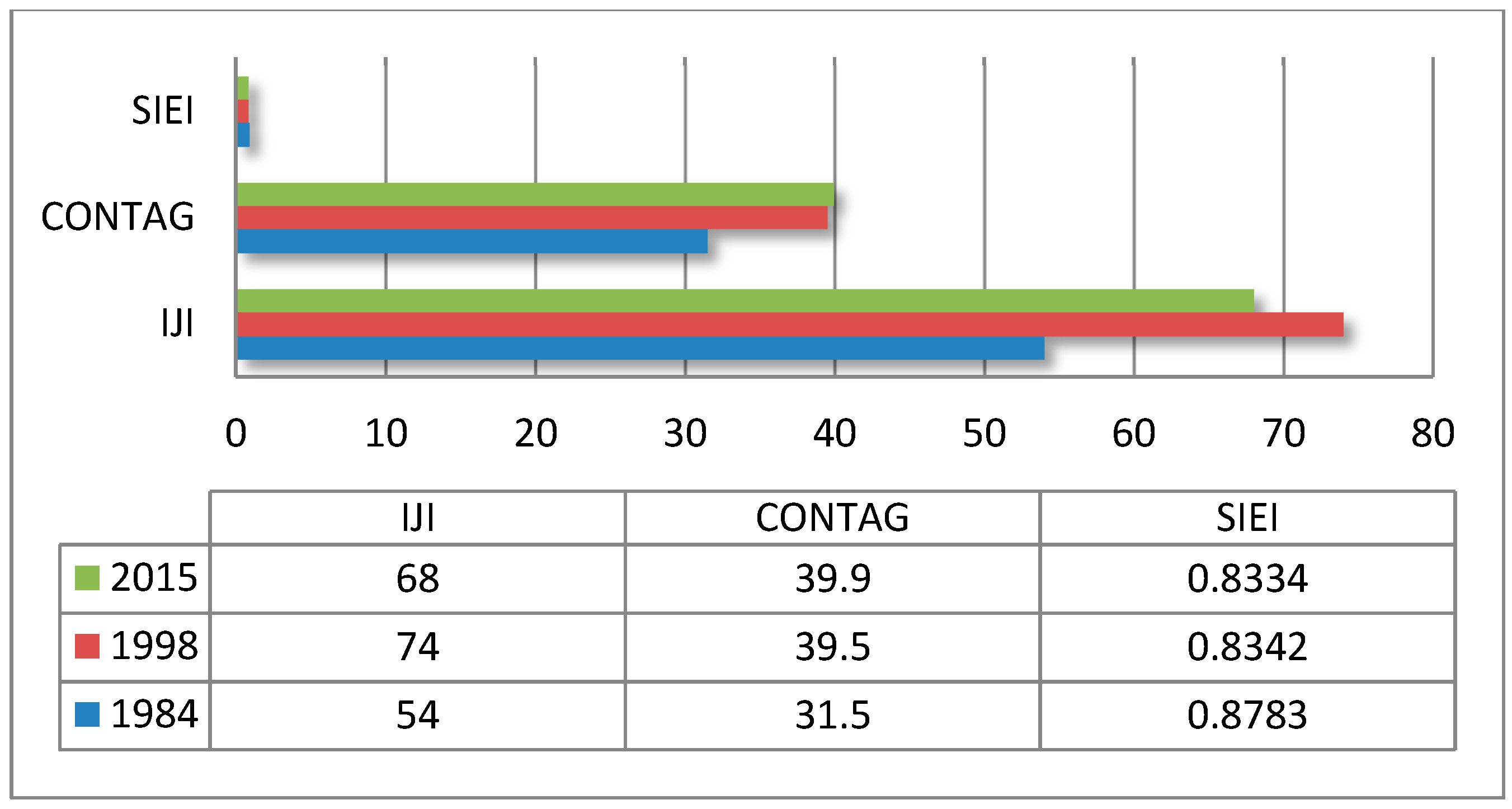
3.4. Analysis of Landscape Metrics at the Landscape Level

The value of SHAPE_MN varies between 1.22 and 1.26 from 1984–2015, indicating an almost regular outline (Figure 10). When the values of SHAPE_MN are similar, patches kept their form closer to a circular shape from 1998 to 2015. Over the studied period, patches have a slight tendency towards irregular shapes, specifying more core area and less edge.
In the HSCZ, SHAPE_AM in 1998 was the lowest (SHAPE_AM = 13.85), which means patches were smaller. The patches were larger for images from 1984 (SHAPE_AM = 19.08), followed by 2015 (SHAPE_AM = 14.44). The decrease of SHAPE_AM indicates less complexity of the landscape.
The interspersion and juxtaposition (IJI) values at the landscape level, increase from 54 in 1984 to 74 in1998. This increase in value indicates that the landscape is dominated by a few large (contiguous) patches. Meanwhile, the results of IJI display decreases from 74 in 1998 to 68 in 2015, which shows increasing subdivision and interspersion of patch types (Figure 11).
The results concerning the contagion index (CONTAG) indicate an increasing trend towards landscape aggregation, especially from 31.5 in 1984 to 39.5 in 1998, and almost in 2015 as well. This increase shows that the level of fragmentation is higher because of the existence of a number of privately cultivated areas. As mentioned earlier, this related to the migration of the villagers moving back to their homesteads and the return of farming to the area (Figure 11). In terms of Simpson’s Evenness Index (SIEI) high values of the SIEI indicate a high evenness in the distribution of areas among patch types. SIEI for all three images imply high evenness with 0.87, 0.83, and 0.83 for 1984, 1998, and 2015, respectively (Figure 11).
Overall, the land use/land cover LULC change analysis revealed that the most significant shifts were the reduction of bare surface and forest with an increase of cultivated and pasture areas between 1984 and 1998, whereas the process became reversed for the second period between 1998 and 2015, by decreasing cultivated and pasture surface areas and increasing in barren land and forest. Between 1984 and 1998, forest area decreased by 19,429 ha with a decrease of MPS, as well; thus, this reduction affects the wildlife corridors and habitat, negatively. Furthermore, the metrics concerning the landscape changes can tell us that the process of fragmentation isolate patches from each other. However, the fundamental idea behind any park in the world is to support the diversity of plants and animals through enhancing and protecting national park systems by reducing fragmented blocks. The increase of farmland is due to the continuing return of people to this region.

4. Discussion

In general, the major changes in the landscape for the study period occurred between 1984 and 1998, whereas the changes were smoothed between 1998 and 2015. The Landsat data revealed a clear shift in land cover dynamics after the 1980s, largely due to rapid growth of settlements [1,25] and demands for food and fuel.
Classification results show that the bare surface and pasture areas cover the largest parts of the study area, whereas forest and cultivated areas cover much smaller areas. As summarised in Table 4, bare surfaces covered 198,383 ha (51.34% of the land area) in 1984 and decreased to 176,209 ha (45.60%) in 1998. Between 1998 and 2015 bare surfaces increased again to 183,093 ha (47.38%). Cover by pastures increased by 8843 ha from 1984 to 1998. Thus, the decline in animal grazing that had taken place in the 1980s, because of the war, led to an expansion of pasture land from 143,240 ha in 1984 to 152,083 ha in 1998. However, after the fall of Baghdad and the rapid growth of settlements in the region, the pasture area declined from 152,083 ha in 1998 to 143,673 ha in 2015. Hence, this reduction of pasture land indicates increasing land use pressure for agriculture and animal grazing. The loss of soil fertility and desertification are two common concerns for decreasing the productivity of pasture plants as a result of exposing the plants to intensive grazing for extended periods of time. High animal stocking rate and grazing cattle consequently effects on soil quality and pasture production and composition, and prevents regrowth native ecosystems [55].
Results indicate that the total forest area decreased from 44,750 ha (11.58%) to 25,321 ha (6.55%) between 1984 and 1998. In the second period, 1998 to 2015, the forest area increased from 25,321 ha (6.55%) to 34,255 ha (8.86%). Human pressures on forests caused forest degradation in the first period which was due to an overexploitation of small trees from most accessible sites, which were used mainly as fuel for cooking and heating. Furthermore, demand for wood increased exponentially during the 1990s when there was a lack of electricity and fuel. Therefore, we conclude that population growth in the study area was also another reason that led to extensive forest degradation and deforestation. Increases in forest area from 1998 to 2015 indicate a better socio-economic state and better management practices. The results also reveal that cultivated areas grew sharply by 32,806 ha (8.48%) between 1984 and 1998, while, for the second period after the fall of Baghdad in 2003, the area of cultivated land decreased by 7408 ha (6.57%). The reason for this could be that, in the rural area, farm labour forces shift from agriculture into other activities as economic development proceeds. Socio-economic growth in the rural landscape has become a lasting concern [56]. The population of the study region declined dramatically from 1984–1991 [1]. In the 1990s and after the First Gulf War, abandonment of agricultural land was widespread in the study region [22].
Additionally, the expansion of human settlements and other infrastructure development activities, with the expansion of road networks after the First Gulf War and the fall of Baghdad in 2003, are major trends for increasing the cultivated area. Roads are also considered a major driver of forest fragmentation because they contribute to decreased patch connectivity and increased edge density [57]. The changes in cultivated land between 1984 and 1998 are the results of anthropogenic activities, which led to an increase of NP by 1559 patches. This increase of NP for cultivated areas is also confirmed by a decrease of MPS from 1.46 ha in 1984 to 0.94 ha in 1998, (Figure 5). At the same time decreasing PN for barren land, pasture and forest corresponds to decreases in area extent. Between 1998 and 2015 there is a decrease of NP and MPS of barren, cultivated, and forest land. An increase of NP indicates ecosystem degradation. We find that, over the past 31 years, human activities have caused fast and more extensive changes to the ecosystems.
An obligatory relocation of households out of the core zone took place in all districts and sub-districts in the 1980s. This research shows that the conversion of LULC classes can detect the influence of anthropogenic activities on the landscape and their effects on fragmentation, connectivity, and heterogeneity of the protected area. In general, more fragmented land in any national park leads to the decrease of movement for animals with less connectivity. The greater complexity and heterogeneity is reflected in an increase in the interspersion and juxtaposition index. The result of the interspersion and juxtaposition index shows a high heterogenic landscape for cultivated areas and forest, followed by pasture classes between 1998 and 2015 (Table 4).
Fragmentation and loss of forest land are considered the greatest threat to global biological diversity in national parks [58]. Fragmentation isolates the patches and negatively impacts species composition due to a reduction in forest area. Therefore, the fragmentation leads to more isolated patches. Finally, this research demonstrates the applicability of remote sensing and GIS analysis in using landscape pattern metrics.

5. Conclusions

A detailed land cover change analysis between each time period enabled a better understanding of changes in the HSCZ. The results showed that land use/land cover LULC in the study area is particularly dynamic and the structure of the landscape in the HSCZ has changed significantly during the 31-year study period. These changes are heterogeneous in space, time, and land cover distribution. The observed landscape changes are clearly linked to the agricultural sector, especially for the first period. Rapid landscape structure changes have been observed. There were drastic changes in the temporal and spatial patterns of the cultivated land cover class, which can have harmful impacts on the national park such as habitat loss, soil erosion, and land degradation.
Increases in the rural population and expansion of human settlements have caused irregular land use/land cover changes. Fuelwood was the most important energy source in the study region in the past decades and the improvement in forest cover was enabled by better socio-economic conditions and new restrictions on the collection of fuel and fire wood. As a result, the changes in the area of interest have slowed since 1998. The decreasing fragmentation is positive for biodiversity in the study area. In general, areas of bare surface and forest declined and became more fragmented for the years 1984 and 1998; at the same time, cultivated areas increased, with a continuing fragmentation of pasture land.
Remote sensing, GIS, and landscape metrics were used to prepare LULC maps, identifying, and analysing the changes that occurred over time. Understanding and monitoring of the dynamics of changes in land use/land cover is increasingly significant for the sustainable management of natural resources. Using landscape metrics provides many facilities in landscape ecology studies. Measuring the landscape serves as a useful tool to define the landscape structure in its various aspects, which includes the number of metrics; for instance, patch numbers and mean patch size are good indicators of the landscape pattern changes.

Acknowledgments

Financial support for this research was provided by Soran University. This work forms a part of a study and is supported by the Centre for Natural Resources Research (CNRR) Soran University and the Centre for Landscape and Climate Research (CLCR), University of Leicester, Department of Geography, University of Leicester. H. Balzter was supported by the Royal Society Wolfson Research Merit Award, 2011/R3 and the NERC National Centre for Earth Observation in the UK. The authors would like to thank Abdulwahid Gwany and the management of Halgurd Sakran National Park for their assistance and support in visiting the field. We also would like to thank Elvis Wang, editorial director at MDPI journal especially, and the three anonymous reviewers for their comments and suggestions on the manuscript.

Author Contributions

All authors contributed to the conception of the study. R.H. collected the input data, carried out, conceived, and designed the methodology, analysed the data, and wrote the paper; H.B. and K.K. supervised the research and contributed to the manuscript.

Conflicts of Interest

The authors declare no conflict of interest.

References

  1. Eklund, L.; Seaquist, J. Meteorological, agricultural and socioeconomic drought in the Duhok Governorate, Iraqi Kurdistan. Nat. Hazards 2015, 76, 421–441. [Google Scholar] [CrossRef]
  2. Ahmed, M.M. Emergence of Kurdistan Regional Government. In Iraqi Kurds and Nation-Building; Springer: New York, NY, USA, 2012; pp. 7–28. [Google Scholar]
  3. Švajda, J.; Fenichel, E.P. Evaluation of integrated protected area management in Slovakian National Parks. Pol. J. Environ. Stud. 2011, 20, 1053. [Google Scholar]
  4. Murray, G.; King, L. First Nations values in protected area governance: Tla-o-qui-aht tribal parks and Pacific Rim National Park Reserve. Hum. Ecol. 2012, 40, 385–395. [Google Scholar] [CrossRef]
  5. Krebs, C.J.; Boutin, S.; Boonstra, R. Ecosystem Dynamics of the Boreal Forest; New York7 The Kluane Project; Oxford University Press: Oxford, UK, 2001. [Google Scholar]
  6. Muller, F. Handbook of Ecosystem Theories and Management; CRC Press: Boca Raton, FL, USA, 2000. [Google Scholar]
  7. Ezebilo, E.E.; Mattsson, L. Socio-economic benefits of protected areas as perceived by local people around Cross River National Park, Nigeria. For. Policy Econ. 2010, 12, 189–193. [Google Scholar] [CrossRef]
  8. DeFries, R.; Hansen, A.; Turner, B.L.; Reid, R.; Liu, J. Land use change around protected areas: Management to balance human needs and ecological function. Ecol. Appl. 2007, 17, 1031–1038. [Google Scholar] [CrossRef] [PubMed]
  9. Forman, R.T. Land Mosaics: The Ecology of Landscapes and Regions (1995); Island Press: London, UK, 2014. [Google Scholar]
  10. Vorovencii, I. Quantifying landscape pattern and assessing the land cover changes in Piatra Craiului National Park and Bucegi Natural Park, Romania, using satellite imagery and landscape metrics. Environ. Monit. Assess. 2015, 187, 1–22. [Google Scholar] [CrossRef]
  11. Fahrig, L. Effects of habitat fragmentation on biodiversity. Annu. Rev. Ecol. Evol. Syst. 2003, 34, 487–515. [Google Scholar] [CrossRef]
  12. Henareh Khalyani, A.; Mayer, A.L.; Falkowski, M.J.; Muralidharan, D. Deforestation and landscape structure changes related to socioeconomic dynamics and climate change in Zagros forests. J. Land Use Sci. 2013, 8, 321–340. [Google Scholar] [CrossRef]
  13. Karami, A.; Sefidi, K.; Feghhi, J. Structure and spatial pattern of land uses patches in the Zagros Mountains region in the west of Iran. Biodivers. J. 2014, 15, 53–59. [Google Scholar] [CrossRef]
  14. Turner, M.G.; Gardner, R.H.; O’neill, R.V. Landscape Ecology in Theory and Practice; Springer: New York, NY, USA, 2001; Volume 401. [Google Scholar]
  15. Paliwal, A.; Mathur, V.B. Spatial pattern analysis for quantification of landscape structure of Tadoba-Andhari Tiger Reserve, Central India. J. For. Res. 2014, 25, 185–192. [Google Scholar] [CrossRef]
  16. Linh, N.; Erasmi, S.; Kappas, M. Quantifying land use/cover change and landscape fragmentation in Danang City, Vietnam: 1979–2009. ISPRS Int. Arch. Photogramm. Remote Sens. Spat. Inf. Sci. 2012, 1, 501–506. [Google Scholar] [CrossRef]
  17. Del Castillo, E.M.; García-Martin, A.; Aladrén, L.A.L.; de Luis, M. Evaluation of forest cover change using remote sensing techniques and landscape metrics in Moncayo Natural Park (Spain). Appl. Geogr. 2015, 62, 247–255. [Google Scholar] [CrossRef]
  18. Halgurd Sakran National Park. Available online: https://en.wikipedia.org/wiki/Halgurd_Sakran_National_Park (accessed on 25 January 2017).
  19. District of Choman. 2012. Available online: http://hawlergov.org/en/region.php?id=1330758915 (accessed on 25 January 2017).
  20. Sisakian, V.K. The Geology of Erbil and Mahabad Quadrangle; Iraq Geological Survey: Baghdad, Iraq, 1998. [Google Scholar]
  21. Brenneman, R.L. As Strong as the Mountains: A Kurdish Cultural Journey; Waveland Press: Long Grove, IL, USA, 2016. [Google Scholar]
  22. Lortz, M.G. Willing to Face Death: A History of Kurdish Military Forces—The Peshmerga—From the Ottoman Empire to Present-Day Iraq; Florida State University: Tallahassee, FL, USA, 2005. [Google Scholar]
  23. Eklund, L.; Persson, A.; Pilesjö, P. Cropland changes in times of conflict, reconstruction, and economic development in Iraqi Kurdistan. Ambio 2016, 45, 78–88. [Google Scholar] [CrossRef] [PubMed]
  24. McDowall, D. Modern History of the Kurds; IB Tauris: London, UK, 2003. [Google Scholar]
  25. Robinson, L. Masters of Chaos: The Secret History of the Special Forces; PublicAffairs: New York, NY, USA, 2005. [Google Scholar]
  26. Iraqi kurdistan. Available online: https://en.wikipedia.org/wiki/Iraqi_Kurdistan (accessed on 3 March 2017).
  27. Lillesand, T.; Kiefer, R.W.; Chipman, J. Remote Sensing and Image Interpretation; John Wiley & Sons: Hoboken, NJ, USA, 2014. [Google Scholar]
  28. Millard, K.; Richardson, M. On the importance of training data sample selection in random forest image classification: A case study in peatland ecosystem mapping. Remote Sens. 2015, 7, 8489–8515. [Google Scholar] [CrossRef]
  29. Liaw, A.; Wiener, M. Classification and regression by randomForest. R News 2002, 2, 18–22. [Google Scholar]
  30. Horning, N. Random Forests: An algorithm for image classification and generation of continuous fields data sets. In Proceedings of the International Conference on Geoinformatics for Spatial Infrastructure Development in Earth and Allied Sciences 2010, Hanoi, Vietnam, 9–11 December 2010.
  31. Breiman, L. Random forests. Mach. Learn. 2001, 45, 5–32. [Google Scholar] [CrossRef]
  32. Shuttle Radar Topography Mission (SRTM). Available online: https://www.jpl.nasa.gov/missions/shuttle-radar-topography-mission-srtm/ (accessed on 3 March 2017).
  33. Lu, D.; Hetrick, S.; Moran, E. Impervious surface mapping with Quickbird imagery. Int. J. Remote sens. 2011, 32, 2519–2533. [Google Scholar] [CrossRef]
  34. Eiumnoh, A.; Shrestha, R.P. Application of DEM data to Landsat image classification: Evaluation in a tropical wet-dry landscape of Thailand. Photogramm. Eng. Remote Sens. 2000, 66, 297–304. [Google Scholar]
  35. Baldi, G.; Guerschman, J.P.; Paruelo, J.M. Characterizing fragmentation in temperate South America grasslands. Agric. Ecosyst. Environ. 2006, 116, 197–208. [Google Scholar] [CrossRef]
  36. Raj, K.J.; SivaSathya, S. SVM and random forest classification of satellite image with NDVI as an additional attribute to the dataset. In Proceedings of the Third International Conference on Soft Computing for Problem Solving; Springer: New York, NY, USA, 2014. [Google Scholar]
  37. Varshney, P.K.; Arora, M.K. Advanced Image Processing Techniques for Remotely Sensed Hyperspectral Data; Springer Science & Business Media: Berlin, Germany, 2004. [Google Scholar]
  38. Natya, S.; Rehna, V. Land Cover Classification Schemes Using Remote Sensing Images: A Recent Survey. Br. J. Appl. Sci. Technol. 2016, 13, 1–11. [Google Scholar] [CrossRef]
  39. NASA Shuttle Radar Topography Mission (SRTM) Global 1 Arc Second Data. Available online: https://eros.usgs.gov/views-news/SRTM-30m-90m-data (accessed on 14 Apirl 2014).
  40. Franklin, S.; Wulder, M. Remote sensing methods in medium spatial resolution satellite data land cover classification of large areas. Prog. Phys. Geogr. 2002, 26, 173–205. [Google Scholar] [CrossRef]
  41. Foody, G.M. Status of land cover classification accuracy assessment. Remote Sens. Environ. 2002, 80, 185–201. [Google Scholar] [CrossRef]
  42. Rao, Y.; Zhu, X.; Chen, J.; Wang, J. An improved method for producing high spatial-resolution NDVI time series datasets with multi-temporal MODIS NDVI data and Landsat TM/ETM+ images. Remote Sens. 2015, 7, 7865–7891. [Google Scholar] [CrossRef]
  43. Ministry of Planning 2016. Kurdistan Regional Statistics Office-KRSO. Available online: http://www.mop.gov.krd (accessed on 25 January 2017).
  44. Gökyer, E. Understanding landscape structure using landscape metrics. In Advances in Landscape Architecture; InTech: Rijeka, Croatia, 2013. [Google Scholar]
  45. Kadioğullari, A.I.; Başkent, E.Z. Spatial and temporal dynamics of land use pattern in Eastern Turkey: A case study in Gümüşhane. Environ. Monit. Assess. 2008, 138, 289–303. [Google Scholar] [CrossRef] [PubMed]
  46. McGarigal, K.; Marks, B.J. FRAGSTATS: Spatial Pattern Analysis Program for Quantifying Landscape Structure; U.S. Department of Agriculture, Forest Service, Pacific Northwest Research Station: Portland, OR, USA, 1995.
  47. McGarigal, K.; Cushman, S.A.; Neel, M.C.; Ene, E. FRAGSTATS: Spatial Pattern Analysis Program for Categorical Maps; University of Massachusetts: Amherst, MA, USA, 2002. [Google Scholar]
  48. Turner, M.G. Spatial and temporal analysis of landscape patterns. Landsc. Ecolo. 1990, 4, 21–30. [Google Scholar] [CrossRef]
  49. FRAGSTATS Software Package. 23 January 2015. Available online: http://www.umass.edu/landeco/research/Fragstats/documents/fragstats.help.4.2.pdf (accessed on 25 January 2017).
  50. O’neill, R.; Hunsaker, C.T.; Timmins, S.P.; Jackson, B.L.; Jones, K.B.; Riitters, K.H.; Wickham, J.D. Scale problems in reporting landscape pattern at the regional scale. Landsc. Ecol. 1996, 11, 169–180. [Google Scholar] [CrossRef]
  51. Anderson, J.R. A Land Use and Land Cover Classification System for Use with Remote Sensor Data; US Government Printing Office: Washington, DC, USA, 1976; vol. 964.
  52. Salas, E.A.L.; Boykin, K.G.; Valdez, R. Multispectral and texture feature application in image-object analysis of summer vegetation in Eastern Tajikistan Pamirs. Remote Sens. 2016, 8, 78. [Google Scholar] [CrossRef]
  53. Turner, M.G.; Gergel, S.E. Learning Landscape Ecology: A Practical Guide to Concepts and Techniques; Springer-Verlag: New York, NY, USA, 2002. [Google Scholar]
  54. Jaafari, S.; Shabani, A.A.; Danehkar, A.; Nazarisamani, A. Spatial Pattern Analysis for Monitoring of National Parks: Sorkhe Hesar National Park, Iran. Res. J. Environ. Sci. 2014, 8, 90. [Google Scholar] [CrossRef]
  55. Pulido, M.; Schnabel, S.; Lavado Contador, J.F.; Lozano-Parra, J.; González, F. The impact of heavy grazing on soil quality and pasture production in rangelands of SW Spain. Land Degrad. Dev. 2016. [Google Scholar] [CrossRef]
  56. De Noronha Vaz, E.; Vaz, M.T.d.; Nijkamp, P. An Exploratory Landscape Metrics Approach to Agricultural Changes: Applications of Spatial Economic Consequences for the Algarve, Portugal; Tinbergen Institute: Amsterdam, The Netherlands, 2013. [Google Scholar]
  57. Forman, R.T. Road Ecology: Science and Solutions; Island Press: Washington, DC, USA, 2003. [Google Scholar]
  58. Vannette, R.L.; Leopold, D.R.; Fukami, T. Forest area and connectivity influence root-associated fungal communities in a fragmented landscape. Ecology 2016, 97, 2374–2383. [Google Scholar] [CrossRef] [PubMed]
Figure 1. Location map of Halgurd Sakran Core Zone (HSCZ) in the Kurdistan Region of Iraq.
Land 06 00018 g001
Figure 2. Flowchart of the general methodology.
Land 06 00018 g002
Figure 3. Random Forest Classification for HSCZ for (a) 1984; (b) 1998; and (c) 2015.
Land 06 00018 g003aLand 06 00018 g003b
Figure 4. Percentage of land (PLAND) in the HSCZ for years (a) 1984; (b) 1998; and (c) 2015.
Land 06 00018 g004
Figure 5. Landscape metrics at class level for Number of patch (NP) in HSCZ for years 1984, 1998, and 2015.
Land 06 00018 g005
Figure 6. Mean patch size (MPS) for land use/land cover classes of the HSCZ at three different times.
Land 06 00018 g006
Figure 7. Landscape metrics at class level for HSCZ 1984, 19988, and 2015: (a) class area; (b) largest patch index and (c) patch density; and (d) interspersion and juxtaposition.
Land 06 00018 g007aLand 06 00018 g007b
Figure 8. Changes in land use/land cover from 1984 to 1998 for metrics PLAND, AREA, NP, AREA_MN, Largest Patch Index (LPI), class area (CA), Patch Density (PD), and interspersion and juxtaposition (IJI).
Land 06 00018 g008
Figure 9. Changes in land use/land cover from 1998 to 2015 for metrics PLAND, AREA, NP, AREA_MN, LPI, CA, PD, and IJI.
Land 06 00018 g009
Figure 10. SHAPE_MN and SHAPE_AM for land use and land cover (LULC) changes of the HSCZ 1984, 1998, and 2015.
Land 06 00018 g010
Figure 11. Interspersion and juxtaposition IJI, Contagion index (CONTAG), and Simpson’s evenness index (SIEI) for LULC changes of HSCZ 1984, 1998, and 2015 at landscape level.
Land 06 00018 g011
Table 1. Satellite (sub-scene) images used in this study to quantify landscape patterns and land cover changes.
Satellite SensorsPath/RowAcquisition DateResolutionBand Nos.
Landsat 5 TM169/03518 August 198430 m1, 2, 3, 4, 5, 7
Landsat7 ETM+169/03513 September199830 m1, 2, 3, 4, 5, 7
Landsat 8 LDCM169/03524 August 201530 m1, 2, 3, 4, 5, 7, 8, 9
SRTM (1 arc)N36_E044/N36_E045September 201430 mGDEM
Table 2. Summary of landscape metrics used in this study (all formulas available in).
AcronymMetricDescriptionReference(s)
Class Level
PLANDPercentage of landscapeProportion of the landscape occupied by certain LULC classMcCarigal & Marks (1995) [46]
AREAAreaArea of patches (ha)McCarigal & Marks (1995) [46]
NPNumber of patchesNumber of patches in the landscape of the same LULC classMcCarigal & Marks (1995) [46]
LPILarge patch indexPercentage of the landscape comprised by the largest patch of the corresponding LULC classForman (1995) [9]
CAClass areaClass area (ha) Dominance indexMcCarigal & Marks (1995) [46]
PDPatch densityCalculation of the density of patches for each class within the landscapeMcCarigal & Marks (1995) [46]
AREA_MNMean patch size (MPS)Mean area of patches of the same LULC class (m2)McCarigal et al. (2002) [47]
IJIInterspersion and Juxtaposition indexMeasure of evenness of patch adjacencies, equals 100 for even, and approaches 0 for uneven adjacenciesMcCarigal & Marks (1995) [46]
Landscape Level
SHAPE_AMArea-weighted mean shape indexMeasures the complexity of patch shape of a particular class compared to a standard shape (square), by weighting patches according to their size. It equals 1 when all patches are square and increases with the complexity of patch shapesMcCarigal & Marks (1995) [46]
SHAPE_MNShape index meanComputes an area-adjusted measure (to a square) of the average shape complexity for each classMcCarigal & Marks (1995) [46]
IJIInterspersion/juxtaposition indexMeasure of evenness of patch adjacencies, equals 100 for even and approaches 0 for uneven adjacenciesMcCarigal & Marks (1995) [46]
CONTAGContag indexMeasure of configuration that degree of spatial aggregation of land cover typeO’Neill, Krummel et al. (1996) [50]
SIEISimpson’s evenness indexA measure of configuration that quantifies the distribution of area among patch typesSimpson (1949) [46]
Table 3. Land use/cover classification accuracies (%) for 1984, 1998, and 2015.
Land Use/Cover198419982015
P *U *PUPU
Bare surface969397989998
Pasture939797989897
Cultivated area0093968896
Forest879899969896
Overall accuracy969797
Overall Kappa Statistic0.940.960.96
Note: P * = Producers accuracy; U * = Users accuracy.
Table 4. Values of class land percentage, area, patch number, mean patch size, largest patch index, class area, patch density, and the interspersion and juxtaposition at the class level for the HSCZ in 1984, 1998, and 2015.
Land Use/Land Cover ClassMetricYearsChanges 1984–1998Changes 1998–2015
198419982015
BarrenPLAND51.3445.6047.38−5.741.78
AREA198,383176,209183,093−22.1746.884
NP343825632517−875−46
AREA_MN5.196.186.540.990.36
LPI17.612.714.8−4.91.9
CA17,85415,85916,478−1.995619
PD9.87.37.2−2.5−0.1
IJI69.0466.2156.72−2.83−9.49
PasturePLAND37.0739.3537.182.28−2.17
AREA143,240152,083143,6738.843−8.410
NP439122262586−2.165360
AREA_MN2.396.145.003.21−1.14
LPI9.410.710.81.30.1
CA12,89213,68712,930795−757
PD12.66.47.4−6.21
IJI21.6557.6348.0935.98−12.11
CultivatedPLAND08.486.578.48−1.91
AREA032,80625,39832.806−7.408
NP0155912821.559−277
AREA_MN01.462.401.460.94
LPI00.90.90.90
CA0227930832.279804
PD04.43.64.4−0.8
IJI098.0895.7498.08−2.34
ForestPLAND11.586.558.86−5.032.31
AREA44,75025,32134,255−19.4298.934
NP157915461354−33−192
AREA_MN2.551.901.68−0.65−0.22
LPI2.03.33.11.3−0.2
CA402729522286−1.075−666
PD4.54.43.8−0.1−0.6
IJI57.4398.1299.8140.691.69
Note: Negative values indicate loss and positive values indicate gain.

