Intra Prediction of Depth Picture with Plane Modeling

Abstract

In this paper, an intra prediction method is proposed for coding of depth pictures using plane modelling. Each pixel in the depth picture is related to the distance from a camera to an object surface, and pixels corresponding to a flat surface of an object form a relationship with the 2D plane surface. The plane surface can be represented by a simple equation in the 3D camera coordinate system in such a way that the coordinate system of depth pixels can be transformed to the camera coordinate system. This paper finds the parameters which define the plane surface closest to given depth pixels. The plane model is then used to predict the depth pixels on the plane surface. A depth prediction method is also devised for efficient intra prediction of depth pictures, using variable-size blocks. For prediction with variable-size blocks, the plane surface that occupies a large part of the picture can be predicted using a large block size. The simulation results of the proposed method show that the mean squared error is reduced by up to 96.6% for a block size of 4 × 4 pixels and reduced by up to 98% for a block size of 16 × 16, compared with the intra prediction modes of H.264/AVC and H.265/HEVC.

1. Introduction

Image processing using RGB-D video extends the conventional RGB video by using various information related to the distance of objects. Image processing using RGB-D video is actively studied in the fields of the face detection [1,2,3,4], object detection and tracking [5,6,7], SLAM (Simultaneous Localization and Mapping) [8,9], and so on. As application through the RGB-D videos increases, the need for depth video encoding will also be increased. The depth video encoding method can be categorized as point cloud encoding [10,11,12,13,14,15], mesh structure [16,17,18,19,20,21], and the conventional encoding method such as adopted by H.264/AVC [22,23,24,25,26,27,28]. The point cloud compression algorithms focus on the static scanned point cloud, and cannot handle the replicate geometry information contained in depth frames. In the mesh-based depth schemes, extracting the mesh from each raw depth frame costs additional computing and accordingly coding complexity increases. However, the depth pixel has a high dynamic range that is different from the 8-bit pixel in the traditional RGB picture. The coding schemes designed for 8-bit video component signal encoding may not be directly applicable to the depth picture compression.

Video can be efficiently compressed by reducing the spatial redundancy in a picture, which is that adjacent pixels in same object have similar pixel values. The spatial redundancy can be reduced by encoding the difference between the value predicted by the neighboring pixels and original value. The video encoding standards such as H.264/AVC and H.265/HEVC provide intra-picture prediction modes such as direction modes and DC mode for reducing the spatial redundancy. However, it is hard to apply conventional intra prediction methods for the color picture to the depth picture because the depth picture has different characteristics from the color picture such as distribution change of pixels according to surface type. Therefore, the intra prediction methods for the depth picture have been studied. Liu [29] introduced the new intra coding mode that is to reconstruct depth pixels with sparse representations of each depth block to intra prediction. Fu [22] proposed improvement of efficiency of the intra-picture encoding for filtering the noise by using error model of depth value. Lan [30] introduced the context-based spatial domain intra mode. For its intra prediction mode, only the neighboring already predicted pixels belonging to the same object can be used to make prediction. Shen [31] proposed the edge-aware intra prediction in H.264/AVC that predicts by determining a predictors based on edge locations in a macroblock. However, conventional methods of intra prediction for the depth picture are dependent on location information of objects in the picture.

In this paper, we propose the non-direction mode in the intra prediction for the depth picture. The conventional non-direction mode for the intra prediction such as the plane mode in H.264/AVC or the planar mode in H.265/HEVC predicts the macroblock through the linear function whose parameters are computed using reference samples. In contrast, the proposed intra-prediction mode assumes that the macroblock is composed of a plane surface. The plane surface in the macroblock is estimated by modeling the plane through the depth values. The proposed mode can be applied using the variable-size block. We compare the proposed mode with the conventional intra prediction modes and show that the proposed method is more efficient for depth picture than the conventional intra prediction methods.

2. Conventional Intra Prediction Methods

2.1. Intra Prediction in H.264/AVC

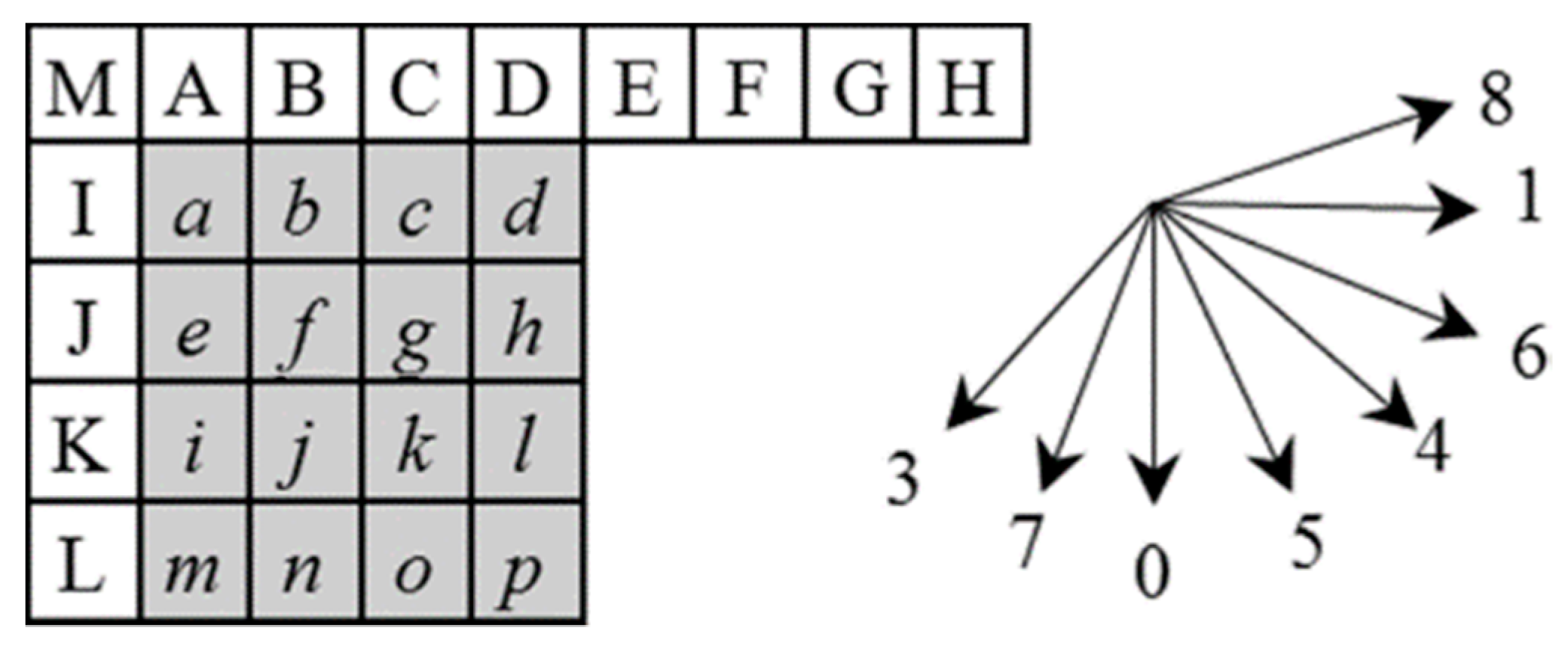
H.264/AVC uses the intra-picture prediction to reduce the high amount of bits encoded [32,33,34,35,36]. In the intra prediction, a macroblock is predicted based on adjacent previously intra- or inter-predicted blocks. H.264/AVC has 9 prediction modes for 4 × 4 and 8 × 8 luma blocks, 4 prediction modes for a 16 × 16 luma block, and 4 prediction modes for a chroma block. Figure 1 shows pixels (a, b, …, p) in a 4 × 4 luma block to be predicted from the adjacent previously predicted pixels (A, B, …, M) of the upper and left sides. The 9 prediction modes for a 4 × 4 luma block are as follows: 0-vertical, 1-horizontal, 2-DC, 3-diagonal down left, 4-diagonal down right, 5-vertical right, 6-horizontal down, 7-vertical left, and 8-horizontal up.

The 4 prediction modes for a 16 × 16 luma block are as follows: 0-vertical, 1-horizontal, 2-DC, and 3-plane. The vertical mode, the horizontal mode, and the DC mode are same as modes for the 4 × 4 luma block. The plane mode predicts pixels by a linear function. According to H.264/AVC specification [32], the linear function is as follows:

$$\tilde{P}[x,y]=(w_1+w_2\times (x-7)+w_3\times (y-7)+16)>>5,$$

(1)

where ‘>>’ means the bitwise right shift operator, [x, y] represents a position of the pixel in the macroblock, $w_1,w_2,w_3$ represent the intermediate parameters. The parameters are computed from the reference pixels:

$$\begin{array}{c}{w}_1=16\times (P[-1,15]+P[15,-1])\\ w_2=(5\times H+32)>>6\\ w_3=(5\times V+32)>>6\\ H={\sum }_{x^{\prime }=0}^7(x^{\prime }+1)\times (P[8+x^{\prime },-1]-P[6-x^{\prime },-1])\\ V={\sum }_{y^{\prime }=0}^7(y^{\prime }+1)\times (P[-1,8+y^{\prime }]-P[-1,6-y^{\prime }])\end{array},$$

(2)

where $P[x^{\prime },-1]$ and $P[-1,y^{\prime }]$ mean the reference pixels at top and left. In the parameters of the linear function, $w_1$ means the sum of the top-right reference pixel and the bottom-left reference pixel, $w_2$ means the average of the top reference pixels, and $w_3$ means the average of the left reference pixels. Thus, results of prediction through the plane mode are continuous and smooth, and this mode works well in smooth areas, while having known problem that the result of prediction can be discontinuous at the block boundary.

The intra prediction for the chroma elements is defined for three possible block sizes, an 8 × 8 chroma block in 4:2:0 format, an 8 × 16 chroma block in 4:2:2 format, and a 16 × 16 chroma block in 4:4:4 format. The prediction modes for these cases are the same as for the 16 × 16 luma block, but the order of these prediction modes is different as follows: 0-DC, 1-horizontal, 2-vertical, and 3-plane.

2.2. Intra Prediction in H.265/HEVC

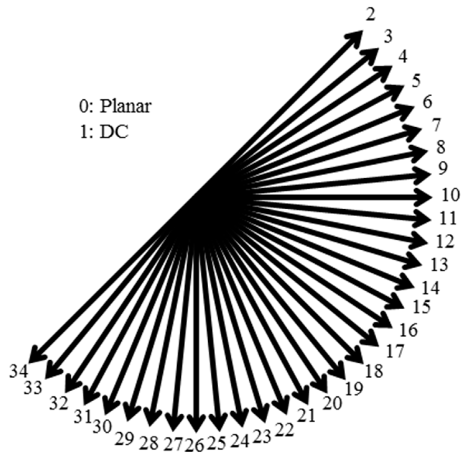
While the macroblock is the unit of intra prediction in H.264/AVC, a prediction block (PB) is the unit of the intra prediction in H.265/HEVC [37,38,39,40]. The size of PB is allowed to be 64 × 64, 32 × 32, 16×16, 8 × 8, and 4 × 4. The range of supported sizes for the prediction mode has been increased in H.265/HEVC. H.265/HEVC introduces a planar mode which guarantees continuity at block boundaries and is desirable. H.265/HEVC employs 35 different modes as shown in Figure 2, including 33 angular modes, the DC mode, and the planar mode to predict PB. H.265/HEVC can use the lower left and the above right if they are already prediction. Therefore, to predict the current PU of size M × M, a total of 4M + 1 spatially neighboring reference samples may be used.

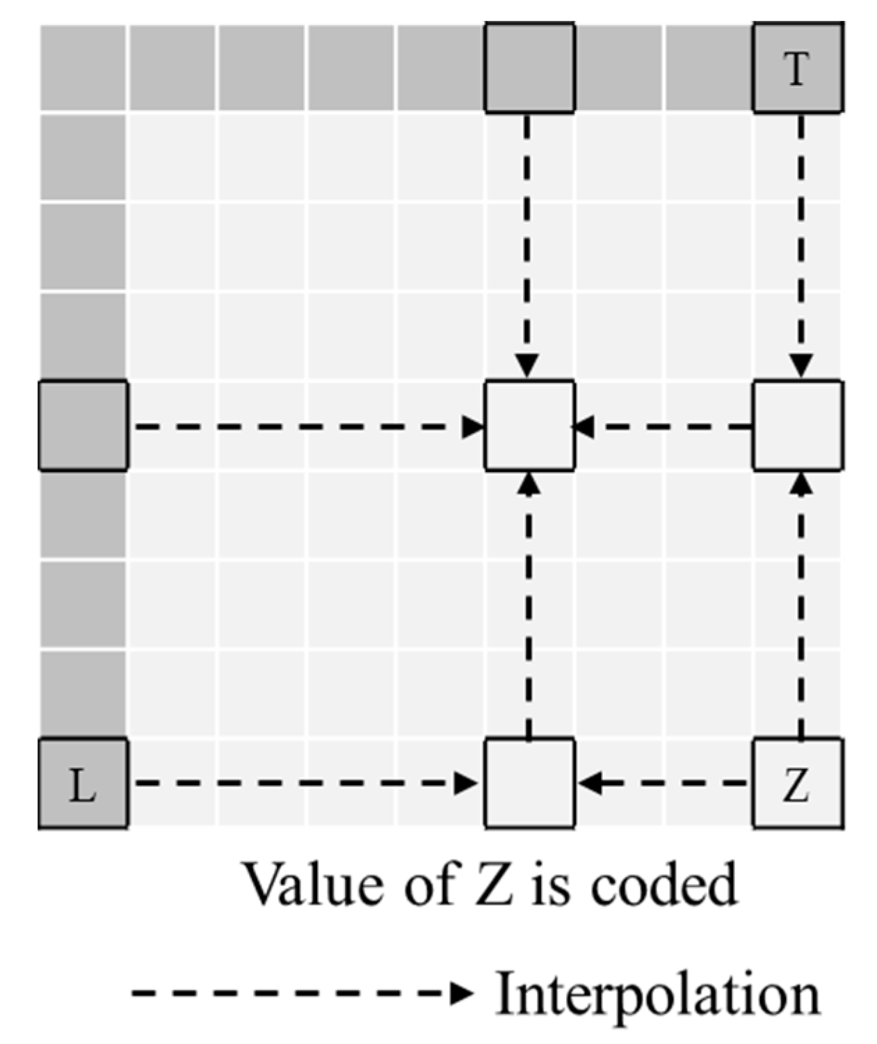
H.265/HEVC supports the planar mode as a non-directional prediction mode similar to the plane mode in H.264/AVC. The planar mode improves the discontinuity problem in the block boundary of the plane mode. In planar mode, the bottom-right sample is signalled in the bitstream, the rightmost and bottom samples are linearly interpolated, and the middle samples are bilinearly interpolated from the border samples [39]. Figure 3 shows the intra prediction through the planar mode.

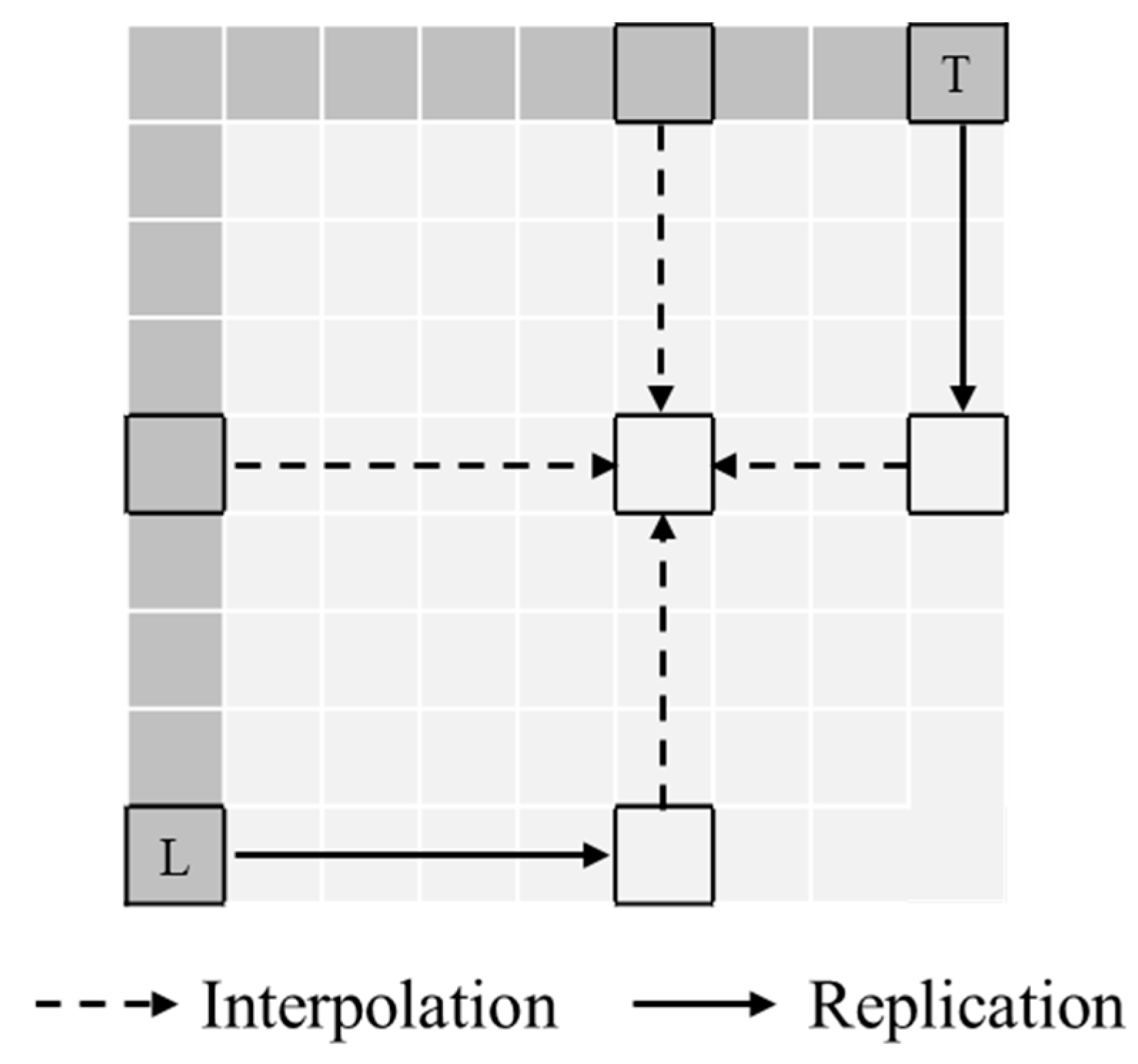
The planar mode should require not only the reference samples but also the bottom-right sample. The planar + DST mode is introduced to solve this problem [40]. In planar + DST mode, the bottom-right sample is estimated to the average of the reference samples of top-right and bottom-left. The computation of this prediction can be simplified. When Z = (L + T) >> 1, the bilinear interpolation can be replaced with the average of two linear interpolations (horizontal and vertical) as shown in Figure 4. The prediction computation is as follows:

$$\begin{array}{c}\tilde{P}[x,y]=(P_V[x,y]+P_H[x,y]+N)>>({\log }_{2}N+1)\\ P_V[x,y]=(N-y)\times R[x,0]+y\times R[0,N]\\ P_H[x,y]=(N-x)\times R[0,y]+x\times R[N,0]\end{array},$$

(3)

where x and y denote locations of the samples, N stands for total number of sample, R[x, y] stands for the reference sample of position (x, y).

The plane mode of H.264/AVC calculates a bilinear model using the reference samples to predict pixels. In contrast, the planar mode of H.265/HEVC predicts pixels by interpolating each pixel using a reference sample and a bottom-right sample (or reference samples of top-right or bottom-left). The planar mode keeps the benefits of the plane mode while preserving continuities along block boundaries.

3. Proposed Intra Prediction Method for Depth Picture

In this paper, an intra prediction mode by plane modeling is proposed. The proposed prediction mode predicts the pixels by planar surface, similar to the plane mode in H.264/AVC or the planar mode in H.265/HEVC. The prediction method by plane modeling can be applied to the variable-size blocks.

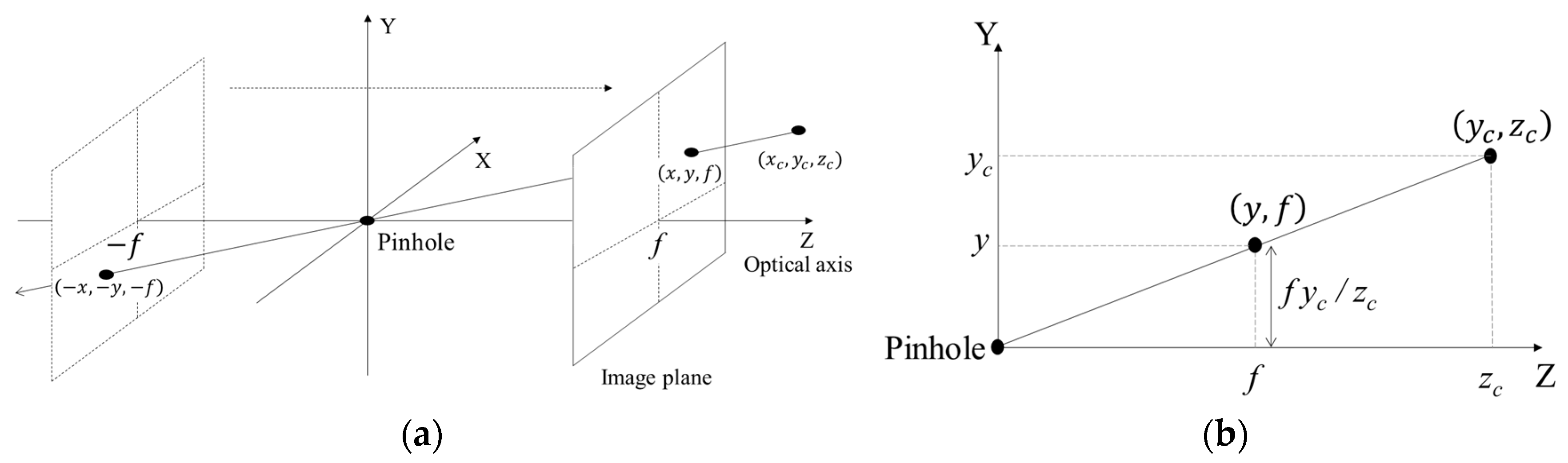
3.1. Pinhole Camera Model

The camera can be considered by a kind of device of coordinate transformation. A coordinate of the point in 3D space is transformed into the coordinate of 2D virtual plane by the camera. The pinhole camera model represents the relationship between coordinates of 3D space and 2D virtual plane. In the pinhole camera model, the camera optical axis is set to z-axis and the pinhole to the origin. A point in position (x_c, y_c, z_c) of 3D space is projected onto a point in position (−x, −y, −f), which is on the virtual plane, as shown in Figure 5a. f means a focal length that is the distance between the pinhole and the virtual plane. The phase of a projected image is reversed after passing the pinhole. To solve this problem, the virtual plane is moved to front the pinhole. Then, the point of 3D space is projected onto a point in position (x, y, f) of a moved virtual plane, which is defined as the image plane. The relationship between coordinates of 3D space and the image plane is calculated as follows:

$$\begin{array}{c}f:x=z_c:x_c\to x=f\frac{x_c}{z_c}\\ f:y=z_c:y_c\to y=f\frac{y_c}{z_c},\end{array}$$

(4)

3.2. Plane Modeling

A plane surface in the 3D space is represented as follows:

$$a_p{x}_c+b_p{y}_c+c_p=z_c,$$

(5)

where $a_p$, $b_p$, and $c_p$ are plane factors. The matrix equation is obtained by substituting $p_{c_i}(1\le i\le n)$ in a region into Equation (5) as follows:

$$\begin{array}{l}AR=B\hfill \\ A=\left[\begin{array}{ccc}{x}_{c_1}& y_{c_1}& 1\\ x_{c_2}& y_{c_2}& 1\\ & ⋮& \\ x_{c_n}& y_{c_n}& 1\end{array}\right] B=\left[\begin{array}{c}{z}_{c_1}\\ z_{c_2}\\ ⋮\\ z_{c_n}\end{array}\right] R=\left[\begin{array}{c}{a}_p\\ b_p\\ c_p\end{array}\right]\hfill \end{array},$$

(6)

where A is the matrix for the camera coordinates of x and y, B is the matrix for the camera coordinate of z, and R is the matrix for plane factors a_p, b_p, c_p. In (6), R can be obtained by calculating A⁻¹. However, A⁻¹ is not calculated because A is not the square matrix. A pseudo-inverse matrix A⁺ can be considered instead of the inverse matrix A⁻¹. The pseudo-inverse matrix is a generalization of the inverse matrix. The pseudo-inverse matrix is used to compute a best-fit solution to a system of linear equation that lacks a unique solution. A⁺ is calculated as follows:

$$A^{+}={(A^{\mathrm{T}}A)}^{-1}{A}^{\mathrm{T}}.$$

(7)

$\tilde{R}\equiv [\begin{array}{ccc}\widetilde{a_p}& \widetilde{b_p}& \widetilde{c_p}\end{array}]$, which is the optimal solution of R in (6), is calculated by substituting A⁺ into A as follows:

$$\tilde{R}=A^{+}B.$$

(8)

A plane whose plane factors are set to $\tilde{R}$ is the closest plane to the surface formed by the given points $p_{c_i}$.

3.3. Intra Prediction by Plane Modeling

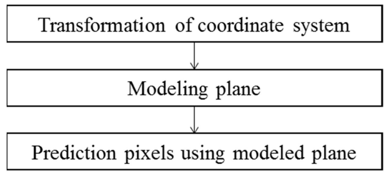
In this section, the method of intra prediction by the plane modeling is described. First, the image coordinate of each pixel in a unit block is transformed to the camera coordinate. Then, the pixel points within the block are modeled as the closest plane. The pixels are predicted using the modeled plane. The flowchart of the proposed intra prediction is shown in Figure 6.

In order to model the closest plane to pixel points in the depth picture by (6)–(8), these equations require camera coordinates. So, an image coordinate (x, y) in the picture should transform to a camera coordinate (x_c, y_c, z_c). In the depth picture, the depth is defined as the camera coordinate of z, so the depth value d is equal to z_c. Therefore, (x, y) can be transformed into (x_c, y_c, z_c) by substituting d into z_c in Equation (4):

$$\begin{array}{c}{x}_c=\frac{d}{f}x\\ y_c=\frac{d}{f}y\\ z_c=d.\end{array}$$

(9)

Finally, the pixel points are modeled from (6)–(8). The actual pixel value is predicted by substituting the modeled plane factors of (8) and the transformed camera coordinates of Equation (9) into Equation (5) as follows:

$$\tilde{P}[x,y]=-\widetilde{c_p}{\left(\frac{\widetilde{a_p}}{f}x+\frac{\widetilde{b_p}}{f}y-1\right)}^{-1},$$

(10)

where $\tilde{P}[x,y]$ stands for the predicted value in position (x, y).

H.264/AVC plane mode and H.265/HEVC planar mode calculate the Equations (1) and (3) by using the reference samples, while the proposed mode calculates the model factors using current samples in a block.

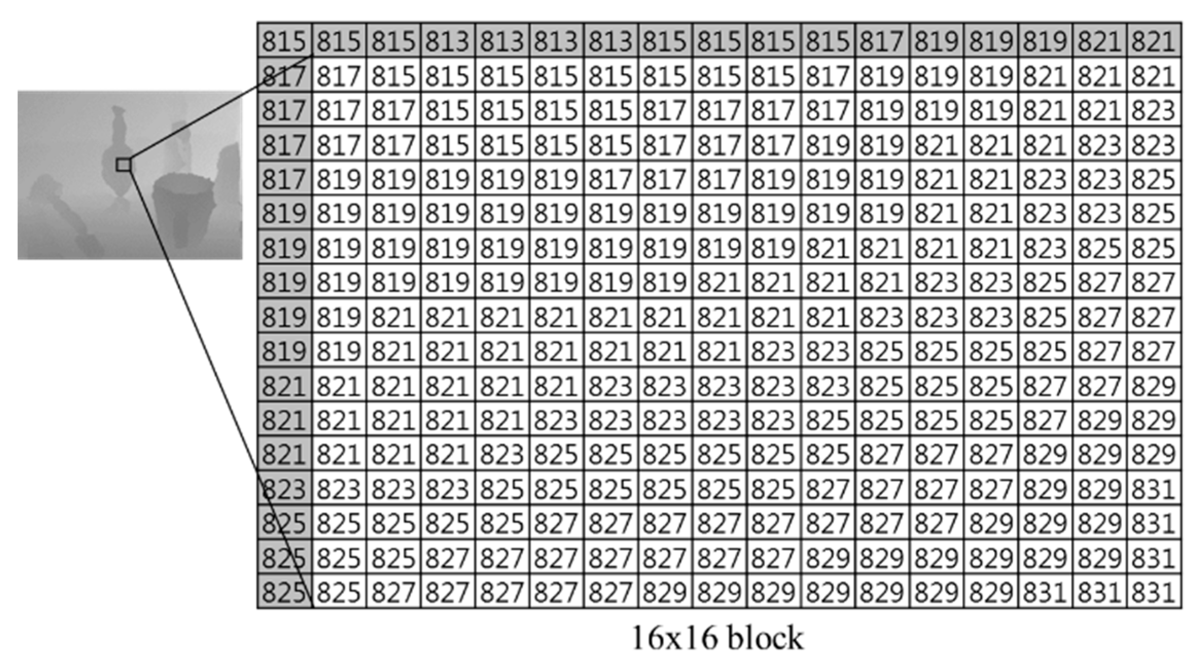
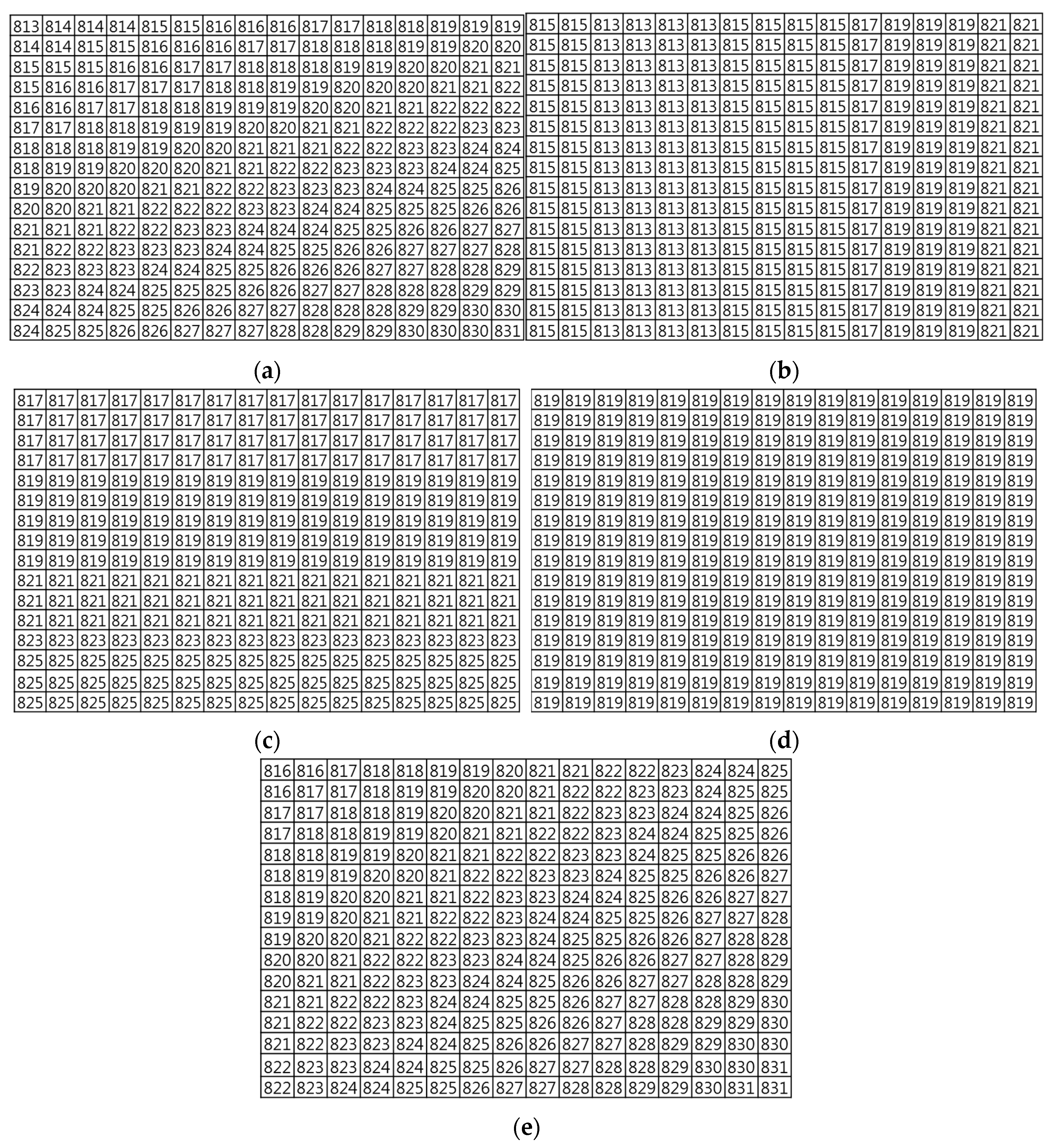
Figure 7 shows an example block for the plane modeling. From (6)–(8), $\tilde{R}$ is obtained as ${[\begin{array}{ccc}0.337& 0.191& 823\end{array}]}^{\mathrm{T}}$, and the predicted pixels by proposed mode are shown in Figure 8a. The mean square error (MSE) between the original and predicted pixels is about 1.82. The predictions for H.264/AVC are shown in Figure 8b–e. MSEs of the vertical, horizontal, DC, and plane modes are about 56.56, 12.09, 30.63, and 4.86, respectively. Therefore, we can see that the proposed prediction is better than the conventional modes for plane surface.

3.4. Intra Prediction by Plane Modeling for Variable-Size Block

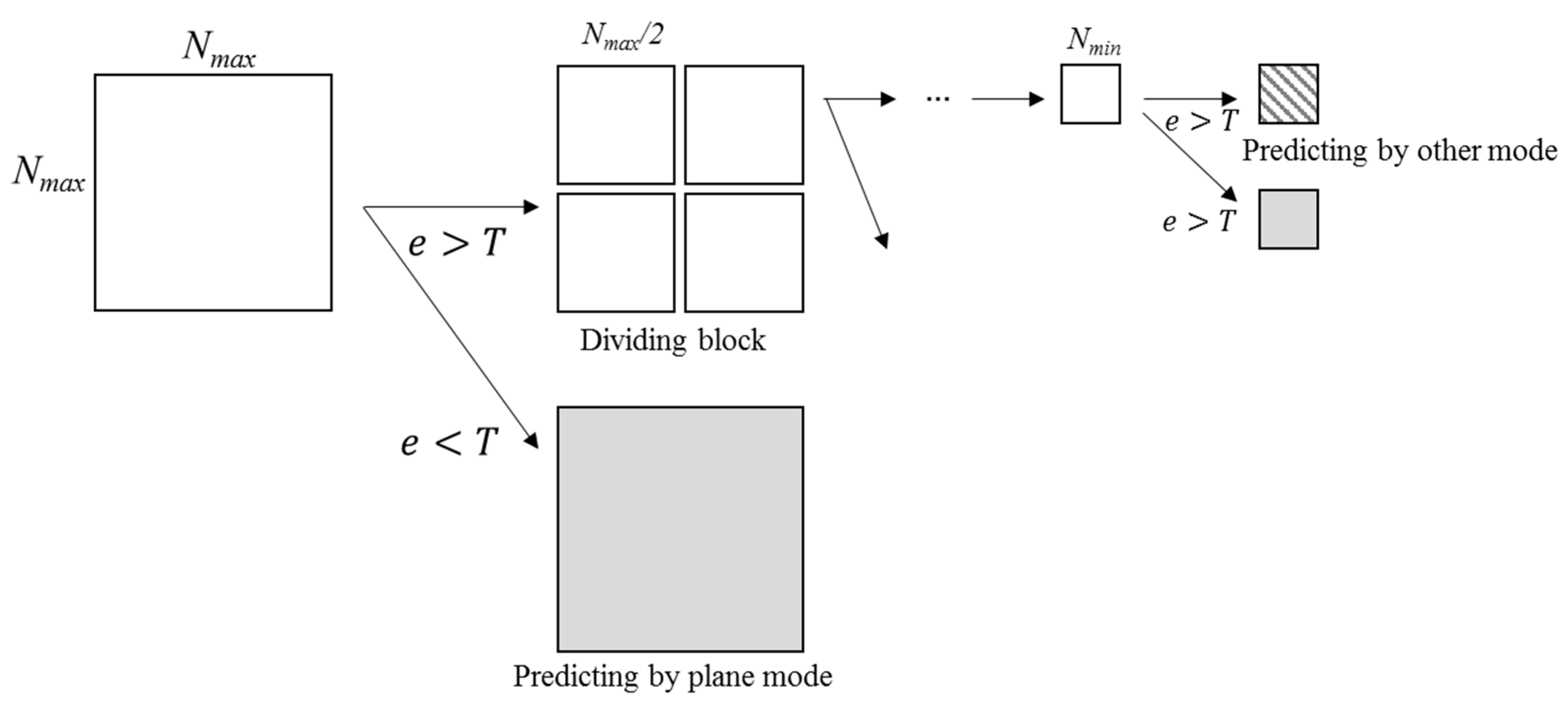
The proposed intra prediction can be available to variable-size block. First, the proposed plane modeling and prediction are performed on each block with the maximum size N_max × N_max. The predicted block is evaluated as the accuracy of the plane prediction by calculating MSE as follows:

$$\mathrm{MSE}=\frac{1}{N^2}{\sum }_{x,y}^{}{(\tilde{P}[x,y]-P[x,y])}^2,$$

(11)

where $P[x,y]$ and $\tilde{P}[x,y]$ are the original and predicted values in position (x, y), and N is the block size. If MSE is less than T, the prediction is completed with the current block size. T is a threshold. Otherwise, the block is divided by halving the width and height. The divided blocks are repeatedly modeled and predicted. If the size of a divided block is equal to minimum size N_min × N_min, the block is predicted by one of all possible modes. Figure 9 shows the process of the intra prediction for a variable-size block.

4. Simulation Results

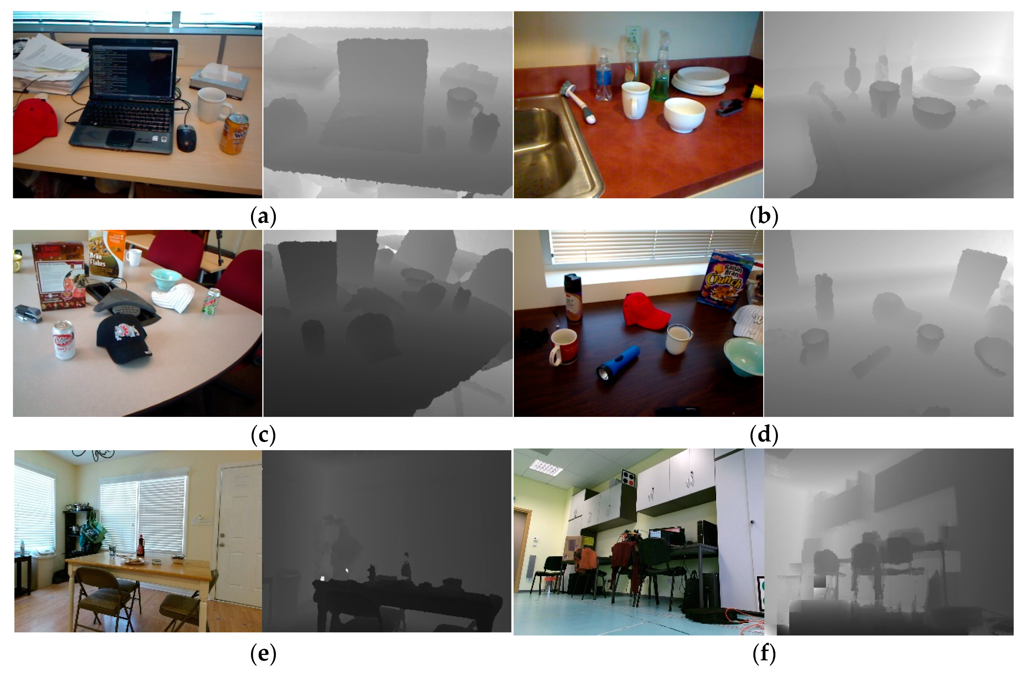
In order to measure the performance of the intra prediction, we use depth videos with various objects by Kinect and Kinect v2. The focal length of device for simulation, which is used as f in Equation (9), is specified as shown in

Table 1. Focal length of the depth camera for simulation.

Depth Camera	Focal Length
Kinect	585.6
Kinect v2	365.5

. Depth videos are obtained from [41,42,43].

Table 2. Capturing environment of the depth pictures for simulation.

Source Picture	Captured Device	Picture Resolution
desk [41]	Kinect	640 × 480
kitchen [41]	Kinect	640 × 480
meeting room [41]	Kinect	640 × 480
table [41]	Kinect	640 × 480
home [42]	Kinect v2	512 × 424
ground [43]	Kinect v2	512 × 424

shows the picture resolutions for each source. Figure 10 shows the pictures for each source.

We measure the prediction accuracy of proposed mode according to block size N. In this simulation, we regard the blocks that MSE is over than 1000 as non-plane blocks and exclude these blocks from this simulation.

Table 3. Prediction accuracy according to block size.

Source Picture	MSE
	N = 4	N = 8	N = 16	N = 32
desk	11.90	24.85	48.66	94.93
kitchen	11.16	21.00	40.10	73.88
meeting room	12.38	26.98	52.50	84.48
table	9.51	20.29	40.28	84.23
home	13.21	30.78	64.08	104.34
ground	45.78	74.87	116.30	150.19

shows the simulation results. The pixel value is predicted more accurately as N is smaller.

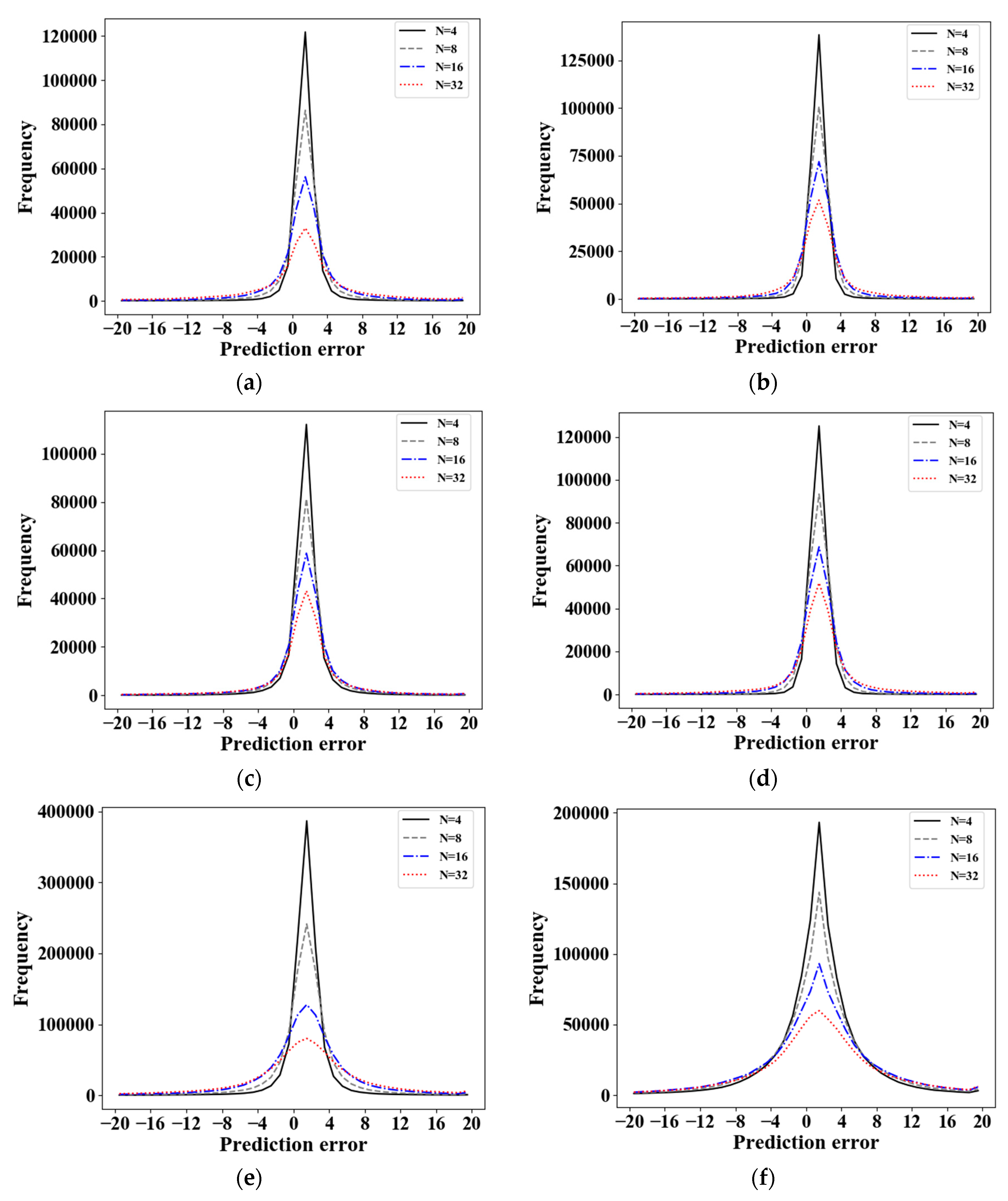
We measure distributions of the prediction error in the proposed mode. The prediction errors are distributed in the range of [−107, 105], [−226, 217], [−344, 434], and [−842, 949] in the cases of N = 4, 8, 16, and 32, respectively, as shown in

Table 4. Maximum and minimum prediction errors for proposed mode.

Source Picture	N = 4		N = 8		N = 16		N = 32
	Min	Max	Min	Max	Min	Max	Min	Max
desk	−107	103	−187	186	−326	327	−346	345
kitchen	−107	102	−169	159	−191	177	−218	204
meeting room	−106	105	−224	217	−314	328	−346	348
table	−107	104	−189	179	−238	241	−362	365
home	−99	105	−226	204	−344	342	−842	949
ground	−104	102	−178	191	−312	434	−328	446

. Figure 11 shows the distributions of prediction errors within the range of [−20,20] according to N. The variance of prediction error increases as N increases.

Next, the prediction accuracy and the entropy power are investigated when the proposed prediction mode is included. The conventional prediction modes are applied to all of the modes of H.264/AVC and the planar mode of H.265/HEVC. Including proposed mode means adding the proposed mode to the conventional modes. The entropy power is defined as the output of white noise with the same frequency of all signals in an environment. The entropy power is calculated as follows:

$$\begin{array}{c}N(X)=\frac{1}{2\pi e}{e}^{2h(X)}\\ h(X)=-{\sum }_i{f}_i\ln (f_i),\end{array}$$

(12)

where f_i is the probability of a signal i. In the results shown by

Table 5. Comparison of conventional intra prediction modes and proposed mode (Block size = 16).

Source Picture	Conventional Intra Prediction Modes (H.264/AVC + Planar Mode)		Including Proposed Mode
	MSE	Entropy Power	MSE	Entropy Power
desk	1872.30	32.41	1189.01	22.27
kitchen	451.76	24.34	199.85	10.93
meeting room	13,971.22	61.40	5471.41	38.13
table	656.07	30.69	363.60	12.37
home	123,561.65	142.12	95,058.91	69.85
ground	13,288.39	504.61	5713.84	230.13

and

Table 6. Comparison of conventional intra prediction modes and proposed mode (Block size = 4).

Source Picture	Conventional Intra Prediction Modes (H.264/AVC + Planar Mode)		Including Proposed Mode
	MSE	Entropy Power	MSE	Entropy Power
desk	287.53	1.81	219.70	1.60
kitchen	40.36	1.57	30.37	1.29
meeting room	1281.05	2.50	807.57	2.20
table	69.72	1.58	59.10	1.35
home	12,583.65	6.75	8716.85	4.14
ground	2256.50	28.62	1266.52	19.10

, prediction accuracy and entropy power are improved in the including proposed mode. These results show that the depth video can be effectively compressed by the proposed mode.

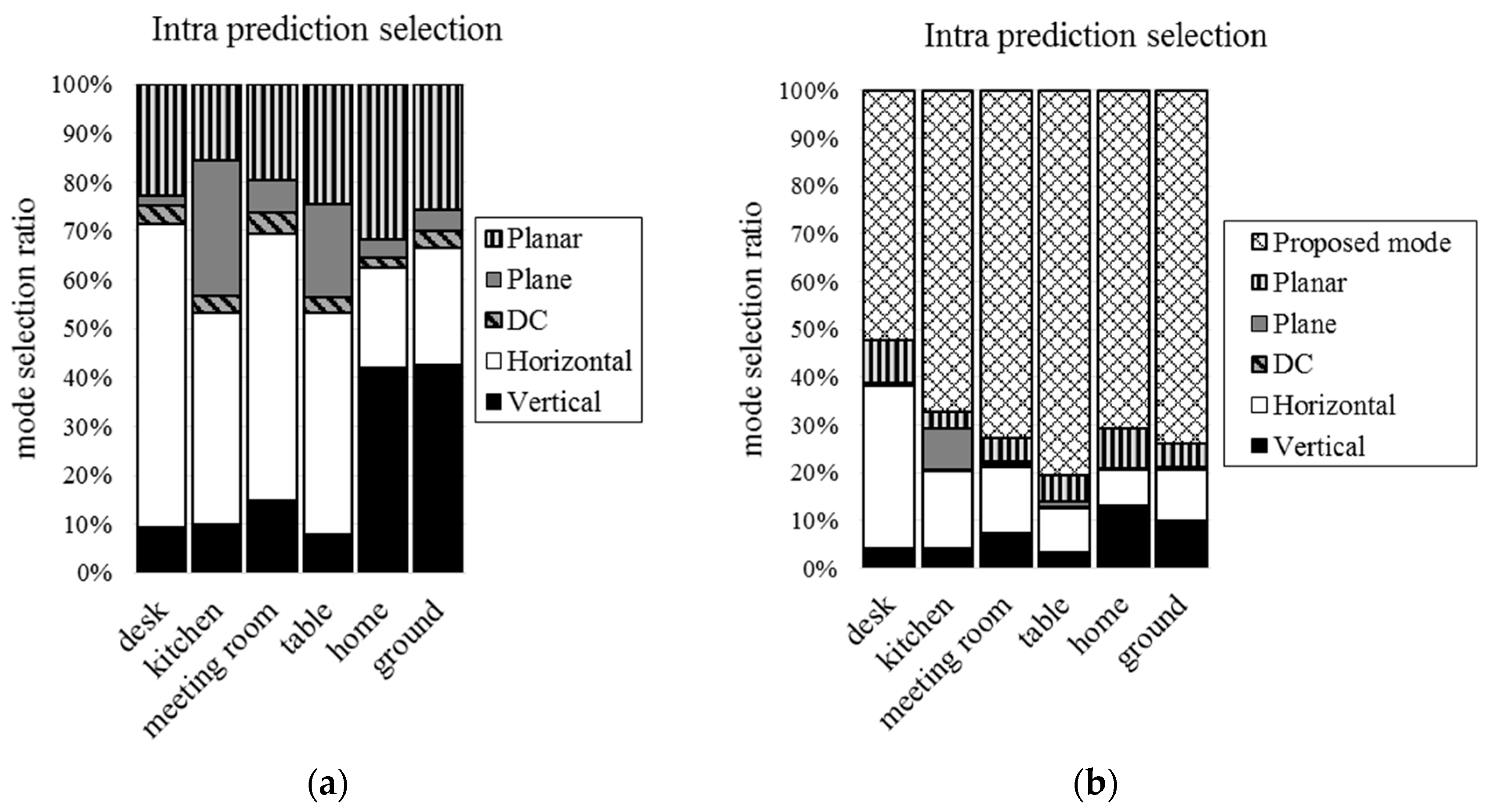
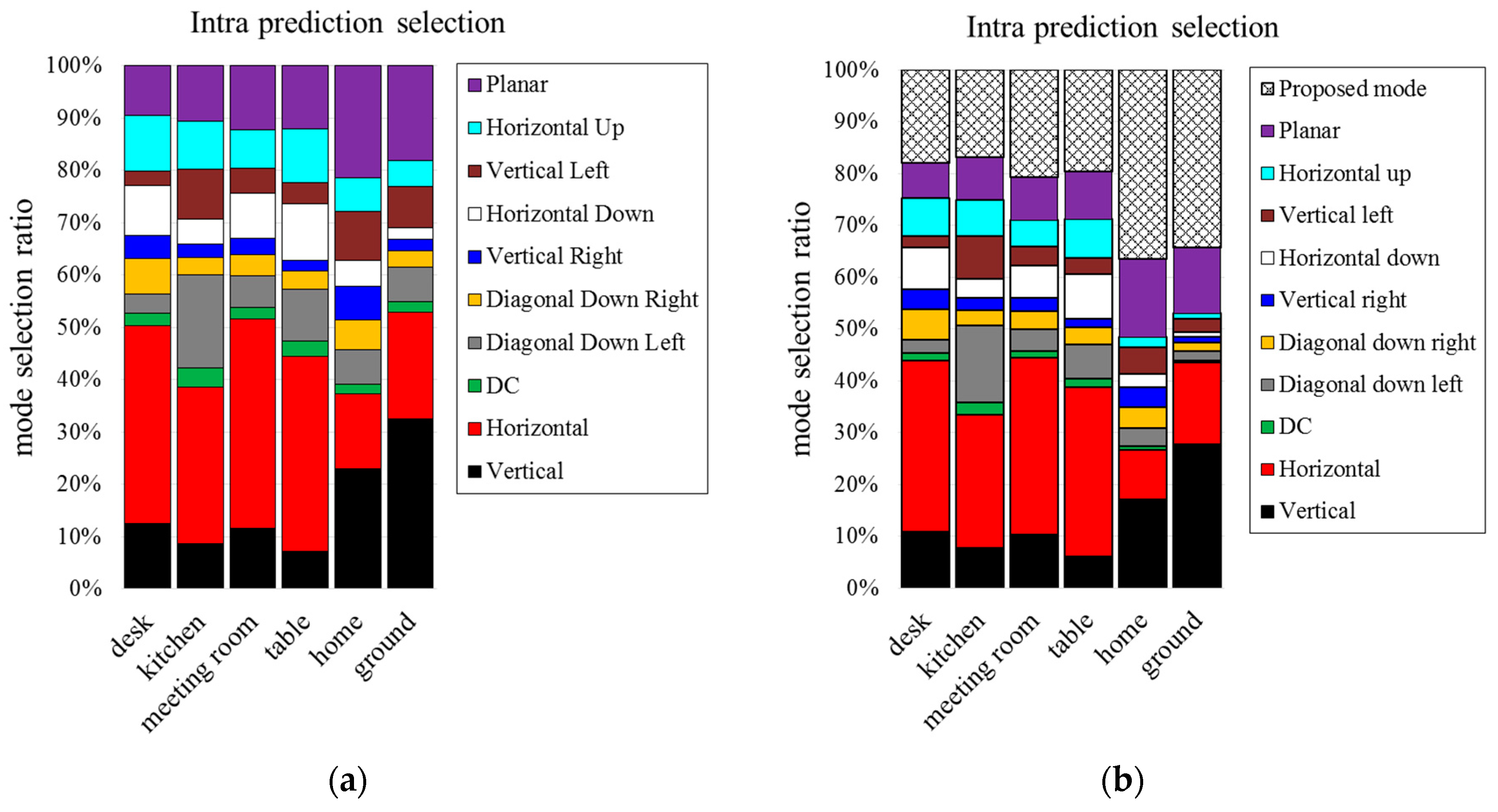
Figure 12 and Figure 13 show the mode selection frequency of intra prediction when the block sizes are 16 × 16 and 4 × 4. In the case of including the proposed mode, the proposed mode is selected by more than 50% when block size is 16 × 16. More than 20% is selected when block size is 4 × 4. We can see that the proposed mode is more efficient than conventional intra prediction modes. The proposed mode in 16 × 16 block size is selected more than 4 × 4 block size.

Then, the prediction accuracy is simulated for variable-size block. In this simulation, the minimum block size is set to 4 × 4 and the maximum block size to 32 × 32.

Table 7. MSE and number of blocks in variable-size block.

T	Desk		Kitchen		Meeting Room		Table
	MSE	Number of Blocks	MSE	Number of Blocks	MSE	Number of Blocks	MSE	Number of Blocks
100	16.30	2132	13.31	1368	14.41	2267	12.13	1469
200	27.68	1867	21.25	1179	20.04	2103	20.03	1324
300	38.77	1728	29.59	1085	28.27	1977	28.48	1197
400	49.83	1631	38.41	1020	41.58	1825	36.30	1092
500	56.38	1591	45.96	971	48.05	1760	47.86	997
600	59.54	1549	51.87	939	50.21	1743	57.34	926
700	71.69	1486	60.06	902	63.29	1676	63.31	890
800	77.60	1463	62.55	891	75.19	1621	68.70	860
900	87.29	1433	70.33	849	83.36	1589	76.62	835
1000	92.13	1410	83.19	803	93.76	1541	89.67	806

shows the number of blocks divided by variable-size and MSE according to threshold T. The prediction accuracy is improved as the T is lower, but the number of blocks increases as the T is lower.

Table 8. Number of blocks by size in variable-size block in ‘desk’.

Block Size	T
	200	400	600	800
32 × 32	184	204	208	215
16 × 16	240	192	186	170
8 × 8	441	381	373	349
4 × 4	1002	854	782	733
Non proposed mode selected (4 × 4)	818	694	638	591

,

Table 9. Number of blocks by size in variable-size block in ‘kitchen’.

Block Size	T
	200	400	600	800
32 × 32	230	245	251	254
16 × 16	154	117	109	107
8 × 8	259	222	187	167
4 × 4	536	436	392	363
Non proposed mode selected (4 × 4)	444	324	252	201

,

Table 10. Number of blocks by size in variable-size block in ‘meeting room’.

Block Size	T
	200	400	600	800
32 × 32	183	197	199	208
16 × 16	200	187	192	173
8 × 8	529	437	414	379
4 × 4	1191	1004	938	861
Non proposed mode selected (4 × 4)	981	848	798	743

and

Table 11. Number of blocks by size in variable-size block in ‘table’.

Block Size	T
	200	400	600	800
32 × 32	226	238	250	253
16 × 16	148	135	111	109
8 × 8	316	245	185	167
4 × 4	634	474	380	331
Non proposed mode selected (4 × 4)	470	354	304	265

show the number of blocks according to the block size when the threshold T is 200, 400, 600, and 800, respectively. As T is larger, the number of blocks which are selected to the maximum block size increases and the number of blocks which are selected to others block sizes decreases.

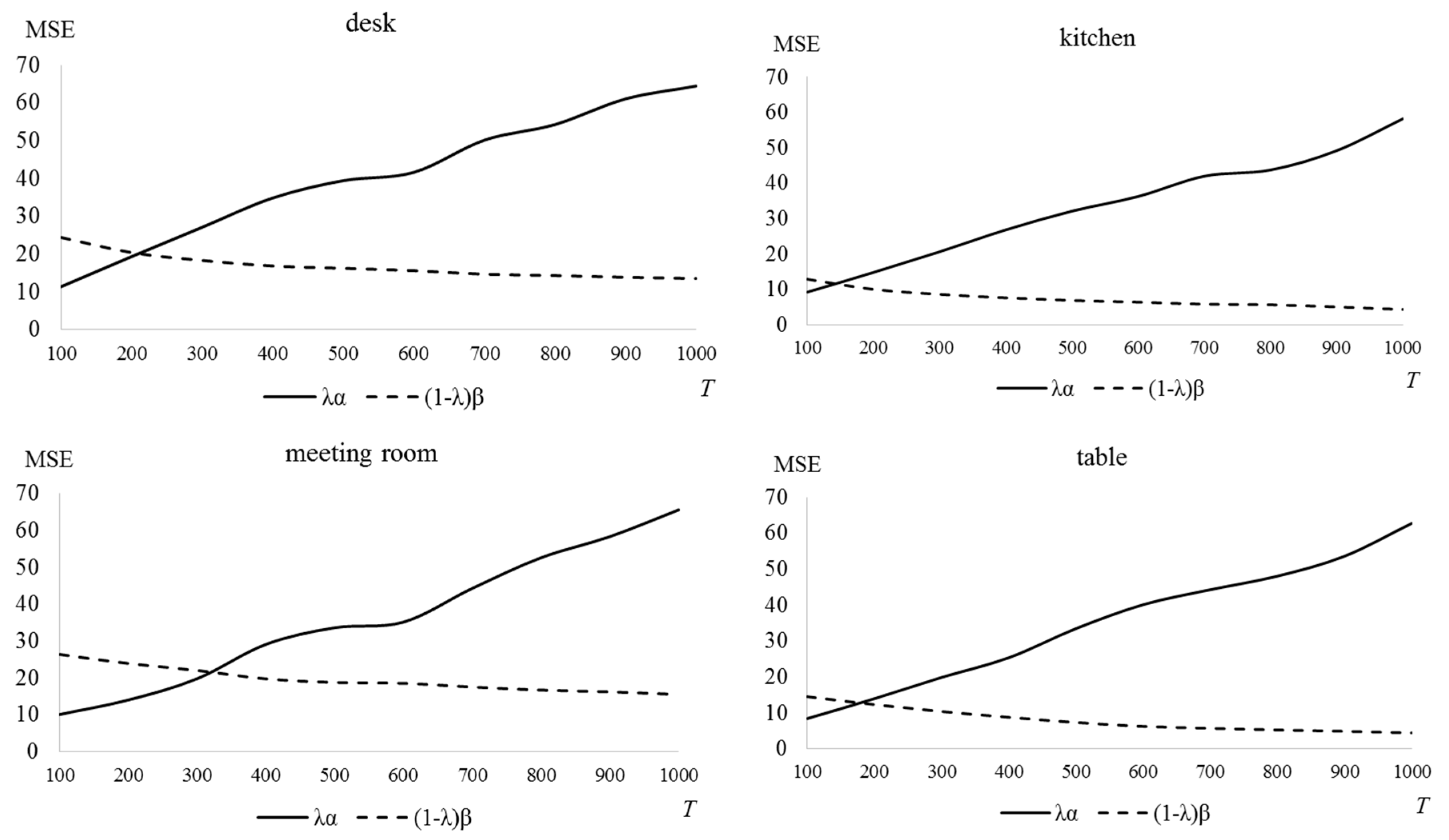
The encoding efficiency increases as the number of blocks divided by variable-size decreases. It is necessary to select optimal T in consideration of the inverse relationship between the prediction accuracy and the encoding efficiency. To find the optimal T, we define ${\alpha }_T$ and ${\beta }_T$ as:

$$\begin{array}{c}{\alpha }_T={\mathrm{MSE}}_T\\ {\beta }_T=(B_T-500)/(2500-500)\times 100,\end{array}$$

(13)

where ${\alpha }_T$ is MSE described in (11), ${\beta }_T$ is the number of blocks divided by variable-size according to T. The optimal T is determined by finding a solution that satisfies the following equation:

$$\lambda {\alpha }_T-(1-\lambda ){\beta }_T=0, (0\le \lambda \le 1),$$

(14)

where λ is a parameter that the weight between the prediction accuracy and the number of blocks divided by variable-size. Figure 14 shows finding the optimal T in each picture when λ = 0.7. In this case, the optimal T is determined between 150 and 300.

5. Conclusions

In this paper, the intra prediction method was proposed for the depth picture coding by the plane modeling. The variable-size block was also proposed in intra prediction. The proposed method predicts the pixels based on a plane model by transforming the coordinates into 3D using the depth value. The accuracy was improved by proposed prediction which was suitable for the characteristic of the depth picture. The proposed mode has an advantage that the value can be predicted more effectively than the conventional method for a rolled or tilted plane. In the proposed intra prediction mode, the model factors of each plane are required to coding process. A method of encoding the model factors for each plane should be further researched.

References

- Song, S.; Xiao, J. Tracking revisited using RGBD camera: Unified benchmark and baselines. In Proceedings of the IEEE International Conference on Computer Vision, Sydney, Australia, 1–8 December 2013; pp. 233–240. [Google Scholar]
- Fanelli, G.; Dantone, M.; Van Gool, L. Real time 3D face alignment with random forests-based active appearance models. In Proceedings of the IEEE International Conference and Workshops on Automatic Face and Gesture Recognition, Shanghai, China, 22–26 April 2013; pp. 1–8. [Google Scholar]
- Dantone, M.; Gall, J.; Fanelli, G.; Van Gool, L. Real-time facial feature detection using conditional regression forests. In Proceedings of the IEEE International Conference and Workshops on Computer Vision and Pattern Recognition, Providence, RI, USA, 16–21 June 2012; pp. 2578–2585. [Google Scholar]
- Min, R.; Kose, N.; Dugelay, J.L. KinectFaceDB: A Kinect Database for Face Recognition Systems. IEEE Trans. Man Cybern. Syst. 2014, 44, 1534–1548. [Google Scholar] [CrossRef]
- Sung, J.; Ponce, C.; Selman, B.; Saxena, A. Human Activity Detection from RGBD Images. Plan Act. Intent Recognit. 2011, 64, 47–55. [Google Scholar]
- Spinello, L.; Arras, K.O. People detection in RGB-D data. In Proceedings of the IEEE/RSJ International Conference on Intelligent Robots and Systems, San Francisco, CA, USA, 25–30 September 2011; pp. 3838–3843. [Google Scholar]
- Luber, M.; Spinello, L.; Arras, K.O. People tracking in RGB-D data with on-line boosted target models. In Proceedings of the IEEE/RSJ International Conference on Intelligent Robots and Systems, San Francisco, CA, USA, 25–30 September 2011; pp. 3844–3849. [Google Scholar]
- Sturm, J.; Engelhard, N.; Endres, F.; Burgard, W.; Cremers, D. A benchmark for the evaluation of RGB-D SLAM systems. In Proceedings of the IEEE/RSJ International Conference on Intelligent Robots and Systems, Vilamoura, Portugal, 7–12 October 2012; pp. 573–580. [Google Scholar]
- Pomerleau, F.; Magnenat, S.; Colas, F.; Liu, M.; Siegwart, R. Tracking a depth camera: Parameter exploration for fast ICP. In Proceedings of the IEEE/RSJ International Conference on Intelligent Robots and Systems, San Francisco, CA, USA, 25–30 September 2011; pp. 3824–3829. [Google Scholar]
- Gumhold, S.; Karni, Z.; Isenburg, M.; Seidel, H. Predictive pointcloud compression. In Proceedings of the ACM SIGGRAPH, Los Angeles, CA, USA, 31 July–4 August 2005; pp. 137–141. [Google Scholar]
- Kammerl, J.; Blodow, N.; Rusu, R.B.; Gedikli, S.; Beetz, M.; Steinbach, E. Real-time Compression of Point Cloud Streams. In Proceedings of the IEEE International Conference on Robotics and Automation, Saint Paul, MN, USA, 14–18 May 2012; pp. 778–785. [Google Scholar]
- Devillers, O.; Gandoin, P. Geometric compression for interactive transmission. In Proceedings of the International Conference on Information Visualization, Salt Lake City, UT, USA, 8–13 October 2000; pp. 319–326. [Google Scholar]
- Peng, J.; Kuo, C. Octree-based progressive geometry encoder. In Proceedings of the SPIE, Orlando, FL, USA, 7–11 September 2003; pp. 301–311. [Google Scholar]
- Huang, Y.; Peng, J.; Kuo, C.; Gopi, M. Octree-based progressive geometry coding of point clouds. In Proceedings of the Eurographics Symposium on Point-Based Graphics, Boston, MA, USA, 29–30 July 2006; pp. 103–110. [Google Scholar]
- Schnabel, R.; Klein, R. Octree-based point-cloud compression. In Proceedings of the Eurographics Symposium on Point-Based Graphics, Boston, MA, USA, 29–30 July 2006; pp. 111–120. [Google Scholar]
- Tekalp, A.M.; Ostermann, J. Face and 2-D mesh animation in MPEG-4. Signal Process. Image Commun. 2000, 15, 387–421. [Google Scholar] [CrossRef] [Green Version]
- Mamou, K.; Zaharia, T.; Prêteux, F. FAMC: The MPEG-4 standard for animated mesh compression. In Proceedings of the IEEE International Conference on Image Processing, San Diego, CA, USA, 12–15 October 2008; pp. 2676–2679. [Google Scholar]
- Touma, C.; Gotsman, C. Triangle mesh compression. Proc. Graph. Interface 1998, 98, 26–34. [Google Scholar]
- Karni, Z.; Gotsman, C. Spectral compression of mesh geometry. In Proceedings of the 27th Annual Conference on Computer Graphics and Interactive Techniques, New Orleans, LA, USA, 23–28 July 2000; pp. 279–286. [Google Scholar]
- Grewatsch, S.; Muller, E. Fast mesh-based coding of depth map sequences for efficient 3D video reproduction using openGL. In Proceedings of the International Conference on Visualization, Imaging and Image Processing, Benidorm, Spain, 7–9 September 2005; pp. 66–71. [Google Scholar]
- Chai, B.B.; Sethuraman, S.; Sawhney, H.S.; Hatrack, P. Depth map compression for real-time view-based rendering. Pattern Recognit. Lett. 2004, 25, 755–766. [Google Scholar] [CrossRef]
- Fu, J.; Miao, D.; Yu, W.; Wang, S.; Lu, Y.; Li, S. Kinect-Like Depth Data Compression. IEEE Trans. Multimed. 2013, 15, 1340–1352. [Google Scholar] [CrossRef]
- Grewatsch, S.; Muller, E. Evaluation of motion compensation and coding strategies for compression of depth map sequences. In Proceedings of the Mathematics of Data/Image Coding, Compression, and Encryption VII, with Applications, Denver, CO, USA, 2–6 August 2004; pp. 117–125. [Google Scholar]
- Morvan, Y.; Farin, D.; de With, P.H.N. Depth-image compression based on an R-D optimized quadtree decomposition for the transmission of multiview images. In Proceedings of the IEEE International Conference on Image Processing, San Antonio, TX, USA, 16–19 September 2007; pp. V-105–V-108. [Google Scholar]
- Milani, S.; Calvagno, G. A depth image coder based on progressive silhouettes. IEEE Signal Process. Lett. 2010, 17, 711–714. [Google Scholar] [CrossRef]
- Shen, G.; Kim, W.; Narang, S.; Orterga, A.; Lee, J.; Wey, H. Edge adaptive transform for efficient depth map coding. In Proceedings of the Picture Coding Symposium, Nagoya, Japan, 8–10 December 2010; pp. 566–569. [Google Scholar]
- Maitre, M.; Do, M. Depth and depth-color coding using shape adaptive wavelets. J. Vis. Commun. Image Represent. 2010, 21, 513–522. [Google Scholar] [CrossRef]
- Hartley, R.; Zisserman, A. Multiple View Geometry in Computer Vision; Cambridge University Press: Cambridge, UK, 2008; ISBN 9780521540513. [Google Scholar]
- Liu, S.; Lai, P.; Tian, D.; Chen, C.W. New depth coding techniques with utilization of corresponding video. IEEE Trans. Broadcast. 2011, 57, 551–561. [Google Scholar] [CrossRef]
- Lan, C.; Xu, J.; Wu, F. Object-based coding for Kinect depth and color videos. In Proceedings of the Visual Communications and Image Processing, San Diego, CA, USA, 27–30 November 2012; pp. 1–6. [Google Scholar]
- Shen, G.; Kim, W.S.; Ortega, A.; Lee, J.; Wey, H. Edge-aware intra prediction for depth-map coding. In Proceedings of the IEEE International Conference on Image Processing, Hong Kong, China, 26–29 September 2010; pp. 3393–3396. [Google Scholar]
- H.264: Advanced Video Coding for Generic Audiovisual Services. ITU-T Rec. H.264. Available online: https://www.itu.int/rec/T-REC-H.264/en (accessed on 10 November 2018).
- Richardson, I.E.G. H.264 and MPEG-4 Video Compression: Video Coding for Next-Generation Multimedia; Wiley: Hoboken, NJ, USA, 2003; ISBN 9780470848371. [Google Scholar]
- Wiegand, T.; Sullivan, G.J.; Bjonttegaard, G.; Luthra, A. Overview of the H.264/AVC video coding standard. IEEE Trans. Circuits Syst. Video Technol. 2003, 13, 560–576. [Google Scholar] [CrossRef] [Green Version]
- Kwon, S.K.; Tamhankar, A.; Rao, K.R. Overview of H.264/MPEG-4 part 10. J. Vis. Commun. Image Represent. 2006, 17, 186–216. [Google Scholar] [CrossRef]
- Kwon, S.K.; Punchihewa, A.; Bailey, D.G.; Kim, S.W.; Lee, J.H. Adaptive simplification of prediction modes for H.264 intra-picture coding. IEEE Trans. Broadcast. 2012, 58, 125–129. [Google Scholar] [CrossRef]
- Sullivan, G.J.; Ohm, J.; Han, W.J.; Wiegand, T. Overview of the high efficiency video coding (HEVC) standard. IEEE Trans. Circuits Syst. Video Technol. 2012, 22, 1649–1668. [Google Scholar] [CrossRef]
- Patel, D.; Lad, T.; Shah, D. Review on Intra-prediction in High Efficiency Video Coding (HEVC) Standard. Int. J. Comput. Appl. 2015, 132, 26–29. [Google Scholar] [CrossRef]
- Ugur, K.; Andersson, K.R.; Fuldseth, A. JCTVC-A119: Description of Video Coding Technology Proposal by Tandberg, Nokia, Ericsson. In Proceedings of the 1st Meeting of Joint Collaborative Team on Video Coding (JCT-VC), Dresden, DE, USA, 15–23 April 2010. [Google Scholar]
- Kanumuri, S.; Tan, T.K.; Bossen, F. JCTVC-D235: Enhancements to Intra Coding. In Proceedings of the 4th Meeting of Joint Collaborative Team on Video Coding (JCT-VC), Daegu, Korea, 20–28 January 2011. [Google Scholar]
- Lai, K.; Bo, L.; Ren, X.; Fox, D. A large-scale hierarchical multi-view RGB-D object dataset. In Proceedings of the IEEE International Conference on Robotics and Automation, Shanghai, China, 9–13 May 2011; pp. 1817–1824. [Google Scholar]
- Ammirato, P.; Poirson, P.; Park, E.; Košecká, J.; Berg, A.C. A dataset for developing and benchmarking active vision. In Proceedings of the IEEE International Conference on Robotics and Automation, Singapore, 29 May–3 June 2017; pp. 1378–1385. [Google Scholar]
- Kraft, M.; Nowicki, M.; Schmidt, A.; Fularz, M.; Skrzypczyński, P. Toward evaluation of visual navigation algorithms on RGB-D data from the first- and second-generation Kinect. Mach. Vis. Appl. 2016, 28, 61–74. [Google Scholar] [CrossRef]
Figure 1.
Intra prediction pixels and prediction directions for 4 × 4 luma block.
Figure 2.
Intra prediction directions of H.265/HEVC.
Figure 3.
Planar mode in intra prediction of H.265/HEVC.
Figure 4.
Planar + DST mode.
Figure 5.
The pinhole camera model: (a) 3D geometry; and (b) geometry projected on YZ-plane.
Figure 6.
Flowchart of the proposed method.
Figure 7.
Example block for plane modeling.
Figure 8.
Comparison of proposed prediction mode and prediction mode in H.264/AVC for Figure 7: (a) proposed mode; (b) vertical mode; (c) horizontal mode; (d) DC mode; and (e) plane mode.
Figure 9.
Intra prediction for a variable-size block.
Figure 10.
Depth pictures for simulation: (a) desk; (b) kitchen; (c) meeting room; (d) table; (e) home; and (f) ground.
Figure 11.
Distributions of prediction errors: (a) desk; (b) kitchen; (c) meeting room; (d) table; (e) home; and (f) ground.
Figure 12.
Selection ratio for 16 × 16 block size: (a) conventional intra prediction modes; and (b) including proposed mode.
Figure 13.
Selection ratio for 4 × 4 block size: (a) conventional intra prediction modes; and (b) including proposed mode.
Figure 14.
Determining optimal T in variable-size block (λ = 0.7).