Symmetry Reduction and Numerical Solution of Von K a ´ rm a ´ n Swirling Viscous Flow

Abstract

In this paper, the numerical solutions of von K$\acute{a}$rm$\acute{a}$n swirling viscous flow are obtained based on the effective combination of the symmetry method and the Runge-Kutta method. Firstly, the multi-parameter symmetry of von K$\acute{a}$rm$\acute{a}$n swirling viscous flow is determined based on the differential characteristic set algorithm. Secondly, we used the symmetry to reduce von K$\acute{a}$rm$\acute{a}$n swirling viscous flow to an initial value problem of the original differential equations. Finally, we numerically solve the initial value problem of the original differential equations by using the Runge-Kutta method.

1. Introduction

The symmetry group method is very important in the analysis of partial differential equations (PDEs), and this method is applied widely in many field [1,2,3]. The applications of Lie’s continuous symmetry groups include such diverse fields as differential geometry, bifurcation theory, mechanics, hydrodynamics, relativity, diffusion and wave phenomena, astrophysics, plasma and so on [3,4,5,6,7]. There have been several studies about the symmetry method, such as symmetry classification [8], potential symmetry [9], approximate symmetry [10], etc. Based on the symmetries of a PDE, many important properties of the equation such as Lie algebras [11,12], conservation laws [13,14,15,16,17,18], and exact solutions [16,17,18,19,20,21,22] can be considered successively. Recently, some researchers focus on the applications of the symmetry method for solving boundary value problems (BVP) of a PDE [2,23,24,25].

As it is well known, the similarity transformation is used frequently in solving nonlinear PDEs problems. The Lie transformation group of PDEs can yield a more general form of similarity transformation, and these transformations have more significance for mathematics and physics. So the symmetry method has a higher superiority than the similarity transformation in BVP of nonlinear PDEs. At present, combining the symmetry method with other methods to solve BVP of the nonlinear PDEs are the new research subjects. Recently, we have studied this topic based on the differential characteristic set algorithm [26,27,28].

It is an new research to the application of the Lie symmetry method in the BVP for nonlinear PDEs in fluid mechanics. We will study the symmetry reduction and the numerical solutions of von K$\acute{a}$rm$\acute{a}$n swirling viscous flow based on the effective combination of the Lie symmetry method and the Runge-Kutta method. This investigation will widen the application of Lie symmetry. The rest of the paper is organized as follows. In Section 2, we give the formulation of invariance for a BVP of PDEs. In Section 3, we obtain the symmetry of von K$\acute{a}$rm$\acute{a}$n swirling viscous flow based on the differential characteristic set algorithm and then we reduce it. In Section 4, we give numerical solutions of von K$\acute{a}$rm$\acute{a}$n swirling viscous flow by applying the Runge-Kutta method. In Section 5, we give a discussion and conclusion remarks.

2. Formulation of Invariance for a BVP of PDEs

Consider a BVP for kth order scalar PDEs $(k\ge 2)$

$$\begin{array}{c}\hfill F^{\mu }(x,u,\partial u,{\partial }^{2}u,\dots ,{\partial }^{k}u)=u_{i_1,i_2,\cdots ,i_l}-f^{\mu }(x,u,\partial u,{\partial }^{2}u,\dots ,{\partial }^{k}u)=0,\end{array}$$

(1)

(where $f^{\mu }(x,u,\partial u,{\partial }^{2}u,\dots ,{\partial }^{k}u)$ does not depend on $u_{i_1,i_2,\cdots ,i_l}$) where $x=(x_1,x_2,\cdots ,x_n)$ are n independent variables, $u=(u^1,u^2,\cdots ,u^m)$ are m dependent variables and defined on a domain ${\mathsf{\Omega }}_x$ in x-space with boundary conditions

$$\begin{array}{c}\hfill B_{\alpha }^{\nu }(x,u,\partial u,{\partial }^{2}u,\dots ,{\partial }^{k-1}u)=0,\nu =1,2,\cdots ,m\end{array}$$

(2)

prescribed on boundary surfaces

$$\begin{array}{c}\hfill {\omega }_{\alpha }\left(x\right)=0,\alpha =1,2,\cdots ,s.\end{array}$$

(3)

Assume that BVP (1)–(3) has a unique solution. Consider an infinitesimal generator of the form

$$\begin{array}{c}\hfill X={\xi }_i(x,u)\frac{\partial }{\partial x_i}+{\eta }^{\nu }(x,u)\frac{\partial }{\partial u_{\nu }},i=1,2,\cdots ,n;\nu =1,2,\cdots ,m.\end{array}$$

(4)

which defines a one-parameter Lie group of transformations in x-space as well as in $(x,u)$-space.

Definition 1.

X is admitted by BVP (1)–(3) if and only if [2]

$$\begin{array}{c}\hfill X^{\left(k\right)}F(x,u,\partial u,{\partial }^{2}u,\dots ,{\partial }^{k}u)=0,\mathit{when}F(x,u,\partial u,{\partial }^{2}u,\dots ,{\partial }^{k}u)=0;\end{array}$$

(5)

$$\begin{array}{c}\hfill X{\omega }_{\alpha }\left(x\right)=0,\mathit{when}{\omega }_{\alpha }\left(x\right)=0,\alpha =1,2,\cdots ,s;\end{array}$$

(6)

$$\begin{array}{c}{X}^{\left(k-1\right)}{B}_{\alpha }^{\nu }(x,u,\partial u,{\partial }^{2}u,\dots ,{\partial }^{k-1}u)=0,\mathit{when}{B}_{\alpha }^{\nu }(x,u,\partial u,{\partial }^{2}u,\dots ,{\partial }^{k-1}u)=0,{\omega }_{\alpha }\left(x\right)=0,\\ \alpha =1,2,\cdots ,s\end{array}$$

(7)

where $X^{\left(k\right)}$ is kth $(k\ge 1)$ extended infinitesimal generator of X given by

$$\begin{array}{c}{X}^{\left(k\right)}={\xi }_i(x,u)\frac{\partial }{\partial x_i}+{\eta }^{\nu }(x,u)\frac{\partial }{\partial u^{\nu }}+{\eta }_i^{\left(1\right)\nu }(x,u,\partial u)\frac{\partial }{\partial u_i^{\nu }}+\cdots \\ +{\eta }_{i_1{i}_2\cdots i_k}^{\left(k\right)\nu }(x,u,\partial u,{\partial }^{2}u,\cdots ,{\partial }^{k}u)\frac{\partial }{\partial u_{i_1{i}_2\cdots i_k}^{\nu }},\end{array}$$

(8)

$$\begin{array}{c}{\displaystyle u_i^{\nu }=\frac{\partial u^{\nu }}{\partial x_i},{\eta }_i^{\left(1\right)\nu }=D_i{\eta }^{\nu }-\left(D_i{\xi }_j\right)u_j^{\nu },{\eta }_{i_1{i}_2\cdots i_t}^{\left(t\right)\nu }=D_{i_t}{\eta }_{i_1{i}_2\cdots i_{t-1}}^{(t-1)\nu }-{\left(D_{i_t}{\xi }_j\right)}_{i_1{i}_2\cdots i_{t-1}j}^{\nu },}\end{array}$$

(9)

$$\begin{array}{c}{\displaystyle D_i=\frac{\partial }{\partial x_i}+u_i^{\nu }\frac{\partial }{\partial u^{\nu }}+u_{ij}^{\nu }\frac{\partial }{\partial u_j^{\nu }}+\cdots +u_{i{i}_1{i}_2\cdots i_n}^{\nu }\frac{\partial }{\partial u_{i_1{i}_2\cdots i_n}^{\nu }}+\cdots ,}\end{array}$$

(10)

and $i=1,2,\cdots ,n;\nu =1,2,\cdots ,m;i_{\ell }=1,2,\cdots ,n;\ell =1,2,\cdots ,t,t\ge 2.$

3. The Symmetry and Symmetry Reduction of von K$\acute{a}$rm$\acute{a}$n sWirling Viscous Flow

Let us consider von K$\acute{a}$rm$\acute{a}$n swirling viscous flow which is a famous classical problem in fluid mechanics. The governing equations are as follows:

$$\begin{array}{c}\frac{1}{r}\frac{\partial \left(r{V}_r\right)}{\partial r}+\frac{1}{r}\frac{\partial V_{\theta }}{\partial \theta }+\frac{\partial V_z}{\partial z}=0,\hfill \end{array}$$

(11)

$$\begin{array}{c}{V}_r\frac{\partial V_r}{\partial r}+V_z\frac{\partial V_r}{\partial z}-\frac{V_{\theta }^2}{r}=\nu \left(\frac{{\partial }^2{V}_r}{\partial r^2}+\frac{1}{r}\frac{\partial V_r}{\partial r}+\frac{{\partial }^2{V}_r}{\partial z^2}-\frac{V_r}{r^2}\right)-\frac{1}{\rho }\frac{\partial p}{\partial r},\hfill \end{array}$$

(12)

$$\begin{array}{c}{V}_r\frac{\partial V_{\theta }}{\partial r}+V_z\frac{\partial V_{\theta }}{\partial z}+\frac{V_r{V}_{\theta }}{r}=\nu \left(\frac{{\partial }^2{V}_{\theta }}{\partial r^2}+\frac{1}{r}\frac{\partial V_{\theta }}{\partial r}+\frac{{\partial }^2{V}_{\theta }}{\partial z^2}-\frac{V_{\theta }}{r^2}\right),\hfill \end{array}$$

(13)

$$\begin{array}{c}{V}_r\frac{\partial V_z}{\partial r}+V_z\frac{\partial V_z}{\partial z}=\nu \left(\frac{{\partial }^2{V}_z}{\partial r^2}+\frac{1}{r}\frac{\partial V_z}{\partial r}+\frac{{\partial }^2{V}_z}{\partial z^2}\right)-\frac{1}{\rho }\frac{\partial p}{\partial z},\hfill \end{array}$$

(14)

where $V_r,V_{\theta },V_z,p$ are all functions of $r,\theta ,z$. $\rho$ is the fluid density, $\nu$ is the kinematic viscosity, p is the pressure. The boundary conditions of Equations (11)–(14) are

$$\begin{array}{c}{V}_r(r,\theta ,0)=B_1(r,\theta ),V_{rz}(r,\theta ,0)=B_2(r,\theta ),V(r,\theta ,+\infty )=0,\hfill \end{array}$$

(15)

$$\begin{array}{c}{V}_{\theta }(r,\theta ,0)=B_3(r,\theta ),V_{\theta z}(r,\theta ,0)=B_4(r,\theta ),V(r,\theta ,+\infty )=0,\hfill \end{array}$$

(16)

$$\begin{array}{c}{V}_z(r,\theta ,0)=B_5(r,\theta ),V_{zz}(r,\theta ,0)=B_6(r,\theta ),\hfill \end{array}$$

(17)

$$\begin{array}{c}p(r,\theta ,0)=B_7(r,\theta ),p_z(r,\theta ,0)=B_8(r,\theta ),\hfill \end{array}$$

(18)

where $U_{rz}=\partial U_r/\partial z,U_{\theta z}=\partial U_{\theta }/\partial z,U_{zz}=\partial U_z/\partial z,$ and $B_i(r,\theta )(i=1,\cdots ,8)$ are the functions of $(r,\theta )$ to be determined later.

3.1. First Symmetry Reduction

The symmetry group of Equations (11)–(14) will be generated by the vector field of the form

$$\begin{array}{c}\hfill X_1={\xi }_1\frac{\partial }{\partial r}+{\xi }_2\frac{\partial }{\partial \theta }+{\xi }_3\frac{\partial }{\partial z}+{\eta }_1\frac{\partial }{\partial V_r}+{\eta }_2\frac{\partial }{\partial V_{\theta }}+{\eta }_3\frac{\partial }{\partial V_z}+{\eta }_4\frac{\partial }{\partial p},\end{array}$$

(19)

where ${\xi }_i={\xi }_i(r,\theta ,z,V_r,V_{\theta },V_z,p),{\eta }_j={\eta }_j(r,\theta ,z,V_r,V_{\theta },V_z,p)$ are the infinitesimal functions of the symmetry.

We obtain the determining equations of symmetry (19) by using the Lie algorithm, but it is too difficult to get their solutions. However, we use the differential characteristic set algorithm to obtain the following equivalent system of the determining equations [29].

$$\begin{array}{c}{\xi }_{1\theta }={\xi }_{1z}={\xi }_{1V_r}={\xi }_{1V_{\theta }}={\xi }_{1V_z}={\xi }_{1p}=0,{\xi }_{2r}={\xi }_{2\theta }={\xi }_{2z}={\xi }_{2V_r}={\xi }_{2V_{\theta }}={\xi }_{2V_z}={\xi }_{2p}=0,\hfill \\ {\xi }_{3r}={\xi }_{3\theta }={\xi }_{3V_r}={\xi }_{3V_{\theta }}={\xi }_{3V_z}={\xi }_{3p}=0,{\eta }_{4r}={\eta }_{4z}={\eta }_{4V_r}={\eta }_{4V_{\theta }}={\eta }_{4V_z}=0,\hfill \\ {\xi }_1-r{\xi }_{1r}=0,{\xi }_1-r{\xi }_{3z}=0,r{\eta }_1+V_r{\xi }_1=0,r{\eta }_2+V_{\theta }{\xi }_1=0,r{\eta }_3+V_z{\xi }_1=0,r{\eta }_4+2{\xi }_1=0.\hfill \end{array}$$

(20)

By solving the above PDEs, we get

$$\begin{array}{c}\hfill {\xi }_1=a_{1}r,{\xi }_2=a_2,{\xi }_3=a_{1}z+a_3,{\eta }_1=-a_1{V}_r,{\eta }_2=-a_1{V}_{\theta },{\eta }_3=-a_1{V}_z,{\eta }_4=f\left(\theta \right)-2a_{1}p.\end{array}$$

(21)

where $a_1,a_2,a_3$ are arbitrary symmetry parameters, and $f\left(\theta \right)$ is an arbitrary function. Then the corresponding infinitesimal vector has the following form

$$\begin{array}{c}\hfill X_1=a_{1}r\frac{\partial }{\partial r}+a_2\frac{\partial }{\partial \theta }+(a_{1}z+a_3)\frac{\partial }{\partial z}-a_1{V}_r\frac{\partial }{\partial V_r}-a_1{V}_{\theta }\frac{\partial }{\partial V_{\theta }}-a_1{V}_z\frac{\partial }{\partial V_z}+[f\left(\theta \right)-2a_{1}p]\frac{\partial }{\partial p}.\end{array}$$

(22)

The characteristic equations for the symmetry $X_1$ are as follows

$$\begin{array}{c}\hfill \frac{dr}{a_{1}r}=\frac{d\theta }{a_2}=\frac{dz}{a_{1}z+a_3}=\frac{d{V}_r}{-a_1{V}_r}=\frac{d{V}_{\theta }}{-a_1{V}_{\theta }}=\frac{d{V}_z}{-a_1{V}_z}=\frac{dp}{f\left(\theta \right)-2a_{1}p}.\end{array}$$

(23)

By solving $\frac{dr}{a_{1}r}=\frac{d\theta }{a_2}$ and $\frac{d\theta }{a_2}=\frac{dz}{a_{1}z+a_3}$, we obtain two invariants as follows

$$\begin{array}{c}\hfill \varsigma =r{e}^{-\frac{a_1}{a_2}\theta },\tau =\frac{a_{1}z+a_3}{a_1}{e}^{-\frac{a_1}{a_2}\theta }.\end{array}$$

(24)

By using the invariant form method, we get the solutions of Equations (23)

$$\begin{array}{c}{V}_r=\frac{U(\varsigma ,\tau )}{r},V_{\theta }=\frac{V(\varsigma ,\tau )}{r},V_z=\frac{W(\varsigma ,\tau )}{r},p=e^{-\frac{2a_1}{a_2}\theta }\left[P(\varsigma ,\tau )+\frac{1}{a_2}{\int }_1^{\theta }f\left(t\right)e^{\frac{2a_{1}t}{a_2}}dt\right].\hfill \end{array}$$

(25)

By substituting (25) into Equations (11)–(14), we obtain PDEs as follows

$$\begin{array}{c}{a}_1\tau \frac{\partial V}{\partial \tau }-\varsigma \left(a_2\frac{\partial W}{\partial \tau }+a_2\frac{\partial U}{\partial \varsigma }-a_1\frac{\partial V}{\partial \varsigma }\right)=0,\hfill \end{array}$$

(26)

$$\begin{array}{c}{U}^2+V^2-\frac{{\varsigma }^3}{\rho }\frac{\partial P}{\partial \varsigma }-\varsigma \left(\nu \frac{\partial U}{\partial \varsigma }+U\frac{\partial U}{\partial \varsigma }+W\frac{\partial U}{\partial \tau }\right)+\nu {\varsigma }^2\left(\frac{{\partial }^{2}U}{\partial {\varsigma }^2}+\frac{{\partial }^{2}U}{\partial {\tau }^2}\right)=0,\hfill \end{array}$$

(27)

$$\begin{array}{c}\nu \frac{\partial V}{\partial \varsigma }+U\frac{\partial V}{\partial \varsigma }+W\frac{\partial V}{\partial \tau }-\nu \varsigma \left(\frac{{\partial }^{2}V}{\partial {\varsigma }^2}+\frac{{\partial }^{2}V}{\partial {\tau }^2}\right)=0,\hfill \end{array}$$

(28)

$$\begin{array}{c}W\left(\nu +U-\varsigma \frac{\partial W}{\partial \tau }\right)-\frac{{\varsigma }^3}{\rho }\frac{\partial P}{\partial \tau }-\varsigma (\nu +U)\frac{\partial W}{\partial \varsigma }+\nu {\varsigma }^2\left(\frac{{\partial }^{2}W}{\partial {\varsigma }^2}+\frac{{\partial }^{2}W}{\partial {\tau }^2}\right)=0.\hfill \end{array}$$

(29)

According to invariance for a BVP of the PDEs, the symmetry $X_1$ leaves the boundary conditions (15)–(18) invariant, namely

$$\begin{array}{c}{X}_1[V_r(r,\theta ,z)-B_1(r,\theta )]=0,\mathrm{when}{V}_r(r,\theta ,0)=B_1(r,\theta ),\hfill \end{array}$$

(30)

$$\begin{array}{c}{X}_1^{\left(1\right)}[V_{rz}(r,\theta ,z)-B_2(r,\theta )]=0,\mathrm{when}{V}_{rz}(r,\theta ,0)=B_2(r,\theta ),\hfill \end{array}$$

(31)

$$\begin{array}{c}{X}_1[V_{\theta }(r,\theta ,z)-B_3(r,\theta )]=0,\mathrm{when}{V}_{\theta }(r,\theta ,0)=B_3(r,\theta ),\hfill \end{array}$$

(32)

$$\begin{array}{c}{X}_1^{\left(1\right)}[V_{\theta z}(r,\theta ,z)-B_4(r,\theta )]=0,\mathrm{when}{V}_{\theta z}(r,\theta ,0)=B_4(r,\theta ),\hfill \end{array}$$

(33)

$$\begin{array}{c}{X}_1[V_z(r,\theta ,z)-B_5(r,\theta )]=0,\mathrm{when}{V}_z(r,\theta ,0)=B_5(r,\theta ),\hfill \end{array}$$

(34)

$$\begin{array}{c}{X}_1^{\left(1\right)}[V_{zz}(r,\theta ,z)-B_6(r,\theta )]=0,\mathrm{when}{V}_{zz}(r,\theta ,0)=B_6(r,\theta ),\hfill \end{array}$$

(35)

$$\begin{array}{c}{X}_1[p(r,\theta ,z)-B_7(r,\theta )]=0,\mathrm{when}p(r,\theta ,0)=B_7(r,\theta ),\hfill \end{array}$$

(36)

$$\begin{array}{c}{X}_1^{\left(1\right)}[p_z(r,\theta ,z)-B_8(r,\theta )]=0,\mathrm{when}{p}_z(r,\theta ,0)=B_8(r,\theta ),\hfill \end{array}$$

(37)

$$\begin{array}{c}{X}_1\left[V(r,\theta ,+\infty )\right]=0,\mathrm{when}V(r,\theta ,+\infty )=0,\hfill \end{array}$$

(38)

$$\begin{array}{c}{X}_1\left[V(r,\theta ,+\infty )\right]=0,\mathrm{when}V(r,\theta ,+\infty )=0,\hfill \end{array}$$

(39)

where $X_1^{\left(1\right)}$ is the 1st extended infinitesimal generator of $X_1$ as follow

$$\begin{array}{c}\hfill X_1^{\left(1\right)}=X_1-2a_1{V}_{rr}\frac{\partial }{\partial V_{rr}}-a_1{V}_{r\theta }\frac{\partial }{\partial V_{r\theta }}-2a_1{V}_{rz}\frac{\partial }{\partial V_{rz}}-2a_1{V}_{\theta r}\frac{\partial }{\partial V_{\theta r}}-a_1{V}_{\theta \theta }\frac{\partial }{\partial V_{\theta \theta }}-2a_1{V}_{\theta z}\frac{\partial }{\partial V_{\theta z}}\\ \hfill -2a_1{V}_{zr}\frac{\partial }{\partial V_{zr}}-a_1{V}_{z\theta }\frac{\partial }{\partial V_{z\theta }}-2a_1{V}_{zz}\frac{\partial }{\partial V_{zz}}-3a_1{p}_r\frac{\partial }{\partial p_r}-[f^{\prime }\left(\theta \right)-2a_1{p}_{\theta }]\frac{\partial }{\partial p_{\theta }}-3a_1{p}_z\frac{\partial }{\partial p_z}.\end{array}$$

(40)

We can determine the functions $B_1(r,\theta ),\cdots ,B_8(r,\theta )$ by solving (37)–(59), namely

$$\begin{array}{c}{B}_1(r,\theta )=\frac{1}{r}{\tilde{B}}_1(\theta -\frac{a_2}{a_1}lnr),B_2(r,\theta )=\frac{1}{r^2}{\tilde{B}}_2(\theta -\frac{a_2}{a_1}lnr),\hfill \end{array}$$

(41)

$$\begin{array}{c}{B}_3(r,\theta )=\frac{1}{r}{\tilde{B}}_3(\theta -\frac{a_2}{a_1}lnr),B_4(r,\theta )=\frac{1}{r^2}{\tilde{B}}_4(\theta -\frac{a_2}{a_1}lnr),\hfill \end{array}$$

(42)

$$\begin{array}{c}{B}_5(r,\theta )=\frac{1}{r}{\tilde{B}}_5(\theta -\frac{a_2}{a_1}lnr),B_6(r,\theta )=\frac{1}{r^2}{\tilde{B}}_6(\theta -\frac{a_2}{a_1}lnr),\hfill \end{array}$$

(43)

$$\begin{array}{c}{B}_7(r,\theta )=\frac{1}{r^2}{\tilde{B}}_7(\theta -\frac{a_2}{a_1}lnr),B_8(r,\theta )=\frac{1}{r^3}{\tilde{B}}_8(\theta -\frac{a_2}{a_1}lnr),\hfill \end{array}$$

(44)

where $c_i(i=1,\cdots ,8)$ are arbitrary constants. Because the arbitrary function $f\left(\theta \right)$ does not affect the reduced results (26)–(29), we let $f\left(\theta \right)=0$ in the process of calculation (44).

Let $a_3=0$, then we have

$$\begin{array}{c}\tau =0,\mathrm{when}z=0;\tau ⟶+\infty ,\mathrm{when}z⟶+\infty ,\hfill \end{array}$$

(45)

according to (15)–(18) and (25), we get boundary conditions of Equations (26)–(29) as follows

$$\begin{array}{c}U(\varsigma ,0)={\tilde{B}}_1(-\frac{a_2}{a_1}ln\varsigma ),U_{\tau }(\varsigma ,0)=\frac{1}{\varsigma }{\tilde{B}}_2(-\frac{a_2}{a_1}ln\varsigma ),U(\varsigma ,+\infty )=0,\hfill \end{array}$$

(46)

$$\begin{array}{c}V(\varsigma ,0)={\tilde{B}}_3(-\frac{a_2}{a_1}ln\varsigma ),V_{\tau }(\varsigma ,0)=\frac{1}{\varsigma }{\tilde{B}}_4(-\frac{a_2}{a_1}ln\varsigma ),V(\varsigma ,+\infty )=0,\hfill \end{array}$$

(47)

$$\begin{array}{c}W(\varsigma ,0)={\tilde{B}}_5(-\frac{a_2}{a_1}ln\varsigma ),W_{\tau }(\varsigma ,0)=\frac{1}{\varsigma }{\tilde{B}}_6(-\frac{a_2}{a_1}ln\varsigma ),\hfill \end{array}$$

(48)

$$\begin{array}{c}P(\varsigma ,0)=\frac{1}{{\varsigma }^2}{\tilde{B}}_7(-\frac{a_2}{a_1}ln\varsigma ),P_{\tau }(\varsigma ,0)=\frac{1}{{\varsigma }^3}{\tilde{B}}_8(-\frac{a_2}{a_1}ln\varsigma ),\hfill \end{array}$$

(49)

where ${\tilde{B}}_i(i=1,\cdots ,8)$ are the functions of $\varsigma$.

3.2. Second Symmetry Reduction

By the same manner, we get the following infinitesimal vector of symmetry

$$\begin{array}{c}\hfill X_2=b_1\varsigma \frac{\partial }{\partial \varsigma }+b_1\tau \frac{\partial }{\partial \tau }+(b_2-2b_{1}P)\frac{\partial }{\partial P},\end{array}$$

(50)

for the system (26)–(29), where $b_1,b_2$ are arbitrary symmetry parameters.

In the following, the BVP for PDEs (26)–(49) will be reduced to the initial value problem of the ordinary differential equations (ODEs) by using the invariant form method [2].

The characteristic equations for the symmetry $X_2$ are as follows

$$\begin{array}{c}\hfill \frac{d\varsigma }{b_1\varsigma }=\frac{d\tau }{b_1\tau }=\frac{dU}{0}=\frac{dV}{0}=\frac{dW}{0}=\frac{dP}{b_2-2b_{1}P}.\end{array}$$

(51)

By solving $\frac{d\varsigma }{\varsigma }=\frac{d\tau }{\tau }$, we obtain the invariant as follows

$$\begin{array}{c}\hfill \zeta =\frac{\tau }{\varsigma }.\end{array}$$

(52)

By using the invariant form method, we get the solutions of Equations (51) as follows

$$\begin{array}{c}U=u\left(\zeta \right),V=v\left(\zeta \right),W=w\left(\zeta \right),P=\frac{b_2}{2b_1}+\frac{1}{{\varsigma }^2}g\left(\zeta \right).\hfill \end{array}$$

(53)

By substituting (52) and (53) into Equations (26)–(29), we obtain ODEs as follows

$$\begin{array}{c}\zeta u^{\prime }-w^{\prime }=0,\hfill \end{array}$$

(54)

$$\begin{array}{c}{u}^2+v^2+\frac{2g+\zeta g^{\prime }}{\rho }+(3\nu \zeta +\zeta u-w)u^{\prime }+\nu (1+{\zeta }^2)u^{″}=0,\hfill \end{array}$$

(55)

$$\begin{array}{c}(3\nu \zeta +\zeta u-w)v^{\prime }+\nu (1+{\zeta }^2)v^{″}=0,\hfill \end{array}$$

(56)

$$\begin{array}{c}(\nu +u-w^{\prime })w+\zeta (3\nu +u)w^{\prime }+\nu (1+{\zeta }^2)w^{″}-\frac{g^{\prime }}{\rho }=0.\hfill \end{array}$$

(57)

The symmetry $X_2$ leaves the boundary conditions (46)–(49) invariant, namely

$$\begin{array}{c}{X}_2[U(\varsigma ,\tau )-{\tilde{B}}_1(-\frac{a_2}{a_1}ln\varsigma )]=0,\mathrm{when}U(\varsigma ,0)={\tilde{B}}_1(-\frac{a_2}{a_1}ln\varsigma );\hfill \end{array}$$

(58)

$$\begin{array}{c}{X}_2^{(1)}[U_{\tau }(\varsigma ,\tau )-\frac{1}{\varsigma }{\tilde{B}}_2(-\frac{a_2}{a_1}ln\varsigma )]=0,\mathrm{when}{U}_{\tau }(\varsigma ,0)=\frac{1}{\varsigma }{\tilde{B}}_2(-\frac{a_2}{a_1}ln\varsigma ),\hfill \end{array}$$

(59)

$$\begin{array}{c}{X}_2[V(\varsigma ,\tau )-{\tilde{B}}_3(-\frac{a_2}{a_1}ln\varsigma )]=0,\mathrm{when}V(\varsigma ,0)={\tilde{B}}_3(-\frac{a_2}{a_1}ln\varsigma );\hfill \end{array}$$

(60)

$$\begin{array}{c}{X}_2^{(1)}[V_{\tau }(\varsigma ,\tau )-\frac{1}{\varsigma }{\tilde{B}}_4(-\frac{a_2}{a_1}ln\varsigma )]=0,\mathrm{when}{V}_{\tau }(\varsigma ,0)=\frac{1}{\varsigma }{\tilde{B}}_4(-\frac{a_2}{a_1}ln\varsigma ),\hfill \end{array}$$

(61)

$$\begin{array}{c}{X}_2[U(\varsigma ,\tau )-{\tilde{B}}_5(-\frac{a_2}{a_1}ln\varsigma )]=0,\mathrm{when}W(\varsigma ,0)={\tilde{B}}_5(-\frac{a_2}{a_1}ln\varsigma );\hfill \end{array}$$

(62)

$$\begin{array}{c}{X}_2^{(1)}[W_{\tau }(\varsigma ,\tau )-\frac{1}{\varsigma }{\tilde{B}}_6(-\frac{a_2}{a_1}ln\varsigma )]=0,\mathrm{when}{W}_{\tau }(\varsigma ,0)=\frac{1}{\varsigma }{\tilde{B}}_6(-\frac{a_2}{a_1}ln\varsigma ),\hfill \end{array}$$

(63)

$$\begin{array}{c}{X}_2[P(\varsigma ,\tau )-\frac{1}{{\varsigma }^2}{\tilde{B}}_7(-\frac{a_2}{a_1}ln\varsigma )=0,\mathrm{when}P(\varsigma ,0)=\frac{1}{{\varsigma }^2}{\tilde{B}}_7(-\frac{a_2}{a_1}ln\varsigma );\hfill \end{array}$$

(64)

$$\begin{array}{c}{X}_2^{(1)}[P_{\tau }(\varsigma ,\tau )-\frac{1}{{\varsigma }^3}{\tilde{B}}_8(-\frac{a_2}{a_1}ln\varsigma )]=0,\mathrm{when}{P}_{\tau }(\varsigma ,0)=\frac{1}{{\varsigma }^3}{\tilde{B}}_8(-\frac{a_2}{a_1}ln\varsigma ),\hfill \end{array}$$

(65)

$$\begin{array}{c}{X}_2[U(\varsigma ,\tau )]=0,\mathrm{when}U(\varsigma ,+\infty )=0,\hfill \end{array}$$

(66)

$$\begin{array}{c}{X}_2[V(\varsigma ,\tau )]=0,\mathrm{when}V(\varsigma ,+\infty )=0,\hfill \end{array}$$

(67)

where $X_2^{\left(1\right)}$ is the 1st extended infinitesimal generator of $X_2$ as follow

$$\begin{array}{c}{X}_2^{\left(1\right)}=X_2-b_1{U}_{\varsigma }\frac{\partial }{\partial U_{\varsigma }}-b_1{U}_{\tau }\frac{\partial }{\partial U_{\tau }}-b_1{V}_{\varsigma }\frac{\partial }{\partial V_{\varsigma }}-b_1{V}_{\tau }\frac{\partial }{\partial V_{\tau }}-b_1{W}_{\varsigma }\frac{\partial }{\partial W_{\varsigma }}-b_1{W}_{\tau }\frac{\partial }{\partial W_{\tau }}\hfill \\ -3b_1{P}_{\varsigma }\frac{\partial }{\partial P_{\varsigma }}-3b_1{P}_{\tau }\frac{\partial }{\partial P_{\tau }}.\hfill \end{array}$$

(68)

We can determine the functions ${\tilde{B}}_1\left(\varsigma \right),\cdots ,{\tilde{B}}_8\left(\varsigma \right)$ by solving (58)–(65), namely

$$\begin{array}{c}{\tilde{B}}_1\left(\varsigma \right)=c_1,{\tilde{B}}_2\left(\varsigma \right)=c_2,{\tilde{B}}_3\left(\varsigma \right)=c_3,{\tilde{B}}_4\left(\varsigma \right)=c_4,\hfill \end{array}$$

(69)

$$\begin{array}{c}{\tilde{B}}_5\left(\varsigma \right)=c_5,{\tilde{B}}_6\left(\varsigma \right)=c_6,{\tilde{B}}_7\left(\varsigma \right)=\frac{b_2}{2b_1}{\varsigma }^2+c_7,{\tilde{B}}_8\left(\varsigma \right)=c_8,\hfill \end{array}$$

(70)

where $c_i(i=1,\cdots ,8)$ are arbitrary constants.

Because of

$$\begin{array}{c}\zeta =0,\mathrm{when}\tau =0;\zeta ⟶+\infty ,\mathrm{when}\tau ⟶+\infty ,\hfill \end{array}$$

(71)

according to the boundary conditions (46)–(49) and the expression (53), we obtain the initial conditions as follows

$$\begin{array}{c}u\left(0\right)=c_1,u^{\prime }\left(0\right)=c_2,v\left(0\right)=c_3,v^{\prime }\left(0\right)=c_4,w\left(0\right)=c_5,w^{\prime }\left(0\right)=c_6,g\left(0\right)=c_7,g^{\prime }\left(0\right)=c_8,\hfill \end{array}$$

(72)

$$\begin{array}{c}u(+\infty )=0,v(+\infty )=0.\hfill \end{array}$$

(73)

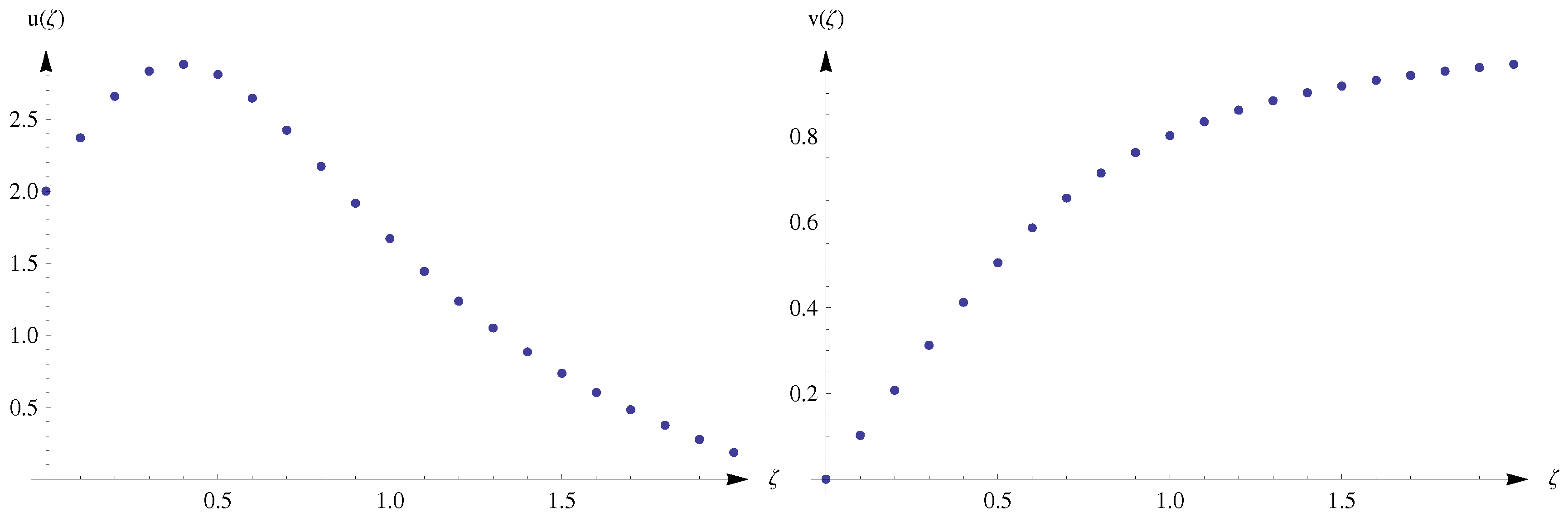
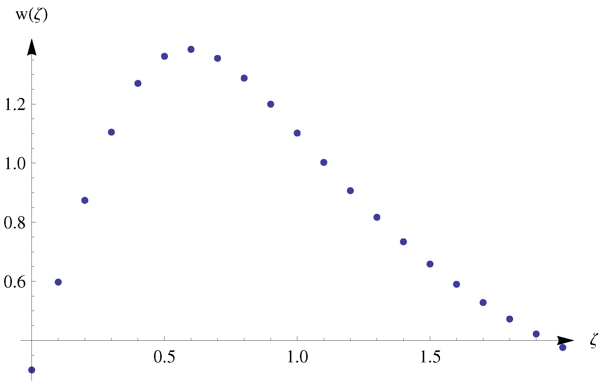
4. Numerical Solutions

According to (54) one has

$$\begin{array}{c}\hfill w^{\prime }=\zeta u^{\prime }.\end{array}$$

(74)

Substitute (74) into (57), one has

$$\begin{array}{c}\hfill (\nu +u-\zeta u^{\prime })w+{\zeta }^2(3\nu +u)u^{\prime }+\nu (1+{\zeta }^2)w^{″}-\frac{g^{\prime }}{\rho }=0.\end{array}$$

(75)

In order to solve the numerical solutions of the initial value problems in ODEs (55), (56),(75) and (72) by using the Runge-Kutta method, we considers $g\left(\zeta \right)=c_7+c_8\zeta$. Firstly, we change (55), (56), (75) and (72) into first order initial value problems in ODEs. Let

$$\begin{array}{c}{y}_1=u,y_2=u^{\prime },y_3=v,y_4=v^{\prime },y_5=w,y_6=w^{\prime },\hfill \end{array}$$

(76)

then Equations (55), (56) and (75) are changed into the following form

$$\begin{array}{c}{y}_1^{\prime }=y_2,y_2^{\prime }=-\frac{1}{\nu (1+{\zeta }^2)}[y_1^2+y_3^2+\frac{1}{\rho }(2c_7+3c_8\zeta )+(3\nu \zeta +\zeta y_1-y_5)y_2],\hfill \end{array}$$

(77)

$$\begin{array}{c}{y}_3^{\prime }=y_4,y_4^{\prime }=-\frac{1}{\nu (1+{\zeta }^2)}(3\nu \zeta +\zeta y_1-y_5)y_4,\hfill \end{array}$$

(78)

$$\begin{array}{c}{y}_5^{\prime }=y_6,y_6^{\prime }=-\frac{1}{\nu (1+{\zeta }^2)}[y_5(\nu +y_1-y_6)+\zeta (3\nu +y_1)y_6-\frac{c_8}{\rho }].\hfill \end{array}$$

(79)

The corresponding initial conditions have the following form

$$\begin{array}{c}\hfill y_1\left(0\right)=c_1,y_2\left(0\right)=c_2,y_3\left(0\right)=c_3,y_4\left(0\right)=c_4,y_5\left(0\right)=c_5,y_6\left(0\right)=c_6.\end{array}$$

(80)

We let

$$\begin{array}{c}{f}_1=y_2,f_2=-\frac{1}{\nu (1+{\zeta }^2)}[y_1^2+y_3^2+\frac{1}{\rho }(2c_7+3c_8\zeta )+(3\nu \zeta +\zeta y_1-y_5)y_2],\hfill \end{array}$$

(81)

$$\begin{array}{c}{f}_3=y_4,f_4=-\frac{1}{\nu (1+{\zeta }^2)}(3\nu \zeta +\zeta y_1-y_5)y_4,\hfill \end{array}$$

(82)

$$\begin{array}{c}{f}_5=y_6,f_6=-\frac{1}{\nu (1+{\zeta }^2)}[y_5(\nu +y_1-y_6)+\zeta (3\nu +y_1)y_6-\frac{c_8}{\rho }],\hfill \end{array}$$

(83)

where $f_1,f_2,f_3,f_4,f_5,f_6$ are the functions of $\zeta ,y_1,y_2,y_3,y_4,y_5,y_6$, then we give the following Runge-Kutta formula

$$\begin{array}{c}{y}_{i,n+1}=y_{in}+\frac{h}{6}(K_{i1}+2K_{i2}+2K_{i3}+K_{i4}),i=1,\cdots ,6.\hfill \\ K_{i1}=f_i({\zeta }_n,y_{1n},y_{2n},y_{3n},y_{4n},y_{5n},y_{6n})\hfill \\ K_{i2}=f_i({\zeta }_n+\frac{h}{2},y_{1n}+\frac{h}{2}{K}_{11},y_{2n}+\frac{h}{2}{K}_{21},y_{3n}+\frac{h}{2}{K}_{31},y_{4n}+\frac{h}{2}{K}_{41},y_{5n}+\frac{h}{2}{K}_{51},y_{6n}+\frac{h}{2}{K}_{61})\hfill \\ K_{i3}=f_i({\zeta }_n+\frac{h}{2},y_{1n}+\frac{h}{2}{K}_{12},y_{2n}+\frac{h}{2}{K}_{22},y_{3n}+\frac{h}{2}{K}_{32},y_{4n}+\frac{h}{2}{K}_{42},y_{5n}+\frac{h}{2}{K}_{52},y_{6n}+\frac{h}{2}{K}_{62})\hfill \\ K_{i4}=f_i({\zeta }_n+h,y_{1n}+h{K}_{13},y_{2n}+h{K}_{23},y_{3n}+h{K}_{33},y_{4n}+h{K}_{43},y_{5n}+h{K}_{53},y_{6n}+h{K}_{63})\hfill \end{array}$$

(84)

where ${\zeta }_0=0,{\zeta }_n={\zeta }_0+nh,$ and h is the step size.

Figure 1 and Figure 2 show the numerical solutions of $u\left(\zeta \right),v\left(\zeta \right),w\left(\zeta \right)$ in [0,2] when the parameters have the following proper values:

$$\begin{array}{c}\hfill c_1=2,c_2=4,c_3=0,c_4=1,c_5=0.3,c_6=3,c_7=0.1,c_8=0.2,\rho =100,\nu =0.6,h=0.1.\end{array}$$

(85)

5. Conclusions

In this paper, the application of the symmetry method on BVP for nonlinear PDEs is studied. Firstly, we have got the multi-parameter symmetry of von K$\acute{a}$rm$\acute{a}$n swirling viscous flow based on the differential characteristic set algorithm. Via twice symmetry reducions, BVP (11)–(18) became an initial value problem of ODEs. Secondly, we solved numerically the initial value problem of ODEs by using the Runge-Kutta method. The differential characteristic set algorithm is a key factor which influences the calculation of the symmetry of PDEs.

We considered that the boundary conditions are the arbitrary functions $B_i(r,\theta )$. However, $B_i(r,\theta )$ are determined by using the invariance of the boundary conditions under a multi-parameter Lie group of transformations. This approach is different from other research. For example, the boundary conditions are given by the following forms $V_r(r,\theta ,0)=0,V_z(r,\theta ,0)=0$ in [30]. The Lie symmetry and Runge-Kutta methods are effective methods which are applied to solving PDEs. Hence, their combination will advance the availability of solutions. At present, it is very valuable to solve nonlinear PDEs by combining the symmetry method, the differential characteristic set algorithm and other methods.

References

1. Lie, S. Vorlesungen uber Differentialgleichungen Mit Bekannten Infinitesimalen Transformationen; BG Teubner: Leipzig, Germany, 1891. [Google Scholar]
2. Bluman, G.W.; Kumei, S. Symmetries and Differential Equations; Springer: New York, NY, USA; Berlin, Germany, 1989. [Google Scholar]
3. Olver, P.J. Applications of Lie Groups to Differential Equations; Spinger: New York, NY, USA; Berlin, Germany, 1986. [Google Scholar]
4. Bluman, G.W.; Cheviakov, A.; Anco, S. Applications of Symmetry Methods to Partial Differential Equations; Springer: New York, NY, USA; Berlin, Germany, 2010. [Google Scholar]
5. Ibragimov, N.H.; Ibragimov, R.N. Applications of Lie Group Analysis to Mathematical Modelling in Natural Sciences. Math. Model. Nat. Phenom. 2012, 7, 52–65. [Google Scholar] [CrossRef]
6. Ibragimov, N.H. CRC Handbook of Lie Group Analysis of Differential Equations; CRC Press: Boca Raton, FL, USA, 1994; Volume 1. [Google Scholar]
7. Ibragimov, N.H. CRC Handbook of Lie Group Analysis of Differential Equations; CRC Press: Boca Raton, FL, USA, 1995; Volume 2. [Google Scholar]
8. Tiwari Ajey, K.; Pandey, S.N.; Senthilvelan, M.; Lakshmanan, M. Lie point symmetries classification of the mixed Lienard-type equation. Nonlinear Dyn. 2015, 82, 1953–1968. [Google Scholar] [CrossRef]
9. Davison, A.H.; Kara, A.H. Potential Symmetries and Associated Conservation Laws with Application to Wave Equations. Nonlinear Dyn. 2003, 33, 369–377. [Google Scholar] [CrossRef]
10. Chaolu, T.M.; Bai, Y.S. An Algorithm for Determining Approximate Symmetries of Differential Equations Based on Wu’s Method. Chin. J. Eng. Math. 2011, 28, 617–622. [Google Scholar]
11. Ma, W.X. K-symmetries and τ-symmetries of evolution equations and their Lie algebras. J. Phys. A Math. Gen. 1990, 23, 2707–2716. [Google Scholar] [CrossRef]
12. Ma, W.X. A soliton hierarchy associated with so(3,R). Appl. Math. Comput. 2013, 220, 117–122. [Google Scholar]
13. Bluman, G.W.; Chaolu, T.M. Conservation laws of nonlinear telegraph equations. J. Math. Anal. Appl. 2005, 310, 459–476. [Google Scholar] [CrossRef]
14. Anco, S.; Bluman, G.W.; Wolf, T. Invertible mappings of nonlinear PDEs to linear PDEs through admitted conservation laws. Acta Appl. Math. 2008, 101, 21–38. [Google Scholar] [CrossRef]
15. Abdulwahhab, M.A. Exact solutions and conservation laws of the system of two-dimensional viscous Burgers equations. Commun. Nonlinear Sci. Numer. Simul. 2016, 39, 283–299. [Google Scholar] [CrossRef]
16. Avdonina, E.D.; Ibragimov, N.H.; Khamitova, R. Exact solutions of gasdynamic equations obtained by the method of conservation laws. Commun. Nonlinear Sci. Numer. Simul. 2013, 18, 2359–2366. [Google Scholar] [CrossRef]
17. Ma, W.X. Conservation Laws of Discrete Evolution Equations by Symmetries and Adjoint Symmetries. Symmetry 2015, 7, 714–725. [Google Scholar] [CrossRef]
18. Wang, G.W.; Liu, X.Q.; Zhang, Y.Y. Symmetry reduction, exact solutions and conservation laws of a new fifth-order nonlinear integrable equation. Commun. Nonlinear Sci. Numer. Simul. 2013, 18, 2313–2320. [Google Scholar] [CrossRef]
19. Sahoo, S.; Saha Ray, S. Lie symmetry analysis and exact solutions of (3+1) dimensional Yu-Toda-Sasa- Fukuyama equation in mathematical physics. Comput. Math. Appl. 2017, 73, 253–260. [Google Scholar] [CrossRef]
20. Ma, W.X.; Chen, M. Direct search for exact solutions to the nonlinear Schrödinger equation. Appl. Math. Comput. 2009, 215, 2835–2842. [Google Scholar]
21. Yang, H.Z.; Liu, W.; Yang, B.Y.; He, B. Lie symmetry analysis and exact explicit solutions of three-dimensional Kudryashov-Sinelshchikov equation. Commun. Nonlinear Sci. Numer. Simul. 2015, 27, 271–280. [Google Scholar] [CrossRef]
22. Yang, S.J.; Hua, C.C. Lie symmetry reductions and exact solutions of a coupled KdV-Burgers equation. Appl. Math. Comput. 2014, 234, 579–583. [Google Scholar] [CrossRef]
23. Seshadri, R.; Na, T.Y. Group Invariance in Engineering Boundary Value Problems; Springer: New York, NY, USA; Berlin/Heidelberg, Germany; Tokyo, Japan, 1985. [Google Scholar]
24. Yürüsoy, M.; Pakdemirli, M.; Noyan, Ö.F. Lie group analysis of creeping flow of a second grade fluid. Int. J. Non-Linear Mech. 2001, 36, 955–960. [Google Scholar]
25. Vaneeva, O.O.; Papanicolaou, N.C.; Christou, M.A.; Sophocleous, C. Numerical solutions of boundary value problems for variable coefficient generalized KdV equations using Lie symmetries. Commun. Nonlinear Sci. Numer. Simul. 2014, 19, 3074–3085. [Google Scholar] [CrossRef]
26. Bilige, S.D.; Wang, X.M.; Morigen, W.Y. Application of the symmetry classification to the boundary value problem of nonlinear partial differential equations (in Chinese). Acta Phys. Sin. 2014, 63, 040201. [Google Scholar]
27. Gai, L.T.; Bilige, S.D.; Jie, Y.M. The exact solutions and approximate analytic solutions of (2+1)-dimensional KP equation based on symmetry method. SpringerPlus 2016, 5, 1267. [Google Scholar] [CrossRef] [PubMed]
28. Bilige, S.D.; Han, Y.Q. Symmetry reduction and numerical solution of a nonlinear boundary value problem in fluid mechanics. Int. J. Numer. Methods Heat Fluid Flow 2018, 28, 518–531. [Google Scholar] [CrossRef]
29. Chaolu, T.M.; Bai, Y.S. A new algorithmic theory for determining and classifying classical and non-classical symmetries of partial differential equations (in Chinese). Sci. China Math. 2010, 40, 331–348. [Google Scholar]
30. Yang, C.; Liao, S.J. On the explicit, purely analytic solution of Von Kármán swirling viscous flow. Commun. Nonlinear Sci. Numer. Simul. 2006, 11, 83–93. [Google Scholar] [CrossRef]
Figure 1. Numerical solutions of u ( ζ ) , v ( ζ ) in [0,2].
Symmetry 10 00120 g001
Figure 2. Numerical solutions of w ( ζ ) in [0,2].
Symmetry 10 00120 g002