Research on Electronic Voltage Transformer for Big Data Background


1
China Three Gorges University College of Electrical Engineering & New Energy, Yichang 443002, China
2
Hubei Provincial Collaborative Innovation Center for New Energy Microgrid, China Three Gorges University, Yichang 443002, China
3
School of Electronic and Information Engineering, Suzhou University of Science and Technology, Suzhou 215009, China
*
Author to whom correspondence should be addressed.
Symmetry 2018, 10(7), 234; https://doi.org/10.3390/sym10070234
Submission received: 27 May 2018
/
Revised: 13 June 2018
/
Accepted: 17 June 2018
/
Published: 21 June 2018
(This article belongs to the Special Issue Emerging Approaches and Advances in Big Data)
Abstract
:A new type of electronic voltage transformer is proposed in this study for big data background. By using the conventional inverted SF_6 transformer insulation structure, a coaxial capacitor sensor was constructed by designing a middle coaxial electrode between the high-voltage electrode and the ground electrode. The measurement of the voltage signal could be obtained by detecting the capacitance current i of the SF_6 coaxial capacitor. To improve the accuracy of the integrator, a high-precision digital integrator based on the Romberg algorithm is proposed in this study. This can not only guarantee the accuracy of computation, but also reduce the consumption time; in addition, the sampling point can be reused. By adopting the double shielding effect of the high-voltage shell and the grounding metal shield, the ability and stability of the coaxial capacitor divide could be effectively improved to resist the interference of stray electric fields. The factors that affect the coaxial capacitor were studied, such as position, temperature, and pressure, which will influence the value of the coaxial capacitor. Tests were carried out to verify the performance. The results showed that the voltage transformer based on the SF_6 coaxial capacitor satisfies the requirements of the 0.2 accuracy class. This study can promote the use of new high-performance products for data transmission in the era of big data and specific test analyses.
1. Introduction
The development of the smart grid has reached consensus around the world [1,2,3]. The smart grid has the characteristics of covering a wide range of geographical locations, controlling a large amount of energy transmission, and regulating the real-time balance of power transmission. These characteristics make the power grid generate a huge amount of data at run time, which provide a foundation for using big data technology. With the development of the Internet, the application of big data technology is becoming more and more extensive. The important feature of big data is that it requires the timely collection of a large number of rapidly changing parameters of power systems, characterized by high speed, big scale, and diversity. In order to ensure the safe and stable operation of the power grid, it is necessary to control the running state of the power grid in real time and obtain a large amount of instantaneous data as the data source of the big data technology [4,5]. As an important measuring equipment of an electrical circuit, the electronic transformer is suitable for the demand of this era with its unique advantages of low power consumption, low consumable material, fast response speed, wide dynamic range, and capability of remote transmission [6].
The research on electronic transformers started in the 1960s, and many companies engaged in correlative research. Countries such as the US, Japan, and France have studied prototypes and operated separately [7]. In China, Xi’an Jiao Tong University, Huazhong University of Science and Technology, and other universities and institutes are also carrying out related research and producing many products, such as an optoelectronic effect electronic voltage transformer studied by Huazhong University of Science and Technology, which was operated in a 110 kV substation in Guangdong power grid [8].
Although great progress has been made for the electronic voltage transformer, there are still problems to solve. For optical voltage transformers, the performance is unstable and easily affected by temperature variations, while the voltage transformer based on series of multiple capacitance is susceptible to the external stray capacitance, and its performance is not stable [9,10].
To solve these problems, an electronic voltage transformer based on a coaxial capacitor and digital integration is proposed in this study. The unique overall structure of the electronic voltage transformer has the advantages of a strong ability to resist external stray electric field interference, a high measurement accuracy, and a good stability. To improve the accuracy of the integrator, a new integration algorithm was developed to reduce the computation time and improve the accuracy. The results show that the electronic voltage transformer can meet the accuracy requirements of 0.2 level in IEC60044-7 and GBT 20840.7-2007 and has a very prominent application and industrialization prospect.
2. Principle and Structure
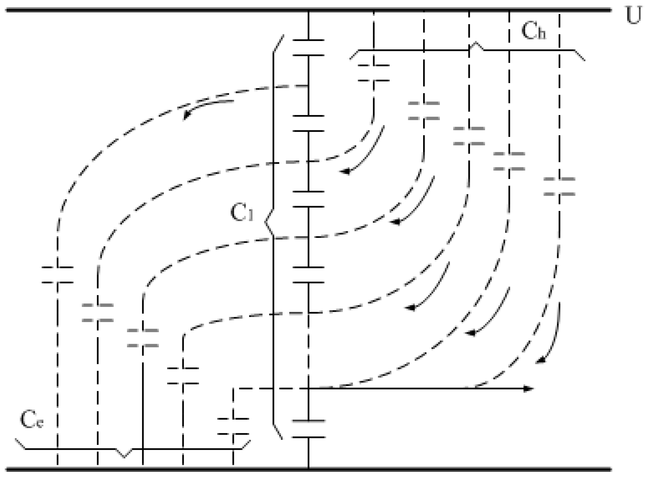
The research on high-voltage transformers is mainly focusing on two aspects. One is the series of multiple-capacitance voltage transformer and the other is the optical voltage transformer [11]. The temperature stability of the optical voltage transformer is poor, and the measurement accuracy may be affected. The manufacturing process requirements are numerous and lead to a higher cost [12]. For the voltage transformer based on series of multiple capacitance transformers, although the ferromagnetic resonance existing in the traditional CVT (Capacitor Voltage Transformer) is eliminated, the equivalent capacitance of the series high-voltage capacitor is sensitive to the parasitic capacitance for the high-voltage side Ch and the parasitic capacitance Ce to the ground. Figure 1 is a schematic of the distribution of Ch and Ce. Ch is usually smaller than Ce, and the combination of the two capacitances is equivalent to a smaller parasitic capacitance to the ground, which is usually called the equivalent parasitic capacitance Ced to the ground. Part of the current will flow through the parasitic capacitance Ce to the ground because of the existence of Ced, which will cause a change in measurement accuracy and make the anti-electromagnetic interference poor. Although the increase of the capacitance can reduce this effect, the price and size will increase sharply [13].
In order to solve the above problems, the electronic voltage transformer proposed in this study combines the insulation technology of the traditional inverted SF_6 transformer and the new sensing technology. The voltage sensor uses the SF_6 coaxial capacitor as the high voltage capacitor to construct the voltage sensor, which eliminates the inherent ferromagnetic resonance of traditional voltage transformers. The high-voltage shell and the grounding metal shield play a double shielding function. They can effectively eliminate the influence of the parasitic capacitance and have good electromagnetic interference resistance and high stability.
The structure of the proposed voltage transformer is shown in Figure 2. Each part is explained in detail in Figure 2. It can be seen from the figure that it mainly consists of three parts: the high-voltage shell, the insulating sleeve, and the grounding system. The high-voltage shell part consists of an explosion-proof slice, a high-voltage shell, a primary connection terminal, a primary conductor, a metal shield, and a capacitor ring. The capacitor ring is installed in the inner side of the metal shield. The insulating sleeve part consists of an insulating sleeve and a metal tube. The grounding system part consists of a gas density meter, a grounding guide rod, a base, a secondary connection boxes, and a nameplate. The interior of the high-voltage shell and the insulating sleeve are insulated by SF_6 gas. The primary connection terminal is connected to high-voltage, so the high-voltage shell and the primary conductor are on the high-potential side. The metal shield is connected to the earthing screw through the metal tube, so it is on the low-potential side. The insulation between the high-voltage and low-voltage potentials is obtained with SF_6 gas.
The structure of the SF_6 coaxial capacitor is shown in Figure 3. It consists of a metal shield, a capacitor ring, a primary conductor, a high-voltage shell, a ground electrode, and an insulating layer. A capacitor ring is installed between the primary conductor and the metal shield. The principle of measuring high voltage by using the SF_6 coaxial capacitor is as follows: The primary conductor 3 is connected to the high-voltage side. The high-voltage shell 4 and the primary conductor 3 are at high potential and used as a high-voltage electrode. The metal shield 1 is at the ground potential and used as a low-voltage electrode. The capacitor ring 2 is installed at the inside of 1 (1 and 2 are insulated by the insulating layer 6). The diameter of the capacitor ring is 300 mm, and its width is 50 mm. The capacitor ring 2 is between the high- and low-voltage electrodes and is insulated from them to form a middle electrode. The capacitor ring and the high- and low-voltage electrodes produce two capacitors. Capacitance C1 of the high-voltage side is formed by the capacitor ring and the primary conductor. Its output is transmitted to the low-voltage side by a shield cable. Its value can be given as:
where
D1 is the diameter of the capacitor ring (m).
D2 is the diameter of the primary conductor (m).
l is the width of the capacitor ring (m).
is the permittivity of vacuum.
is the relative permittivity of the SF_6 gas.
The voltage of the high-voltage side can be obtained by detecting the current i in the capacitor. The capacitance current i is proportional to the primary voltage u, the angular frequency ω, and the value of the C1.
The capacitance current is a differential signal of the primary voltage. Therefore, it is necessary to integrate the capacitance current to eliminate the influence of frequency fluctuation.
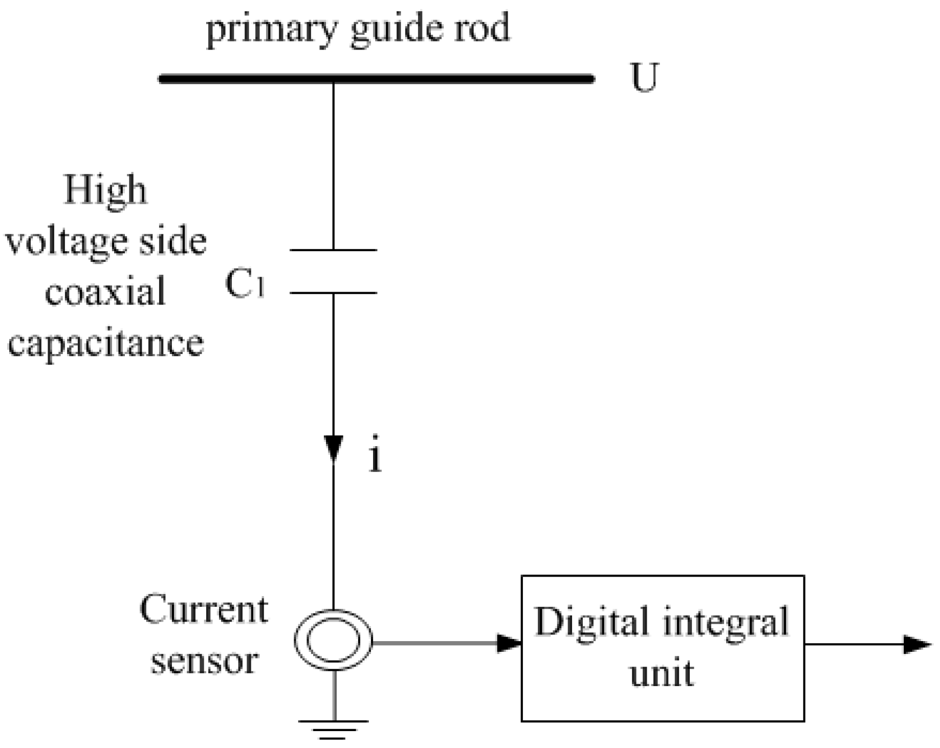
As shown in the Figure 4, the current signal of the SF_6 coaxial capacitor connects to the digital integration unit after the transformation of the current sensor. The digital integration unit is used to restore the current of the SF_6 coaxial capacitor to a signal which is proportional to the primary voltage. It is realized by the digital integrator in this study, which is not affected by temperature and other factors and greatly improves the accuracy and reliability of the integral link. The following is the design of the digital integration.
3. High-Precision Digital Integrator
The Romberg algorithm has the characteristics of high algebraic accuracy and fast convergence speed. It can improve the accuracy without increasing the computation as an extrapolation algorithm. It is well-suited to the needs of the big data age. The Romberg algorithm is used to achieve high-precision digital integrators. The principle is as follows: The error between the approximate integral value obtained by the trapezoidal formula and the exact value is about . The error is used as a compensation for , and the result is exactly the approximate value obtained by the Simpson formula. According to the conclusion, the Romberg algorithm is summed as shown in Formula (3) [14], in which, n represents the multiple of the sampling frequency, 1 represents the sampling frequency when it is doubled, 0 represents the sampling frequency when it is a constant, and −1 represents the sampling frequency when it is halved. The basic principle of the Romberg algorithm is shown in Figure 5.
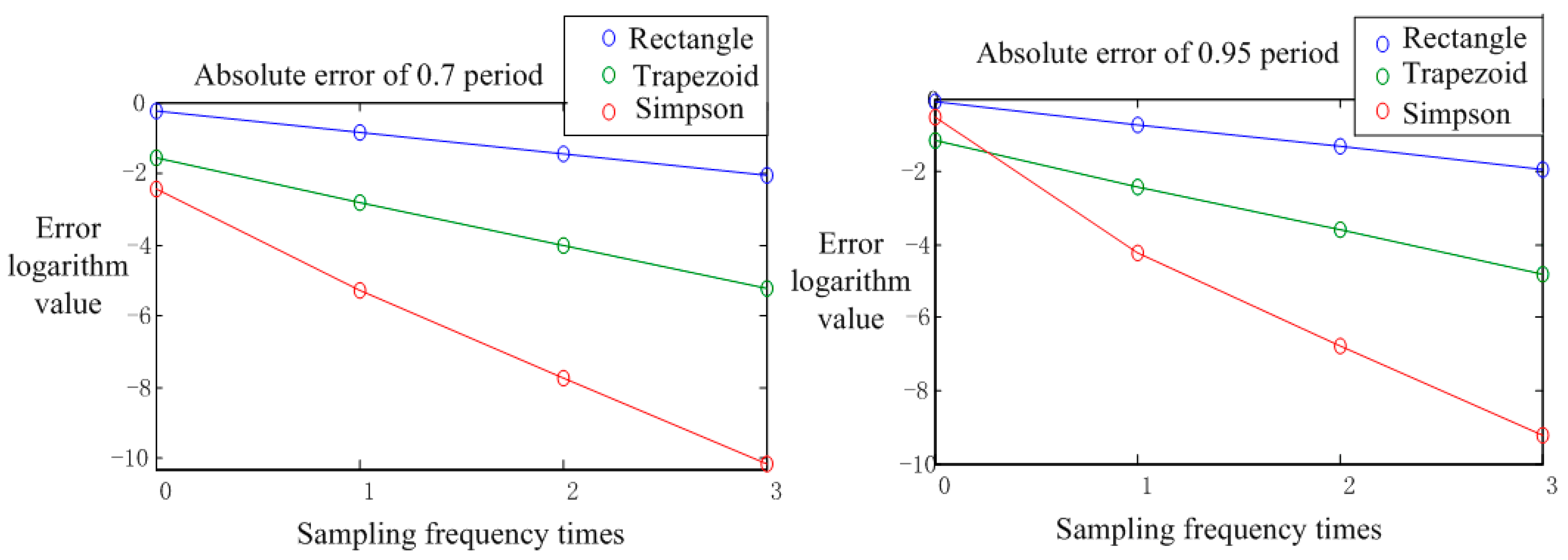
According to the definition of the Newton Cotes algorithm, the complex trapezoid, complex rectangle, and complex Simpson formula can be obtained as follows. The logarithm λ of the error is introduced for the convenience of comparison, and the error logarithm formula is defined as the Formula (7):
Simulating the amplitude error of the Formulas (4)–(6) and then combining the Formula (7), the results can be obtained as shown in Figure 6. Finally, the following conclusions can be drawn from Figure 6:
- (1)
- Improving the sampling frequency has obvious effects on improving the amplitude characteristic of the digital integrator.
- (2)
- The complex Simpson formula is more accurate than the complex trapezoidal formula, and the error is reduced faster [15].
Because of the limited resolution of the analog–digital converter, the sampling frequency of the electronic current transformer in the actual work cannot be unrestrictedly increasing. In addition, integrating the requirement of sampling points and calculation speed, as well as cost performance, it is not advisable to improve the digital integrator only by increasing the sampling frequency.
Using the Romberg algorithm and combining the method that increases the sampling frequency to reduce the error, it can be concluded that the effect of improving the error by increasing the sampling frequency is further improved with the improvement of the orders of the transfer function in the Coates algorithm. A complex Simpson transfer function is obtained by linearly combining the complex trapezoid formula. The three-order formula is obtained by linear combination of the Simpson transfer function. Followed by analogy according to Formula (7), we can find that the new logarithmic function transfer error is linearly decreased when constructed by the Romberg algorithm. In this way, a new transfer function can be constructed according to the magnitude of the minimum acceptable error [16].
As for the sampling delay that produces non-integer, it is constructed by the traditional cascade filter. The specific transfer function can be designed and implemented in DSP (Digital Signal Processing) or FPGA (Field-Programmable Gate Array). The disadvantages of using these methods are: even if using the simplest trapezium formula to make a linear combination before and after two points of step length, the form of the transfer function obtained after three successive combinations is also very complex, which leads to the rapid increase of the number of sampling points needed and to the reduction of the computing speed. In the same way, its design form is more complex.
The algorithm with higher order is more accurate and faster with the increase of the sampling frequency. However, in practical application, the high-order formula should be avoided as much as possible because of the limitations of the stability and the number of sampling points. A split method to reversely decompose the transfer function is proposed in this study by using the Romberg algorithm. The high-precision and complicated transfer function is reversely decomposed into two or more transfer functions, such as in Formula (8). From Figure 6, it can be observed that the error of the transfer function is about 10−4, and the precision is high in the 0.95π. At the same time, the form of Formula (8) is simple and easy to design, and the phase is −90 degree in the whole frequency band, so the error of the phase characteristic is unnecessary to consider.
Owing to the computer-calculated integral value with interval successive half way to calculate, a previous segmentation function integral value after the integral interval divided into half can also be used. So, a dual microprocessor is chosen to synchronize the work. A simple transfer function is implemented in each microprocessor, which cannot only guarantee the accuracy of computation, but also overcome the difficulty of design and achieve the reduction of consumption time, and the sampling point can also be reused.
The structure of a dual-channel digital integrator is designed in this study on the basis of the Romberg algorithm, which has high precision and simple design. The structure is shown in Figure 7.
The differential signal output by the coaxial capacitor is first amplified by an active amplifier, and the DC component interference is eliminated after high-pass filtering; then, the signal enters the parallel-channel processing structure. The parallel-channel processing structure includes two channels. The ADC sampling frequency in the main channel is set to f, and the sampling frequency in the error compensation channel is 0.5f. That is, the sampling frequency in the error compensation channel is reduced to half that of the main channel. The signal is sent to the digital integral link after the analog-to-digital converter to carry out the digital integral processing. The transfer function of the digital integral link can be designed as two complex trapezoid transfer functions (9) and (10) according to Formula (8).
The digital integration unit and the proportional link use the microprocessor as the hardware implementation platform. The output of the digital integration unit is adjusted by the proportion adjustment, and the result is output after adding in the adder, which is provided for the use of the follow-up equipment.
The Romberg algorithm applied to the high-order transfer function only needs to change the corresponding proportional link coefficient and design the integral transfer function. Therefore, the structure is universal.
The errors of the complex rectangular, trapezoid, and Simpson transfer functions are given in Table 1, according to Formula (11). We can see that the error in the 0.95π period is 4.0266 × 10⁻³ using Formula (10) to construct a traditional digital integrator, and the error is reduced to 5.7389 × 10⁻⁵ after the error compensation channel is added on the basis of Figure 7. The results of Table 1 show that the dual -hannel digital integrator has the characteristics of simple design and high accuracy. Meanwhile, the program design of the integral link can also be reduced, which can improve the computation speed and reduce the computation time.
4. Performance Analysis
Changes of the capacitance will affect the accuracy of the voltage measurement as the coaxial capacitor will change with the position, temperature, and pressure. The coaxial capacitor is related to the dielectric constant of the medium when the structure of the coaxial capacitor is determined. The SF_6 gas, with excellent insulation and arc extinguishing properties, is used in the medium [17]. The detailed analysis is as follows.
4.1. Analysis of Position Influence of the SF_6 Coaxial Capacitor
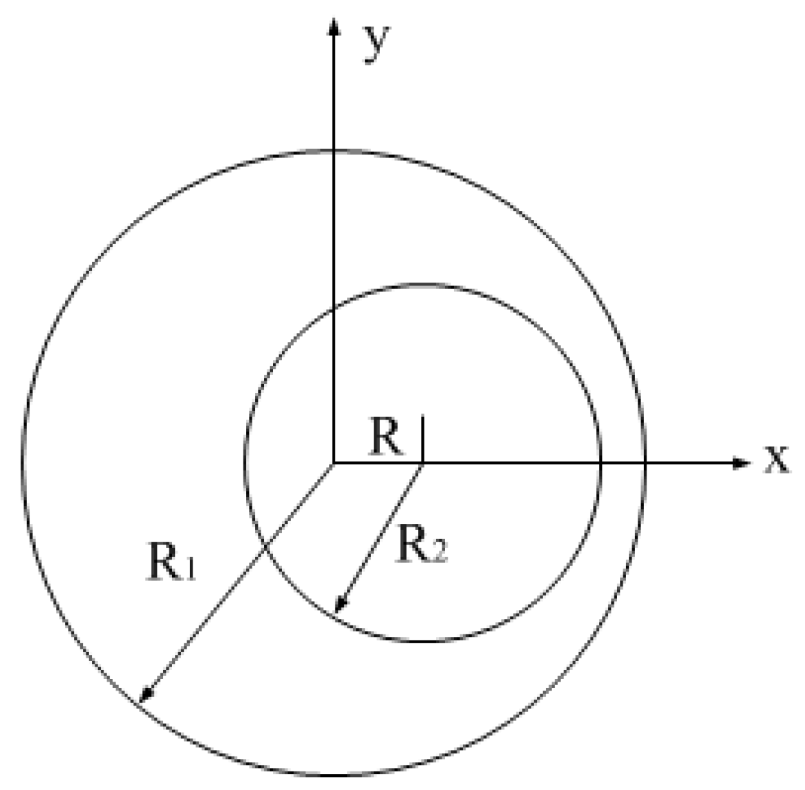
The inner and outer radii of the two coaxial cylindrical conductor shells are R1 and R2, and R2 > R1. The length of the cylinder is l. Suppose l >> (R2 − R1), the capacitance between the two cylindrical conductor shells can be obtained:
4.1.1. Calculation of Off-Axis Capacitance
As shown in Figure 8, on the basis of Formula (12), the capacitance can be obtained when the cylindrical conductor shells is off-axis.
where
R is the distance between the inner and outer centers of the circle.
is the length of the conductor shell.
4.1.2. Calculation of the Deflection Angle Capacitance
When off-center, the capacitance of each unit length varies with the distance between the two circular centers; taking two limit conditions as follows:
When R = 0:
When R = R2 − R1:
It can be seen from the above deduction that the capacitance is the smallest when the centers of the circles coincide, and the capacitance is maximum when the two circles are internally tangent, which is the case of the bias axis. When the angle is deflected, it can divide the cable infinitely in the direction perpendicular to the axis of the cable. Each section can be equivalent to a very small axis of bias, then the capacitance, in the case of deflection, is integral along the inner axis. Because of the inverse correlation between C and R, the influence of the drift angle should be less than that of the bias axis, so the effect of the deflection angle can be ignored in practice.
4.1.3. Off-Axis Distance Allowed in Practice
The error of the 0.2 class electronic voltage transformers must not exceed 0.2% according to the IEC standards. The precision of the primary voltage sensor should be controlled within 0.05% according to the principle of error distribution. Because the output of the primary voltage sensor is proportional to the SF_6 coaxial capacitor, the capacitance change caused by the off-axis should be less than 0.05%. For the designed transformer, R1 = 45 mm and R2 = 135 mm. The simulation results are shown in Figure 9.
From Figure 9 it can be seen that the error is within the allowable error range when the off-axis distance is 2.5 mm.
4.2. Analysis of Temperature Performance and Pressure Performance of the Coaxial Capacitor
When the pressure of the SF_6 gas P is from 0.3 to 2.0 MPa, and the temperature T is from 250 to 600 K, the density can be calculated according to the Beattie–Bridgman formula [18].
where:
P is the pressure (MPa).
T is the temperature (K).
ρ is the density (Kg/m3).
The changes of can be calculated by Formula (18).
The relationship among the gas molecular density N in Formula (18) and the pressure and temperature can be expressed as in Formula (19).
where, k is the Boltzmann constant with the value of 1.38 × 10⁻²³ J/K.
Substituting the Formula (19) into (18), the relative permittivity of the SF_6 gas can be obtained [19].
where and are all constants. Therefore, the relative permittivity increases with the increases of pressure in a certain range, and decreases with the increases of temperature.
4.2.1. The Relationship between the Capacitance and the Temperature When the Density Does Not Change
When the ambient temperature is 25 °C and the gas pressure is 0.1 MPa, the density of the SF_6 gas is 6.14 kg/m3. The relationship between P and T can be obtained by Formula (21).
The coaxial capacitance is:
where
is the molecular radius of the SF_6 gas, .
l is the length of the coaxial capacitor ring.
R1 and R2 are the inner and outer radii.
is the permittivity of vacuum.
Substituting (21) into (22), we obtain:
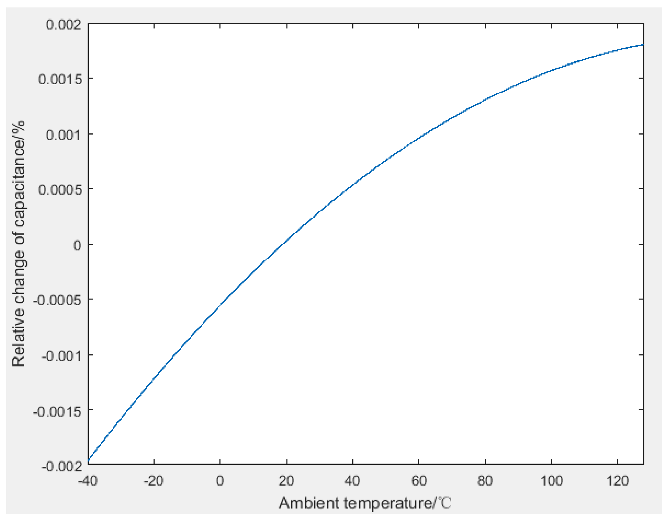
where the unit of the capacitance in the Formula (23) is pF. The relationship between C (pF) and T (°C) is shown in Figure 10.
As can be seen from Figure 10, the variation of the capacitance is less than 0.01% in the range of −40 to 120 °C, which meets the accuracy requirements of the 0.2 accuracy class.
4.2.2. The Relationship between the Capacitance and the Temperature When the Density Changes
In general, the annual leakage rate of the gas is less than 1%. Considering the worst case and assuming that the density of the SF_6 gas is changed to 99% of the initial value because of the leakage:
Substituting (24) into (23), we can obtain:
As can be seen from Figure 11, the change of the capacitance is less than 0.01% when the temperature changes in the range of −40 to 120 °C.
The results show that the designed SF_6 coaxial capacitor meets the precision requirements of the 0.2 accuracy class.
5. Experimental Results and Analysis
According to the accuracy requirements in IEC standards and GBT 20840.7-2007 [20,21,22], the experiments on the accuracy, power frequency, partial discharge, and electromagnetic compatibility of the developed transformer were completed at the National Power Grid Corp, Wuhan High-Voltage Research Institute. The basic accuracy test was carried out by comparison with a high-accuracy standard voltage transformer in the 0.02 accuracy class, and the temperature cycle test was also done in a similar way, by controlling the temperature in a closed room. The rated primary voltage of the transformer was 110 kV, and the rated secondary output was a digital value of 2D41H. The test results were as follows:
5.1. Basic Accuracy Test
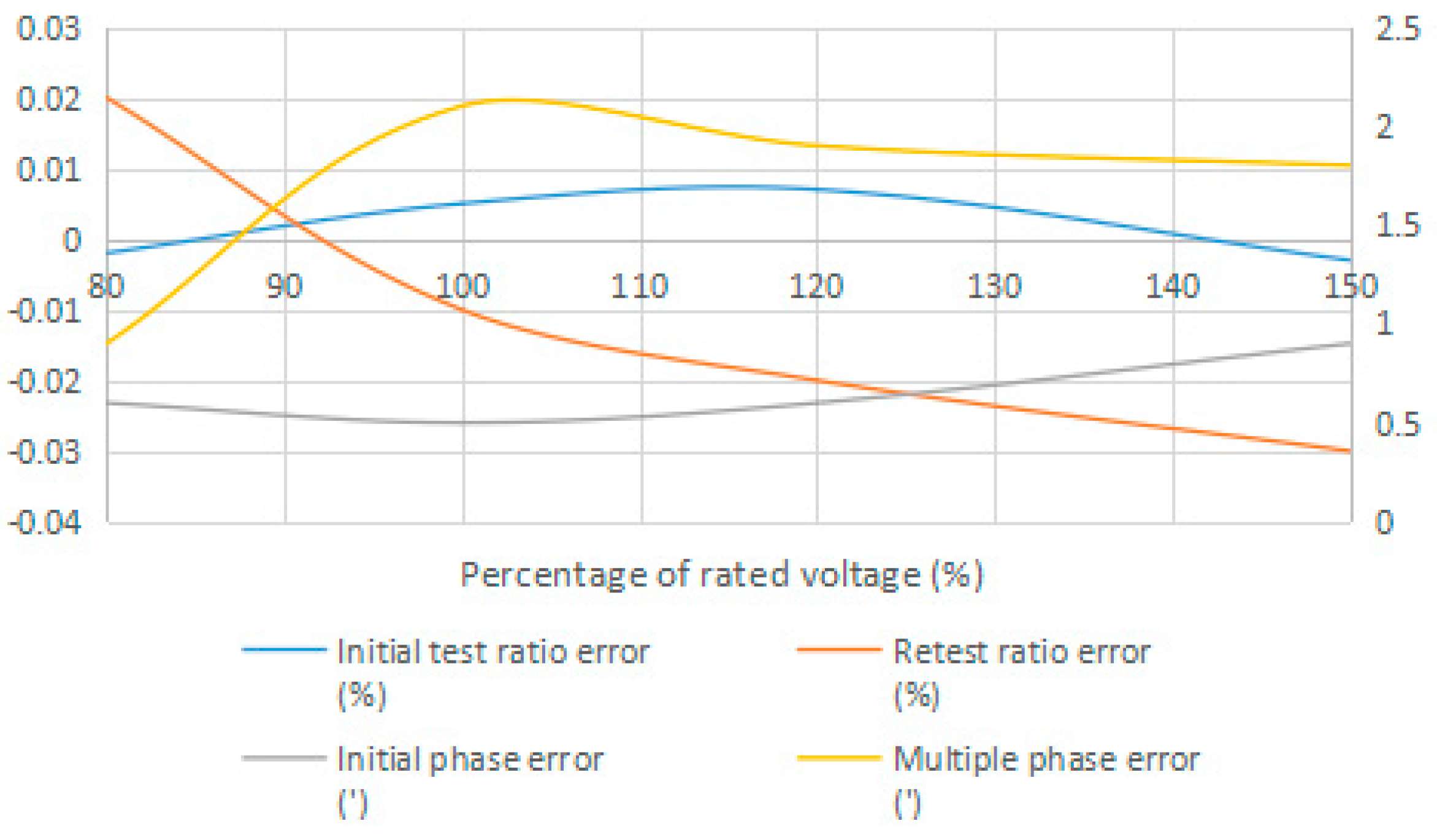
From the experimental results in Figure 12, we can see that the proposed electronic voltage transformer satisfied the accuracy requirements of the 0.2 class in the range of 80% to 150% of rated voltage. The variation of the ratio error was less than 0.05%, and the variation of the phase error was less than 2’. For the same test point, the difference of the initial ratio error and the retest value was less than 0.03%, and was 2’ for the phase.
5.2. Partial Discharge Test
The results in Table 2 showed that the partial discharge of the designed electronic voltage transformer met the requirements of the electronic voltage transformer in the standards.
5.3. EMC (Electromagnetic Compatibility) Test
According to the accuracy requirements in IEC standards and GBT 20840.7-2007, the electromagnetic field disturbance tests, surge immunity test, and oscillatory immunity test of the designed electronic voltage transformer were carried out. The results are shown in Table 3.
The results show that all the electromagnetic compatibility test items of the transformer reached grade A and fully met the requirements for outdoor operation.
5.4. Temperature Cycle Test
According to the requirements of the standards, the temperature cycle test of the designed electronic voltage transformer was carried out at the rated voltage. The results are shown in Figure 13.
The results show that the designed electronic voltage transformer met the accuracy requirements of the 0.2 class.
6. Conclusions
A new high-voltage electronic voltage transformer is proposed in this study, which meets the requirement of big data technology. By adopting the traditional inverted SF_6 insulation structure, a high reliability could be realized in the field operation. By constructing the middle coaxial electrode between the high-voltage electrode and the ground electrode, an SF_6 coaxial capacitor was formed, and the primary voltage could be obtained by detecting the current of the SF_6 coaxial capacitor. The capacitor was under the dual shielding of the high-voltage shell and the grounding metal shield, which could improve its stability. Factors affecting the coaxial capacitor were studied, such as position, temperature, and pressure, and the results showed that the transformer could achieve high accuracy and stability. To improve the performance of the integrator, a high-precision digital integrator based on the Romberg algorithm is proposed in this paper. This can not only guarantee the accuracy of computation, but also reduce the consumption time. In addition, the sampling point can also be reused. The test results showed that the electronic voltage transformer can fully meet the requirements of the 0.2 accuracy class.
Author Contributions
Z.-H.L. provided the main idea for this paper, designed the overall architecture of the proposed transformer, and wrote the paper. Y.W., Z.-T.W., and Z.-X.L. conducted the test data collection and designed the experiments.
Funding
This work was supported by China Scholarship Council and National Natural Science Foundation of China (Grant Number 51507091 and 61503270), National Science Foundation of Jiangsu Province (Grant Number BK20150326), National Science Found for Colleges and Universities of Jiangsu Province (Grant Number 15KJB510029), China Postdoctoral Science Foundation (Grant Number 2016M590497), and Jiangsu Provincial Department of Housing and Urban-Rural Development (Grant Number 2017ZD253).
Conflicts of Interest
The authors declare no conflict of interest.
Nomenclature
| Ch | parasitic capacitance for the high-voltage side (F); |
| Ce | parasitic capacitance to the ground (F); |
| Ced | equivalent parasitic capacitance to the ground (F); |
| C1 | capacitance C1 of the high-voltage side (F); |
| ε0 | permittivity of vacuum (8.85 × 10⁻¹² F/m); |
| l | width of the capacitor ring (m); |
| D1 | diameter of the the capacitor ring (m); |
| D2 | diameter of the primary conductor (m); |
| i | capacitance current (A); |
| u | primary voltage (V); |
| R1 | inner radius of the coaxial cylindrical conductor shells (m); |
| R2 | outer radius of the coaxial cylindrical conductor shells(m); |
| P | pressure (MPa); |
| T | temperature (K); |
| ρ | density (Kg/m3); |
| k | Boltzmann constant (1.38 × 10⁻²³ J/K); |
| molecular radius of the SF_6 gas (2.27 × 10⁻¹⁰ m). |
References
- Refaat, S.S.; Abu-Rub, H. Smart grid condition assessment: concepts, benefits, and developments. Power Electron. Drives 2016, 1, 147–163. [Google Scholar]
- Turner, M.; Liao, Y.; Du, Y. Comprehensive Smart Grid Planning in a Regulated Utility Environment. Int. J. Emerg. Electr. Power Syst. 2015, 16, 265–279. [Google Scholar] [CrossRef]
- Tu, C.; He, X.; Shuai, Z.; Jiang, F. Big data issues in smart grid—A review. Renew. Sustain. Energy Rev. 2017, 79, 1099–1107. [Google Scholar] [CrossRef]
- Munshi, A.A.; Yasser, A.-R.M. Big data framework for analytics in smart grids. Electr. Power Syst. Res. 2017, 151, 369–380. [Google Scholar] [CrossRef]
- Kovacevic, U.; Bajramovic, Z.; Jovanovic, B.; Lazarević, D.; Djekić, S. The construction of capacitive voltage divide for measuring ultrafast pulse voltage. In Proceedings of the IEEE Pulsed Power Conference (PPC), Austin, TX, USA, 31 May–4 June 2015; pp. 1–5. [Google Scholar]
- Li, N.; Zhang, J.; Chai, Z.; Wang, J.; Yang, B. The Application of Voltage Transformer Simulator in Electrical Test Training. In Proceedings of the IOP Conference Series: Earth and Environmental Science, Harbin, China, 8–10 December 2017; Volume 113. [Google Scholar]
- Xiang, L.; Bei, H.; Yue, T.; Tian, Y.; Fan, Y. Characteristic study of electronic voltage transformers’ accuracy on harmonics. In Proceedings of the China International Conference on Electricity Distribution (CICED), Xi’an, China, 10–13 August 2016; pp. 1–6. [Google Scholar]
- Morawiec, M.; Lewicki, A. Power electronic transformer based on cascaded H-bridge converter. Bull. Pol. Acad. Sci. Tech. Sci. 2017, 65, 675–683. [Google Scholar] [CrossRef] [Green Version]
- Santos, J.C.; de Sillos, A.C.; Nascimento, C.G.S. On-field instrument transformers calibration using optical current and voltage transformes. In Proceedings of the IEEE International Workshop on Applied Measurements for Power Systems Proceedings (AMPS), Aachen, Germany, 24–26 September 2014; pp. 1–5. [Google Scholar]
- Chen, X.S.; Li, Y.S.; Jiao, Y.; Lei, G.C. Distributed Capacitance Calculation Model in GIS Voltage Transformer’s Error Test. Appl. Mech. Mater. 2015, 378, 820–825. [Google Scholar] [CrossRef]
- Zhao, S.; Huang, Q.; Lei, M. Compact system for onsite calibration of 1000 kV voltage transformers. IET Sci. Meas. Technol. 2018, 12, 368–374. [Google Scholar] [CrossRef]
- Lebedev, V.D.; Yablokov, A.A. Studies in electromagnetic compatibility of optical and digital current and voltage transformers. In Proceedings of the IOP Conference Series: Materials Science and Engineering, Tomsk, Russia, 27–29 October 2016; Volume 177. [Google Scholar]
- Yin, X.D.; Jiang, C.Y.; Lei, M.; Xia, S.G.; Zhou, F. Research of Influence of Negative Voltage at Capacitance of Pulse Transformer of Pulse Power Generator. Appl. Mech. Mater. 2013, 2560, 1510–1514. [Google Scholar] [CrossRef]
- Frikha, N.; Huang, L. A multi-step Richardson-Romberg extrapolation method for stochastic approximation. Stoch. Process. Their Appl. 2015, 125, 4066–4101. [Google Scholar] [CrossRef]
- Polla, G. Comparison of Approximation Accuracy and time Integral Process between Simpson Adaptive Method and Romberg Method. J. Interdiscip. Math. 2015, 18, 459–470. [Google Scholar] [CrossRef]
- Li, Z.H.; Hu, W.Z. A high-precision digital integrator based on the Romberg algorithm. Rev. Sci. Instrum. 2017, 88, 045111. [Google Scholar] [CrossRef] [PubMed]
- Glushkov, D.A.; Khalyasmaa, A.I.; Dmitriev, S.A.; Kokin, S.E. Electrical Strength Analysis of SF6 Gas Circuit Breaker Element. AASRI Procedia 2014, 7, 57–61. [Google Scholar] [CrossRef]
- Lee, J.-C. Numerical Study of SF6 Thermal Plasmas Inside a Puffer-assisted Self-blast Chamber. Phys. Procedia 2012, 32, 822–830. [Google Scholar] [CrossRef]
- Ren, M.; Zhou, J.R.; Yang, S.J.; Zhuang, T.X.; Dong, M.; Albarracín, R. Optical Partial Discharge Diagnosis in SF6 gas-Insulated System with SiPM-based Sensor Array. IEEE Sens. J. 2018, 18, 5532–5540. [Google Scholar] [CrossRef]
- IEC 60044-7. Instrument Transformers Part 7: Electronic Voltage Transformers. Available online: https://webstore.iec.ch/publication/156 (accessed on 17 December 1999).
- IEC 61869-6. Instrument Transformers Part 6: Additional General Requirements for Low-Power Instrument Transformers. Available online: https://webstore.iec.ch/publication/24662 (accessed on 27 April 2016).
- GBT 20840.7-2007. Instrument Transformers Part 7: Electronic Voltage Transformers. Available online: http://www.anystandards.com/gbt/elec/20130221/22955.html (accessed on 16 January 2007).
Figure 1.
Schematic sketch of the distribution of the parasitic capacitance for the high-voltage side (Ch) and the parasitic capacitance to the ground (Ce).
Figure 1.
Schematic sketch of the distribution of the parasitic capacitance for the high-voltage side (Ch) and the parasitic capacitance to the ground (Ce).

Figure 2.
Basic structure of the SF_6 gas-insulated transformer. 1, explosion-proof slice; 2, high-voltage shell; 3, primary connection terminal; 4, insulating sleeve; 5, gas density meter; 6, primary conductor; 7, grounding guide rod; 8, base; 9, metal shield; 10, metal tube; 11, capacitor ring; 12, secondary connection boxes; 13, nameplate.
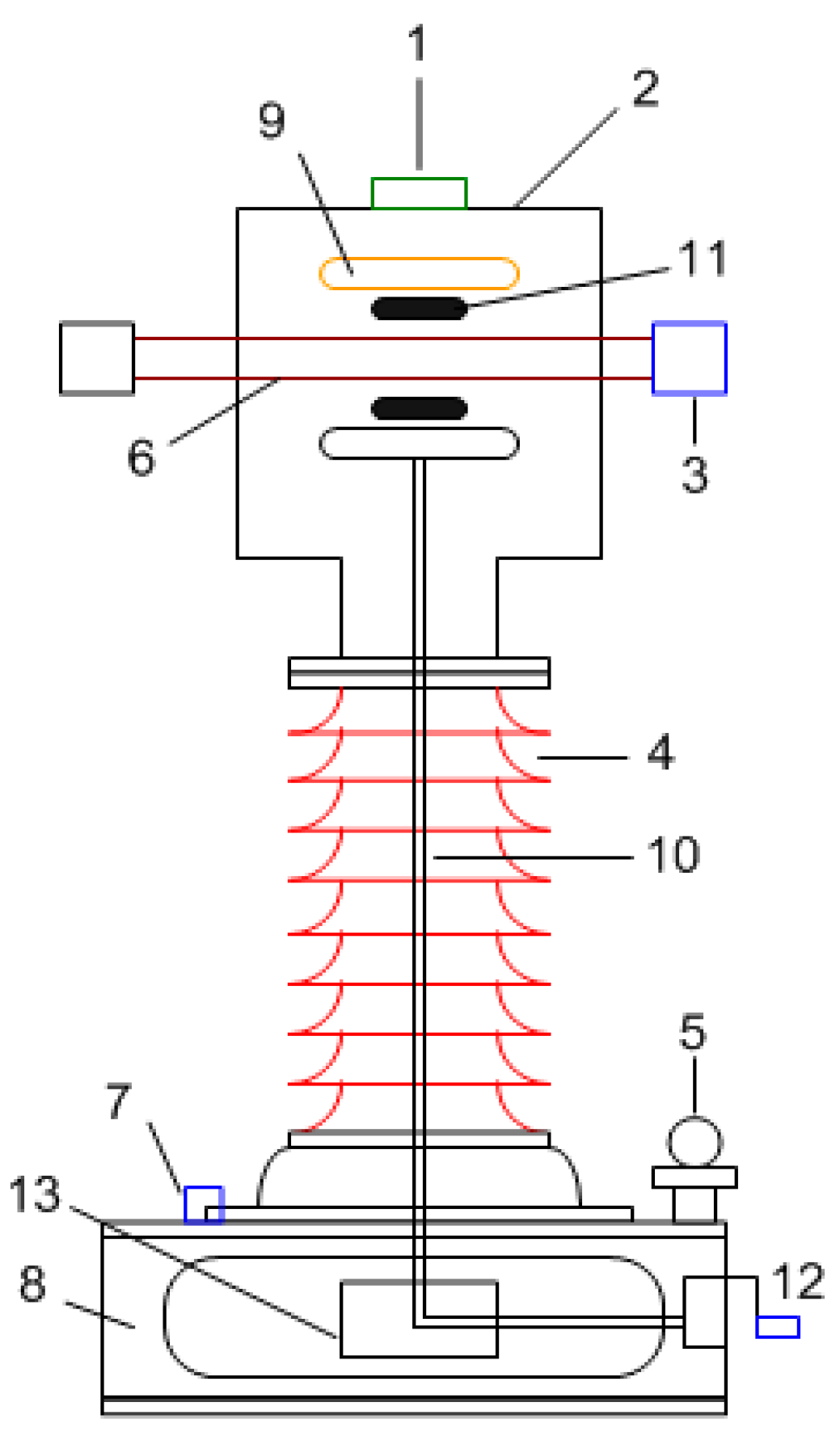
Figure 3.
SF_6 coaxial capacitor structure. 1, metal shield; 2, capacitor ring; 3, primary conductor; 4, high-voltage shell; 5, ground electrode; 6, insulating layer.
Figure 3.
SF_6 coaxial capacitor structure. 1, metal shield; 2, capacitor ring; 3, primary conductor; 4, high-voltage shell; 5, ground electrode; 6, insulating layer.

Figure 4.
Schematic diagram of voltage measurement.

Figure 5.
Romberg algorithm principle.

Figure 6.
Error of the complex rectangle, trapezoid, and Simpson formula.

Figure 7.
Dual-channel digital integrator.

Figure 8.
Schematic diagram of off-axis capacitance.

Figure 9.
Relative change of the capacitance C when the off-axis distance R changes.
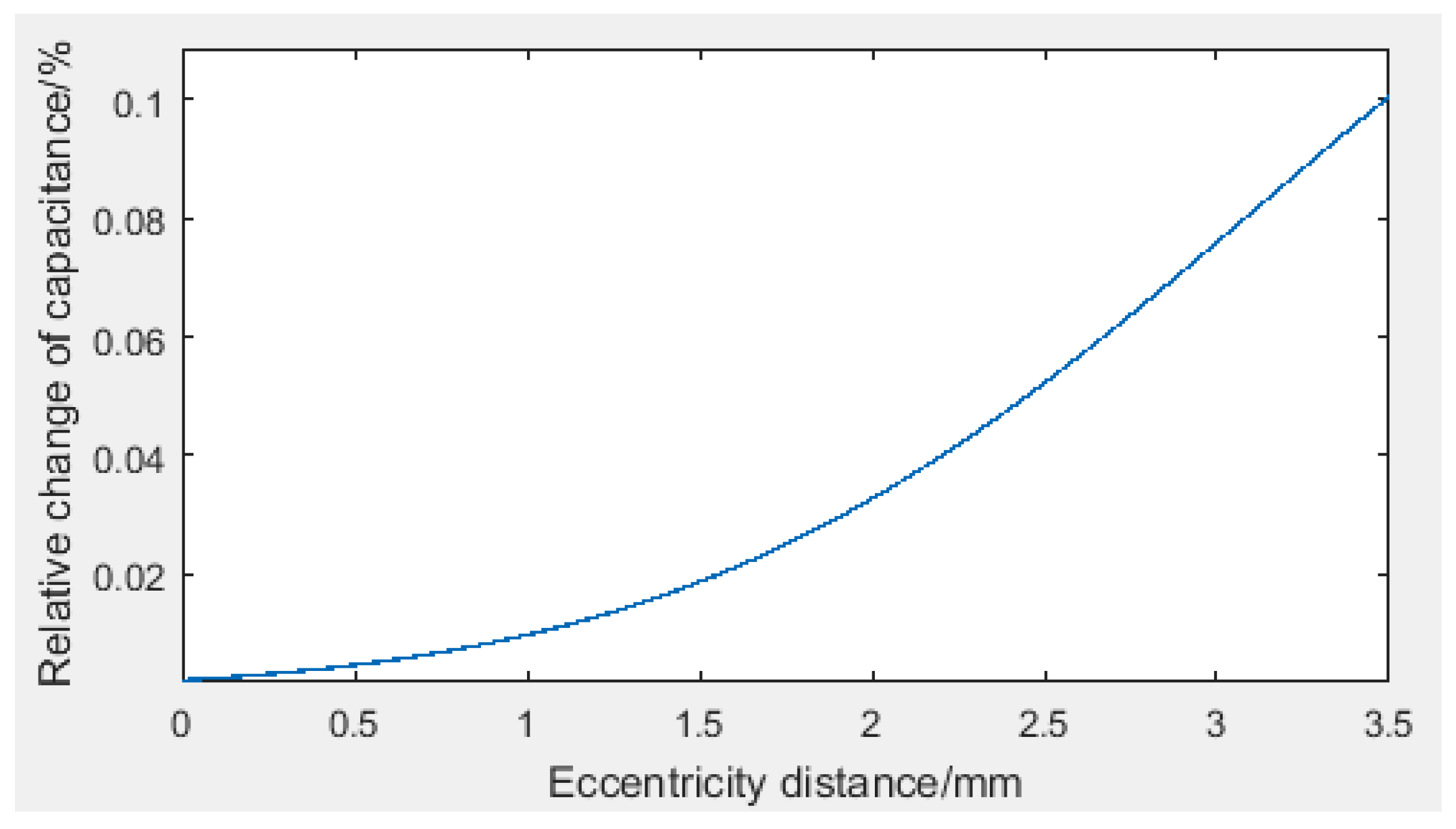
Figure 10.
The change of the capacitance with the temperature when the density is constant.

Figure 11.
The change of the capacitance with the temperature at 1% density change.

Figure 12.
Voltage channel preliminary test and retest data.

Figure 13.
Results of the temperature cycle test.


Table 1.
Error data table.
| n | Complex Rectangular Formula R(n)(0) | Complex Trapezoid Formula R(n)(1) | Complex Simpson Formula R(n)(2) | |||
|---|---|---|---|---|---|---|
| = 0.7 | = 0.95 | = 0.7 | = 0.95 | = 0.7 | = 0.95 | |
| 0 | 0.5771 | 0.8215 | 0.0273 | 0.0754 | 0.0035 | 0.32223 |
| 1 | 0.13902 | 0.19056 | 1.5769 × 10⁻³ | 4.0266 × 10⁻³ | 5.4254 × 10⁻⁶ | 5.7389 × 10⁻⁵ |
Table 2.
Test of partial discharge.
| Standard Requirements | Test Results of the Tested Electronic Voltage Transformer |
|---|---|
| Preload voltage: 230 kV | Preload voltage: 230 kV |
| Test frequency: 50 Hz | Test frequency: 50 Hz |
| Measurement voltage: 126 kV | Measurement voltage: 126 kV |
| Allowable partial discharge: ≤10 pC | apparent charge: 3 pC |
| Measurement voltage: 87 kV | Measurement voltage: 87 kV |
| Allowable partial discharge: ≤5 pC | apparent charge: 2 pC |
Table 3.
Electromagnetic compatibility immunity test.
| Detection Project | Performance Evaluation |
|---|---|
| Voltage variations immunity tests | A |
| Voltage dips and short interruptions immunity tests | A |
| Surge immunity test | A |
| Electrical fast transient/burst immunity test | A |
| Damped oscillatory wave immunity test | A |
| Electrostatic discharge immunity test | A |
| Power frequency magnetic field immunity test | A |
| Pulse magnetic field immunity test | A |
| Damped oscillatory magnetic field immunity test | A |
| Radiated, radio-frequency, electromagnetic field immunity test | A |
© 2018 by the authors. Licensee MDPI, Basel, Switzerland. This article is an open access article distributed under the terms and conditions of the Creative Commons Attribution (CC BY) license (http://creativecommons.org/licenses/by/4.0/).
Share and Cite
MDPI and ACS Style
Li, Z.-H.; Wang, Y.; Wu, Z.-T.; Li, Z.-X. Research on Electronic Voltage Transformer for Big Data Background. Symmetry 2018, 10, 234. https://doi.org/10.3390/sym10070234
AMA Style
Li Z-H, Wang Y, Wu Z-T, Li Z-X. Research on Electronic Voltage Transformer for Big Data Background. Symmetry. 2018; 10(7):234. https://doi.org/10.3390/sym10070234
Chicago/Turabian StyleLi, Zhen-Hua, Yao Wang, Zheng-Tian Wu, and Zhen-Xing Li. 2018. "Research on Electronic Voltage Transformer for Big Data Background" Symmetry 10, no. 7: 234. https://doi.org/10.3390/sym10070234
Note that from the first issue of 2016, this journal uses article numbers instead of page numbers. See further details here.