Joint Adaptive Coding and Reversible Data Hiding for AMBTC Compressed Images

Abstract

This paper proposes a joint coding and reversible data hiding method for absolute moment block truncation coding (AMBTC) compressed images. Existing methods use a predictor to predict the quantization levels of AMBTC codes. Equal-length indicators, secret bits and prediction errors are concatenated to construct the output code stream. However, the quantization levels might not highly correlate with their neighbors for predictive coding, and the use of equal-length indicators might impede the coding efficiency. The proposed method uses reversible integer transform to represent the quantization levels by their means and differences, which is advantageous for predictive coding. Moreover, the prediction errors are better classified into symmetrical encoding cases using the adaptive classification technique. The length of indicators and the bits representing the prediction errors are properly assigned according to the classified results. Experiments show that the proposed method offers the lowest bitrate for a variety of images when compared with the existing state-of-the-art works.

1. Introduction

The rapid development of internet technology has made data security a key consideration for data transmission or content protection. While most digital data can be transmitted over the internet, transmitted data is also exposed to the risks of illegal access or interception. A solution to these problems is to employ a data hiding method, in which secret data are embedded into a digital media to cover the presence of embedment, or to protect the transmitted contents. Data hiding methods for images can be classified into irreversible [1,2,3] and reversible [4,5,6,7] methods. The cover images of both methods are distorted to obtain stego images. However, the distortions of irreversible methods are permanent, and thus, they are not suitable for applications where no distortions are allowed. In contrast, reversible methods recover the original images from the distorted versions after extracting the secret data. Since the original image can be completely recovered, reversible data hiding (RDH) methods have special applications, and much research has been devoted to investigating data hiding methods of this type.

Reversible data hiding method can be applied to images in spatial or compressed domains. The spatial domain methods embed data into a cover image by altering its pixel values. The difference expansion scheme proposed by Tian [8] and the histogram shifting scheme proposed by Ni et al. [9] are two well-known methods of this type. Many recent works [4,5,6,7] have exploited the merits of [8,9] to propose improved methods with better embedding efficiency. In contrast, compressed domain methods modify the coefficients of compressed codes [10], or use the joint neighborhood coding (JNC) [11] scheme to embed data bits into the compressed code stream. Up to now, RDH methods have been applied to vector quantization (VQ) [12,13], joint photographic experts group (JPEG) [14], and absolute moment block truncation coding (AMBTC) [15,16,17,18,19] compressed images. AMBTC [20] is a lossy compression method which re-represents an image block by a bitmap and two quantization levels. As AMBTC requires insignificant compaction costs while achieving satisfactory image quality, some researchers have investigated RDH methods and their applications [21,22,23] in this format.

Zhang et al. [16] in 2013 proposed an RDH for AMBTC compressed images. In their method, the different quantization levels are classified into eight cases, which in turn are recorded by three-bit indicators. By re-representing the AMBTC codes, secret data are embedded into the compressed code stream. Sun et al. [17] also proposed an efficient method using JNC. This method predicts pixel values and obtains prediction errors, which are then classified into four cases. Secret bits, two-bit indicators, and prediction errors are concatenated to construct the output code stream. Hong et al. [18] in 2017 modified the prediction and classification rules from Sun et al.’s work and proposed an improved method with a lower bitrate. However, their method also uses two-bit indicators to represent four categories of prediction errors. The use of equal-length indicators might not efficiently represent the encoding cases, leading to an increase in bitrate. In 2018, Chang et al. [19] also proposed an interesting method to improve Sun et al.’s work. In their method, a neighboring quantization level of the current quantization level, x, is selected as the prediction value, p, to predict x. The prediction error is obtained by performing the exclusive OR operation between the binary representations of p and x, and then the result is converted to its decimal representation. Since the calculated prediction errors are all positive, the sign bits are not required to record them.

In this paper, we propose a new RDH method for AMBTC compressed codes. With the proposed method, the AMBTC compressed image can be recovered, and the embedded data can be completely extracted. Unlike the aforementioned methods that embed data into quantization levels, the proposed method transforms the quantization levels into means and differences, which are used for carrying data bits. Moreover, the classifications of prediction errors are adaptively assigned, and varied length indicators are utilized to effectively reduce the bitrate. The experimental results show that the proposed method achieves the lowest bitrate when compared to recently published works. The rest of this paper is organized as follows. Section 2 briefly introduces the AMBTC compression method as well as Hong et al.’s work. Section 3 presents the proposed method. The experimental results and discussions are given in Section 4, while concluding remarks are addressed in the last section.

2. Related Works

This section briefly introduces the AMBTC compression method. Hong et al.’s work that was published recently is also introduced in this section.

2.1. AMBTC Compression Technique

The AMBTC compression technique partitions an image, I, into blocks of size $r\times r$. The averaged value, ${\left\{v_i\right\}}_{i=1}^N$, of each block, ${\left\{I_i\right\}}_{i=1}^N$, where N is the total number of blocks, is calculated. AMBTC uses the lower and upper quantization levels, denoted by $a_i$ and $b_i$, respectively, and a bitmap, $B_i$, to represent the compressed code of block $I_i$. $a_i$ and $b_i$ are calculated by rounding the averaged result of pixels in $I_i$ with values smaller than, and larger than, or equal to, $v_i$, respectively. The j-th bit in $B_i$, denoted by $B_{i,j}$, is set to ‘1’ if $I_{i,j}\ge v_i$. Otherwise, $B_{i,j}$ is set to ‘0’. Every block is processed in the same manner, and the final AMBTC code, ${\{a_i,b_i,B_i\}}_{i=1}^N$, is obtained. The decoding of AMBTC codes can be done by simply replacing the bits valued ‘0’ by $a_i$ and the bits valued ‘1’ by $b_i$. A simple example is given below. Let $I_i$ = [23,45,46,47; 43,47,77,80; 88,86,78,90; 78,80,68,70] be an image block to be compressed, where the semicolon denotes the end-of-row operator. The averaged value of $I_i$ is 65.38. The averaged value of pixels with values larger than or equal to 65.38 is 79.50. Therefore, we obtain $b_i=80$. Likewise, the averaged value of pixels with values less than 65.38 is 41.83 and thus, $a_i=42$. Finally, the bitmap obtained is $B_i$ = [0000; 0011; 1111; 1111]. The decoded AMBTC block of the compressed code {42,80, [0000; 0011; 1111; 1111]} is [42,42,42,42; 42,42,80,80; 80,80,80,80; 80,80,80,80].

2.2. Hong et al.’s Method

In 2017, Hong et al. [18] proposed an efficient data hiding method for AMBTC compressed images. Their method uses the median edge detection (MED) predictor to obtain the prediction values as follows. Let x be the to-be-predicted upper or lower quantization level, and $x_u$, $x_{\ell }$, and $x_{u\ell }$ be the quantization levels to the upper, left, and upper left of x, respectively. The MED predictor predicts x using the following rule to obtain the prediction value. p:

$$p=\{\begin{array}{ll}\min (x_u,x_{\ell }),\hfill & x_{u\ell }\ge \max (x_u,x_{\ell });\hfill \\ \max (x_u,x_{\ell }),\hfill & x_{u\ell }\le \min (x_u,x_{\ell });\hfill \\ x_u+x_{\ell }-x_{u\ell },\hfill & \mathrm{otherwise}.\end{array}$$

(1)

The prediction error, e, calculated by $e=x-p$, is classified into four categories using the centralized error division (CED) technique. Two-bit indicators, ‘00’, ’01’, ‘10’, and ‘11’, are used to specify four corresponding encoding cases. The first case occurs when $e=0$. In this case, the prediction error does not need bits to be recorded. The n-bit secret data, ${\left\{s_j\right\}}_{j=1}^n$, and the indicator ‘00’ are concatenated together and output the result, ${\left\{s_j\right\}}_{j=1}^n$||00 to the code stream, CS. The second case occurs if $1\le e\le 2^{\beta }$. In this case, the bitstream, ${\left\{s_j\right\}}_{j=1}^n$||01||${(e-1)}_2^{\beta }$, is outputted to the CS, where ${(y)}_2^k$ represents the k-bit binary representation of $y$, and the symbol || is the concatenation operator. Similarly, if $-(2^{\beta })\le e\le -1$ (the third case), ${\left\{s_j\right\}}_{j=1}^n$||10||${(-e-1)}_2^{\beta }$ is outputted to the CS. The last case occurs when $e>2^{\beta }$ or $e<-2^{\beta }$. In this case, ${\left\{s_j\right\}}_{j=1}^n$||11||${(x)}_2^8$ is output. The detailed encoding and decoding procedures can be found in [18].

3. Proposed Method

The existing RDH methods for AMBTC compressed images [16,17,18,19] all perform predictions on the quantization levels of AMBTC codes. The prediction errors are classified into categories. The secret data bits, indicators, and prediction errors are then concatenated and output to the code stream. For the JNC technique, better prediction often results in a smaller bitrate since fewer bits are required to record the prediction errors. However, the existing methods all perform the prediction on two quantization levels, which might not correlate enough to obtain a good prediction result. Moreover, this classification of prediction errors does not consider their distributions and assigns the same classification rules to different images. Improper classification might lead to a significant increase in bitrate. The proposed method transforms pairs of quantization levels into their means and differences using the reversible integer transform (RIT). The transformed means and differences are generally more correlated than the quantization levels, and thus, they are more suitable for predictive coding. The prediction errors are adaptively classified according to their distribution, ensuring that fewer bits are required to record them. Techniques used this paper will be separately introduced in the following two subsections.

3.1. Reversible Integer Transform of Quantization Levels

A pair of quantization levels $(a_i,b_i)$ can be transformed into their mean, $m_i$, and difference, $d_i$, using transform:

$$m_i=\lfloor \frac{a_i+b_i}{2}\rfloor ,d_i=b_i-a_i,$$

(2)

where $\lfloor ·\rfloor$ is the floor operator. The transformation in Equation (2) is reversible since the pair of quantization levels, $(a_i,b_i)$, can be recovered by the inverse transform:

$$a_i=m_i-\lfloor \frac{d_i}{2}\rfloor ,b_i=m_i+\lfloor \frac{d_i+1}{2}\rfloor .$$

(3)

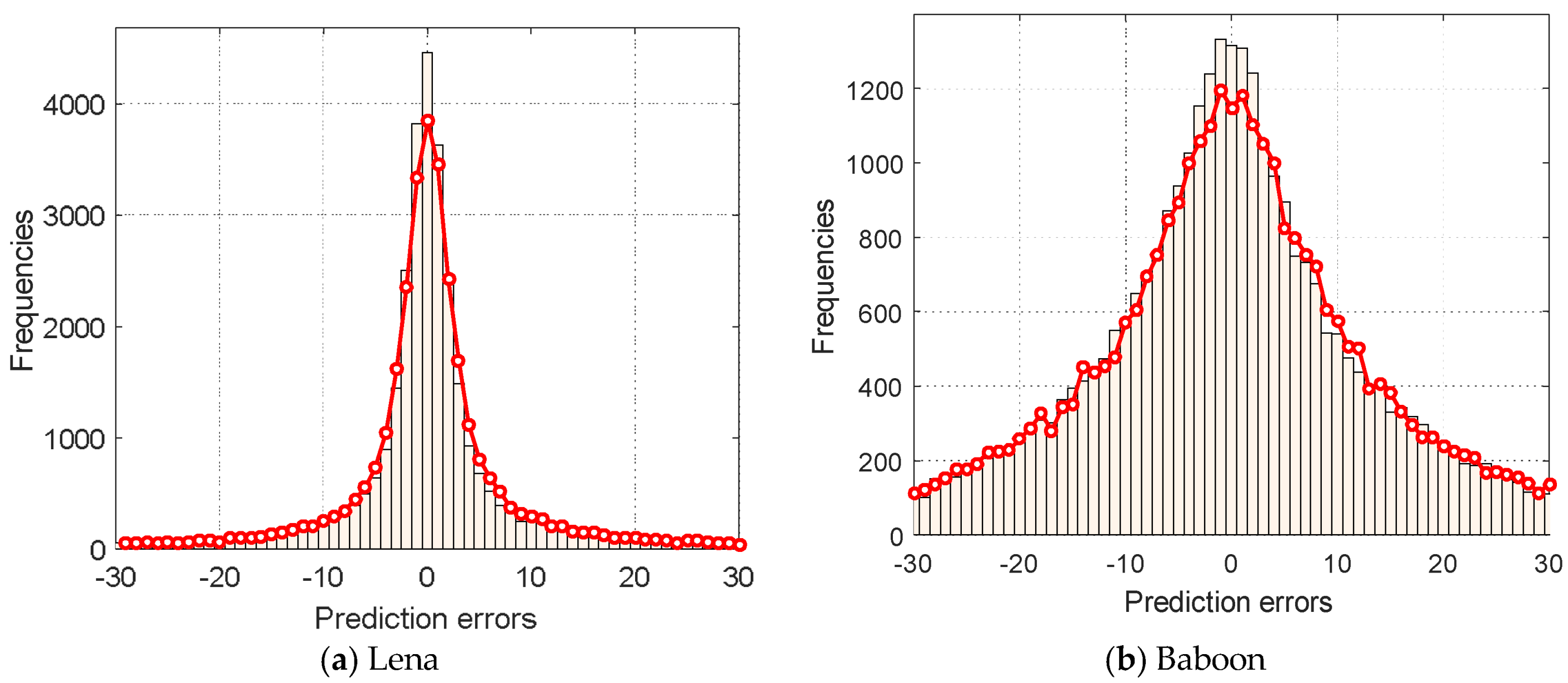
Since the mean operation has a tendency to reduce the noise, and the difference operation tends to reduce the variation in neighboring quantization levels, the transformed means and differences are often more correlated than the quantization levels. Therefore, the prediction performed on the means and differences will improve the prediction accuracy. Figure 1 shows the distribution of prediction errors for the Lena and Baboon images using the MED predictor. In this figure, the red line with circle marks is the predictor that is applied on the upper and lower quantization levels, whereas the histogram is the prediction result when the predictor is applied on the transformed means and differences. As seen from Figure 1, the peak of the histogram is higher than that of the red circle line for both Lena and Baboon images. In fact, the experiments on other test images also obtain similar trends, indicating that the transformed means and differences are more amenable for predictive coding.

3.2. Adaptive Case Classification Technique

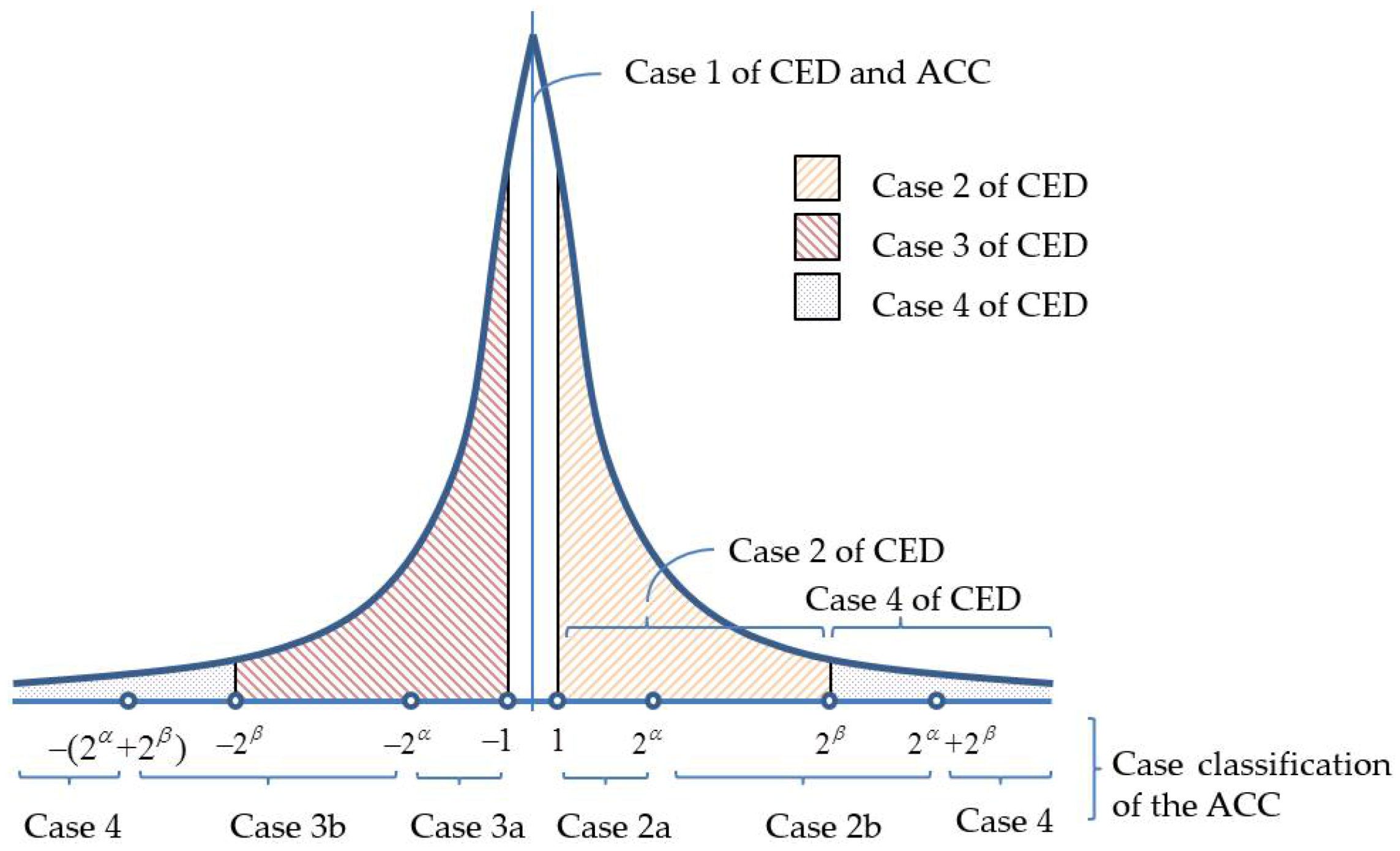
In Hong et al.’s CED technique [18], the encoding of a prediction error, $e$, is classified into four cases. If $1\le e\le 2^{\beta }$ (case 2), $e$ is encoded by a $\beta -\mathrm{bit}$ plus a two-bit indicator. Therefore, a total of $2+\beta$ bits are required to encode a case-2 prediction error. Figure 2 shows a typical prediction error histogram, and the distribution has a sharp peak at zero and decays exponentially towards two sides. The prediction errors fall in case 2 of [18] is shaded by and each requires $\beta$ bits to record its value. However, the occurring frequencies of prediction errors in the range of $1\le e\le 2^{\beta }$ vary significantly. Within this range, the occurring frequency is the highest at $e=1$, in general, and decreases exponentially towards $e=2^{\beta }$. Therefore, the recording of prediction errors using $\beta$ bits in this range with unbalanced frequencies is likely to increase the bitrate. The encoding of case 3 prediction errors, used in [18], also had similar problems.

We propose an adaptive case classification (ACC) technique to better classify the encoding cases. By dividing cases 2 and 3 used in the CED technique into sub-cases, the overall encoding efficiency can be significantly increased. Let x be the to-be-encoded elements and p be the prediction value of x using the MED predictor. The prediction error, e, can be calculated by $e=x-p$. Similar to the CED, the ACC classifies $e=0$ into case 1, and no bits are required to record the prediction errors. Case 2 in the proposed ACC technique is sub-divided into case 2a ($1\le e\le 2^{\alpha }$) and case 2b ($2^{\alpha }+1\le e\le 2^{\alpha }+2^{\beta }$), where $\alpha$ and $\beta$ ($\alpha <\beta$) are the number of bits used to record the prediction errors of cases 2a and 2b, respectively. Similarly, case 3a ($-2^{\alpha }\le e\le -1$) and case 3b ($-(2^{\alpha }+2^{\beta })\le e\le (2^{\alpha }+1$) are the subcases of case 3, and the ACC respectively uses $\alpha$ and $\beta$ bits to record the prediction errors of these two cases. Finally, case 4 occurs when or $e\le -(2^{\alpha }+2^{\beta }+1)$. In this case, we directly record the eight-bit binary representation of x. We use two- or three-bit indicators to indicate the encoding cases. The indicator used for each case, the associated ranges of prediction errors, and the corresponding code length (exclude the secret data) are shown in

Table 1. Indicators and the range of cases.

Case		Indicator	Range of Prediction Errors	Code Length
case 1		‘00’	$e=0$	2
case 2	case 2a	‘010’	$1\le e\le 2^{\alpha }$	$3+\alpha$
	case 2b	‘011’	$2^{\alpha }+1\le e\le 2^{\alpha }+2^{\beta }$	$3+\beta$
case 3	case 3a	‘100’	$-2^{\alpha }\le e\le -1$	$3+\alpha$
	case 3b	‘101’	$-(2^{\alpha }+2^{\beta })\le e\le -(2^{\alpha }+1)$	$3+\beta$
case 4		‘11’	$e\ge 2^{\alpha }+2^{\beta }+1$ or $e\le -(2^{\alpha }+2^{\beta }+1)$	$2+8=10$

.

The advantages of using the ACC over the CED technique are as follows. When $1\le e\le 2^{\alpha }$, $\beta$ bits are required to record the prediction errors in the CED technique. However, the ACC technique only requires $\alpha$ bits plus one extra bit to distinguish the sub-case. As a result, the ACC technique saves $\beta -\alpha -1$ bits if $1\le e\le 2^{\alpha }$. When $2^{\alpha }+1\le e\le 2^{\beta }$, both techniques require $\beta$ bits to record the prediction errors. However, the ACC technique requires one more bit to distinguish the sub-case. When $2^{\beta }+1\le e\le 2^{\alpha }+2^{\beta }$, the CED technique requires eight bits to record the prediction errors whereas the ACC technique requires only $\beta$ bits. Therefore, in this range, the ACC technique saves $8-\beta -1$ bits. Although the analyses above are focused on case 2 of Hong et al.’s CED technique, the results also hold for case 3 in their method since the prediction error histograms are often symmetrically distributed.

Since all of the prediction errors can be obtained by pre-scanning the transformed means and differences, the bitrate can be pre-estimated prior to the encoding and embedding processes. Therefore, the best parameters, denoted by $\alpha$ and $\beta$, that minimize the bitrate can be simply obtained by varying their values within a small range while pre-estimating the bitrate. According to our experiments, setting $1\le \alpha \le 3$ and $3\le \beta \le 5$ is sufficient to obtain the best values. Figure 3 shows the effect of the proposed ACC technique applied on the Lena image with $\alpha =2$ and $\beta =4$. In this figure, the red dots and red circles represent that the proposed method saves $\beta -\alpha -1=1$ and $8-\beta -1=3$ bits when recording the prediction errors, respectively. In contrast, the blue cross marks represents that one more bit is required in the proposed ACC technique to record the prediction errors. As shown in this figure, the number of red dots and circles is significantly more than that of blue cross marks, indicating that the ACC technique indeed effectively reduces the bitrate.

3.3. The Embedding Procedures

In this section, we describe the embedment of secret data, S, in detail. Let ${\{a_i,b_i,B_i\}}_{i=1}^N$ be the AMBTC codes to be embedded. An empty array, CS, is initialized to store the code stream. The MED predictor described in Section 2.2 is employed to predict the visited elements. The step-by-step embedding procedures are listed as follows.

Step 1:

Transform the quantization levels, ${\left\{a_i\right\}}_{i=1}^N$ and ${\left\{b_i\right\}}_{i=1}^N$, into means, ${\left\{m_i\right\}}_{i=1}^N$, and differences, ${\left\{d_i\right\}}_{i=1}^N$, using the RIT technique, as described in Section 3.1.

Step 2:

Visit ${\left\{m_i\right\}}_{i=1}^N$ and ${\left\{d_i\right\}}_{i=1}^N$ sequentially, and use the ACC technique described in Section 3.2 to find the best $\alpha$ and $\beta$ values, such that the estimated code length is minimal.

Step 3:

Convert the elements in the first row and the first columns of ${\left\{m_i\right\}}_{i=1}^N$ and ${\left\{d_i\right\}}_{i=1}^N$ to their eight-bit binary representations. The converted results are appended to the CS.

Step 4:

Scan the rest elements in ${\left\{m_i\right\}}_{i=1}^N$ using the raster scanning order and use the MED predictor (Equation (1)) to predict scanned $m_i$. Let $p_i$ be the prediction value and calculate the prediction error $e_i=m_i-p_i$.

Step 5:

Extract n-bit secret data, ${\left\{s_j\right\}}_{j=1}^n$, from S. In accordance with $e_i$, one of the four encoding cases is applied:

Case 1:

If $e_i=0$, the bits ${\left\{s_j\right\}}_{j=1}^n$||00 are append to the code stream, CS.

Case 2:

If $1\le e_i\le 2^{\alpha }$, append the bits, ${\left\{s_j\right\}}_{j=1}^n$||010||${(e_i-1)}_2^{\alpha }$, to the CS, where ${(y)}_2^k$ is the $k-\mathrm{bit}$ binary representation of y. If $2^{\alpha }+1\le e_i\le 2^{\alpha }+2^{\beta }$, append ${\left\{s_j\right\}}_{j=1}^n$||011||${(e_i-2^{\alpha }-1)}_2^{\beta }$ to the CS.

Case 3:

If $-2^{\alpha }\le e_i\le -1$, append the bits, ${\left\{s_j\right\}}_{j=1}^n$||100||${(-e_i-1)}_2^{\alpha }$, to the CS. If $-(2^{\alpha }+2^{\beta })\le e_i\le -(2^{\alpha }+1)$, append ${\left\{s_j\right\}}_{j=1}^n$||101||${(-e_i-2^{\alpha }-1)}_2^{\beta }$ to the CS.

Case 4:

If $e_i\le -(2^{\alpha }+2^{\beta }+1)$ or $e_i\ge 2^{\alpha }+2^{\beta }+1$, append the bits, ${\left\{s_j\right\}}_{j=1}^n$||11||${(m_i)}_2^8$, to the CS.

Step 6:

Repeat Steps 4–5 until all means, ${\left\{m_i\right\}}_{i=1}^N$, are encoded.

Step 7:

Use the same procedures listed in Steps 4–6 to encode the differences, ${\left\{d_i\right\}}_{i=1}^N$, and append the encoded result to the CS.

Step 8:

Append the bitmap, ${\left\{B_i\right\}}_{i=1}^N$, to the CS, to construct the final code stream, $C{S}_f$.

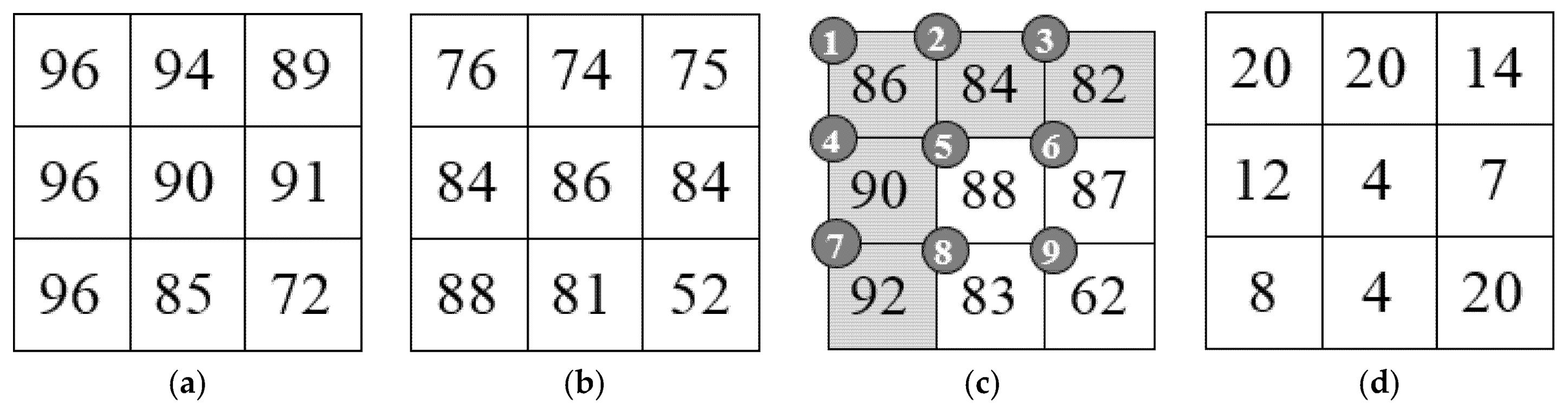
We use a simple example to illustrate the embedding procedures of the proposed method. Suppose the AMBTC codes consist of $3\times 3$ upper and lower quantization levels, as shown in Figure 4a,b, respectively. Let $S={\left\{s_j\right\}}_{j=1}^8$ = ‘10111001’ be the secret data and suppose $\alpha =2$, $\beta =4$. Firstly, we convert the quantization levels into means, ${\left\{m_i\right\}}_{i=1}^9$, and differences, ${\left\{d_i\right\}}_{i=1}^9$, using Equation (2). The converted results are shown in Figure 4c,d.

To encode the means ${\left\{m_i\right\}}_{i=1}^9$ and embed S, convert the elements in the first row and the first column (elements numbered 1, 2, 3, 4, and 7) of ${\left\{m_i\right\}}_{i=1}^9$ are converted to their eight-bit binary representations. In this example, we only focus on the encoding of elements $m_5$, $m_6$, $m_8$, and $m_9$ (the elements numbered 5, 6, 8, and 9). To encode $m_5=88$, we use Equation (1) to predict $m_5$ and obtain the prediction value, $p_5=88$. Therefore, we have the prediction error, $e_5=0$, which is classified into case 1, and the associated indicator is ${00}_2$. Two bits, ${\left\{s_j\right\}}_{j=1}^2={10}_2$, are extracted from S, and ${\left\{s_j\right\}}_{j=1}^2$ and the case 1 indicator are concatenated, to obtain the codes for the fifth element, 10||00. The prediction value, $p_6$, of $m_6=87$ is 86, and thus, $e_6=87-86=1$. Since $1\le e_6\le 2^{\alpha }=4$, case 2a should be applied to encode $m_6$. The third and fourth bits, ${\left\{s_j\right\}}_{j=3}^4={11}_2$, are extracted from S, and ${\left\{s_j\right\}}_{j=3}^4$, the case 2a indicator ‘010’ and the $\alpha =2$ bits binary representation of $e_6-1$ are concatenated, giving 11||010||00. To encode $m_8=83$, since $p_8=90$ and $e_8=-7$, we have to use case 3b to encode $m_8$. ${\left\{s_j\right\}}_{j=5}^6={10}_2$ is extracted from S, and ${\left\{s_j\right\}}_{j=5}^6$, the case 3b indicator ‘101’, and the $\beta -\mathrm{bit}$ binary representation of $-e_8-2^{\alpha }-1=2$ are concatenated, giving 10||101||0010. Finally, since the prediction value of $m_9$ is $p_9=83$, we have $e_9=62-83=-21$, which is categorized as case 4. Therefore, the encoded result of $m_9$ is 01||11||00111110. The coded results of $m_5$, $m_6$, $m_8$, and $m_9$ are concatenated and the code stream 1000||1101000||101010010||011100111110 is obtained. The code stream of ${\left\{d_i\right\}}_{i=1}^9$ can be encoded using the similar manner, but the detailed steps for this are omitted in this example.

3.4. The Extraction and Recovery Procedures

Once the receiver has the final code stream, $C{S}_f$, the embedding parameters, $\alpha$, $\beta$, and n, the embedded secret data, S, can be extracted, and the original AMBTC codes, ${\{a_i,b_i,B_i\}}_{i=1}^N$, can be recovered. The detailed extraction and recovery procedures are listed as follows.

Step 1:

Prepare empty arrays ${\left\{a_i\right\}}_{i=1}^N$, ${\left\{b_i\right\}}_{i=1}^N$, ${\left\{m_i\right\}}_{i=1}^N$, ${\left\{d_i\right\}}_{i=1}^N$, and S for storing the reconstructed lower quantization levels, upper quantization levels, means, differences, and secret data, respectively.

Step 2:

Read eight bits sequentially from $C{S}_f$ and convert them into integers. Place the converted integers in the first row and the first column of ${\left\{m_i\right\}}_{i=1}^N$.

Step 3:

Read the next n bits from $C{S}_f$ and append them to S.

Step 4:

Visit the unrecovered means, $m_i$, in ${\left\{m_i\right\}}_{i=1}^N$ using the raster scanning order. Use Equation (1) to predict $m_i$, and obtain the prediction value, $p_i$.

Step 5:

Read the next two bits, ${\left\{t_j\right\}}_{j=1}^2$, from $C{S}_f$, and use the following rules to recover $m_i$:

Case 1:

If ${\left\{t_j\right\}}_{j=1}^2=$‘00’, $m_i=p_i$.

Case 2:

If ${\left\{t_j\right\}}_{j=1}^2=$‘01’, read the next bit, $t$, from $C{S}_f$. If $t$ = ‘0’, read the next $\alpha$ bits, ${\left\{t_j\right\}}_{j=1}^{\alpha }$, from $C{S}_f$. The mean, $m_i$, is recovered by $m_i=p_i+{({\left\{t_j\right\}}_{j=1}^{\alpha })}_{10}+1$, where ${(y)}_{10}$ represents the decimal value of bitstream y. If $t$ = ‘1’, read the next $\beta$ bits ${\left\{t_j\right\}}_{j=1}^{\beta }$ from $C{S}_f$. The mean, $m_i=p_i+{({\left\{t_j\right\}}_{j=1}^{\beta })}_{10}+2^{\alpha }+1$, is recovered.

Case 3:

If ${\left\{t_j\right\}}_{j=1}^2=$‘10’, read the next bit, $t$, from $C{S}_f$. If $t$ = ‘0’, read the next $\alpha$ bits, ${\left\{t_j\right\}}_{j=1}^{\alpha }$, from $C{S}_f$. The mean, $m_i$, is recovered by $m_i=p_i-{({\left\{t_j\right\}}_{j=1}^{\alpha })}_{10}-1$. If $t$ = ‘1’, read the next $\beta$ bits, ${\left\{t_j\right\}}_{j=1}^{\beta }$, from $C{S}_f$. The mean, $m_i=p_i-{({\left\{b_j\right\}}_{j=1}^{\beta })}_{10}-2^{\alpha }-1$, is recovered.

Case 4:

If ${\left\{t_j\right\}}_{j=1}^2$= ‘11’, read the next eight bits ${\left\{t_j\right\}}_{j=1}^8$ from $C{S}_f$, and the mean,$m_i={({\left\{t_j\right\}}_{j=1}^8)}_{10}$, is recovered.

Step 6:

Perform Steps 3–5 until all the means ${\left\{m_i\right\}}_{i=1}^N$ are recovered.

Step 7:

Recover the differences ${\left\{d_i\right\}}_{i=1}^N$ and extract data bits embedded in ${\left\{d_i\right\}}_{i=1}^N$. The procedures are similar to Steps 2–6.

Step 8:

Extract the remaining bits in $C{S}_f$ and rearrange them to obtain ${\left\{B_i\right\}}_{i=1}^N$. Transform ${\left\{m_i\right\}}_{i=1}^N$ and ${\left\{d_i\right\}}_{i=1}^N$ into ${\left\{a_i\right\}}_{i=1}^N$ and ${\left\{b_i\right\}}_{i=1}^N$ using Equation (3); the original AMBTC codes, ${\{a_i,b_i,B_i\}}_{i=1}^N$, can be reconstructed.

We continue the example given in Section 3.3 to illustrate the procedures of the extraction of S and the recovery of the quantization levels. Suppose the first row and the first column of the means ${\left\{m_i\right\}}_{i=1}^9$ have been recovered (see Figure 4c), and the code stream, CS, to be decoded is 1000||1101000||101010010||011100111110. The first two bits, ${\left\{t_j\right\}}_{j=1}^2$ = ‘10’, are read from CS and placed in an empty array S. The MED predictor is used to predict $m_5$; we have $p_5=88$. The next two bits are ‘00’, and thus, the prediction error is $e_5=0$. Therefore, $m_5=p_5=88$. The next two bits, ‘11’, are read and appended to S. The next two bits, ‘01’, are read from CS, and the next bit read is ‘0’. Therefore, $m_6$ is encoded using case 2a. The next $\alpha =2$ bits, ${\left\{t_j\right\}}_{j=1}^2$ = ‘00’, are read from CS; we have $e_6={({\left\{t_j\right\}}_{j=1}^2)}_{10}+1=1$. Since $p_6=86$, we have $m_6=p_6+e_6=87$. The next two bits are read from CS and appended to S. Because the next three bits from CS are ‘101’, $m_8$ is encoded using case 3b. The next $\beta =4$ bits, ${\left\{t_j\right\}}_{j=1}^4$ = ‘0010’, are read from CS; we have $e_8={({\left\{t_j\right\}}_{j=1}^4)}_{10}+2^2+1=7$. Therefore, $m_8=p_8-e_8=90-7=83$, where $p_8$ is obtained using the MED predictor. Finally, two bits, ‘01’, are read from CS and appended to S. The next two bits are ‘11’, and thus, $m_9$ can be obtained by converting the next eight bit to its decimal representation; we have $m_9=62.$ Therefore, the means, ${\left\{m_i\right\}}_{i=1}^9$, can be recovered (Figure 4c). Similarly, the differences, ${\left\{d_i\right\}}_{i=1}^9$, can also be recovered (Figure 4d). Finally, according to Equation (3), the original upper and lower quantization levels can be recovered from ${\left\{m_i\right\}}_{i=1}^9$ and ${\left\{d_i\right\}}_{i=1}^9$. The recovered quantization levels are shown in Figure 4a,b.

4. Experimental Results

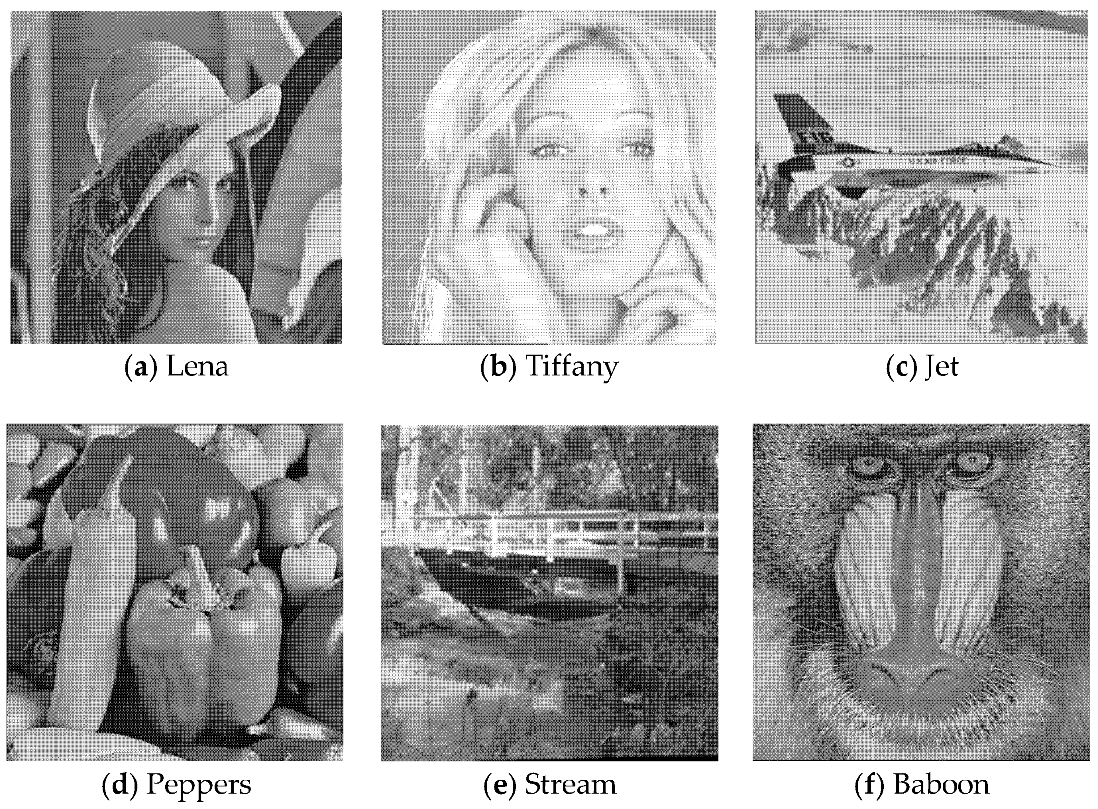
In this section, we conduct several experiments and compare the results with some other state-of-the-art works to evaluate the performance of the proposed method. Six $512\times 512$ grayscale images shown in Figure 5, including Lena, Tiffany, Jet, Peppers, Stream, and Baboon, were used as the test images to generate the AMBTC codes. These images can be obtained from [24].

The peak signal-to-noise ratio (PSNR) metric was used to measure the quality of AMBTC compressed image. To make a fair comparison, the pure bitrate, $B{R}_p$, metric, which is defined by

$$B{R}_p=\frac{\left|C{S}_f\right|-\left|S\right|}{\mathrm{Total}\mathrm{number}\mathrm{of}\mathrm{pixels}\mathrm{of}\mathrm{the}\mathrm{original}\mathrm{image}},$$

(4)

was used to measure the embedding performance, where $\left|C{S}_f\right|$ and $\left|S\right|$ are the length of final code stream, $C{S}_f$, and secret data, S, respectively. In fact, the pure bitrate measures the number of bits required to record a pixel in the original image. Therefore, this metric should be as low as possible.

4.1. Performance Evaluation of the Proposed Method

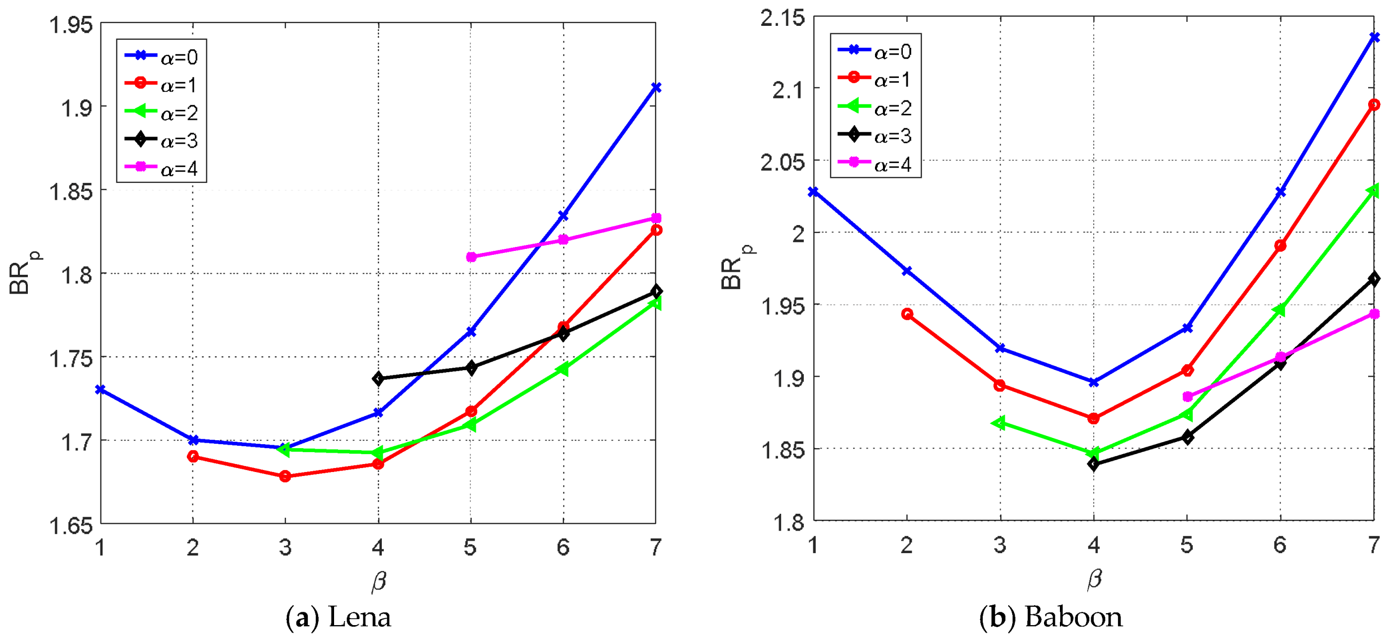
Figure 6a,b shows the pure bitrate, $B{R}_p$, versus parameter $\beta$ under various $\alpha$ for the Lena and Baboon images. As seen from the figures, setting $\alpha =1$ and $\beta =3$ for the Lena image achieved the lowest bitrate. However, $\alpha =3$ and $\beta =4$ had to be set for the Baboon image to achieve the best result. This is because the prediction error histogram of the Lena image is sharper than that of the Baboon image, forcing the ACC technique to select smaller $\alpha$ and $\beta$ values. In contrast, the prediction error histogram of the Baboon image is flatter than that of the Lena image, and thus larger $\alpha$ and $\beta$ are selected.

Table 2. The combination of $\alpha$ and $\beta$ to achieve the lowest bitrates.

Images	Lena	Tiffany	Jet	Peppers	Stream	Baboon
$(\alpha ,\beta )$	(1,3)	(1,3)	(1,3)	(1,3)	(3,4)	(3,4)
$B{R}_p$	1.68	1.64	1.67	1.68	1.83	1.84

gives the best $\alpha$ and $\beta$ values for the six test images. Notice that the values of $\alpha$ and $\beta$ tended to be smaller for smooth images than those of complex images.

The proposed method classifies prediction errors into four encoding cases, and each case requires a different number of bits to record the prediction error. Figure 7 shows the distributions of these cases when the ACC technique is applied on the transformed means with $\alpha =1$ and $\beta =3$. In this figure, the red circles, blue crosses, green dots, and black squares representing the corresponding means are encoded using case 1, 2a or 3a, 2b or 3b, and 4, respectively.

Figure 7 shows that the smooth parts of the Lena images are filled with red circles and blue crosses, indicating that they are encoding using case 1, 2a, or 3a. The texture areas or edges of the Lena image are filled with black squares, meaning that the complex parts of the Lena image are encoded by case 4. It is interesting to note that most of the green dots are in the vicinity of the black squares. This indicates that the areas occupied by the green dots are less complex than those of black squares and thus, the corresponding means are encoded by case 2b or 3b.

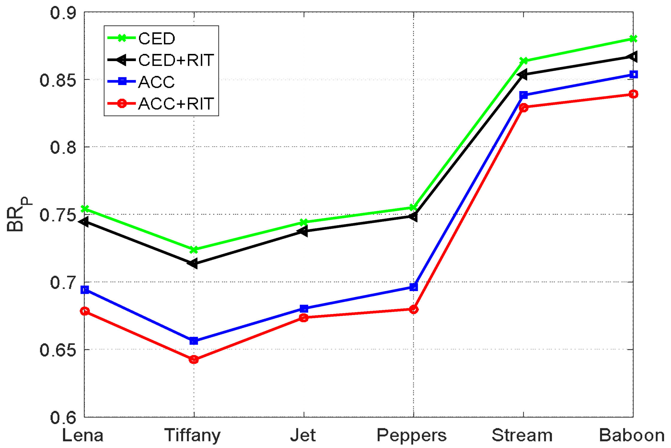
The proposed method uses the RIT technique to convert quantization levels into means and differences, and the ACC technique is then applied to encode the transformed values. To see how these two techniques affect the encoding performance, the pure bitrate is plotted in Figure 8 for all test images under various combinations of techniques. In this figure, the lines labeled ‘CED’ indicate that the CED technique with $\beta =4$ was applied on the prediction errors obtained from predicting the quantization levels. In contrast, ‘CED + RIT’ represents that the CED was applied on the prediction errors obtained from the proposed RIT technique. The line labeled ‘ACC’ indicates that the ACC technique was applied on the two quantization levels, and ‘ACC + RIT’ is the result when both ACC and RIT techniques have been applied. For the ACC technique, the best $\alpha$ and $\beta$ listed in Table 2 were used.

As seen from Figure 8, the bitrate obtained by the ‘CED’ method was the largest. When the CED together with the RIT technique was applied, all the bitrates of the six test images were reduced, meaning that the transformed means and differences are more suitable for predictive coding than the original quantization levels. However, when the ACC technique was applied on the quantization levels, the reduction in bitrate was more significant, indicating that the ACC technique reduces the bitrate considerably. The best result was achieved when both ACC and RIT techniques were applied. It is interesting to note that the improvement of smooth images is more significant than that of complex images when using the proposed ‘ACC + RIT’ technique. The reason for this is that the proposed method saves $\beta -\alpha -1$ bits when the predication errors are categorized as case 2a or 3a but requires one additional bit when they are categorized as case 2b or 3b. Since the prediction errors categorized as case 2a or 3a are more frequent in smooth images than complex images, we can infer that the proposed method works better for smooth images.

4.2. Comparison with Other Works

In this section, we compare some related works that have been published recently, including Zhang et al.’s [16], Sun et al.’s [17], Hong et al.’s [18], and Chang et al.’s [19] methods. In Zhang et al.’s method, eight cases for coding the differences are implemented to achieve the best result. In Sun et al.’s and Hong et al.’s methods, the best embedding parameters are set to obtain the lowest bitrate, as suggested in their original paper. In Chang et al.’s method, the exclusive OR operation is employed to generate the prediction errors. In the proposed method, the best $\alpha$ and $\beta$ that minimize the bitrate are selected for embedment. All the settings used ensured that the best performance could be achieved for each compared method. The results are shown in

Table 3. Comparisons with other works.

Metric	Methods	Lena	Tiffany	Jet	Peppers	Stream	Baboon
PSNR		33.24	35.77	31.97	33.42	28.59	26.98
Payload	[16]	32,768	32,768	32,768	32,768	32,768	32,768
	[17]	64,008	64,008	64,008	64,008	64,008	64,008
	[18]	64,516	64,516	64,516	64,516	64,516	64,516
	[19]	64,008	64,008	64,008	64,008	64,008	64,008
	Proposed	64,516	64,516	64,516	64,516	64,516	64,516
Embedding Efficiency	[16]	0.066	0.067	0.066	0.065	0.062	0.063
	[17]	0.116	0.118	0.116	0.116	0.111	0.112
	[18]	0.123	0.125	0.124	0.123	0.117	0.116
	[19]	0.118	0.121	0.119	0.118	0.112	0.113
	Proposed	0.128	0.130	0.128	0.128	0.119	0.118
Pure Bitrate	[16]	1.77	1.75	1.76	1.79	1.88	1.87
	[17]	1.86	1.82	1.86	1.86	1.95	1.94
	[18]	1.75	1.72	1.74	1.76	1.86	1.88
	[19]	1.82	1.78	1.80	1.83	1.94	1.92
	Proposed	1.68	1.64	1.67	1.68	1.83	1.84

.

In Table 3, the PSNR metric measured the image quality of AMBTC compressed images. The payload was designed such that each quantization level carried two data bits, apart from methods that can only carry one bit per quantization level (e.g., Zhang et al.’s method). The embedding efficiency is defined by $\left|S\right|/\left|C{S}_f\right|$, which indicates how many secret data bits can be carried per bit of code stream. Therefore, the larger the embedding efficiency, the better the performance is. We also compared the pure bitrate for all the methods. The results show that the proposed method achieves the highest embedding efficiency with the lowest pure bitrate. This is due to the subtly transformation of the quantization levels into means and differences, and the performance of predictive coding together with the ACC technique on the transformed domain. In contrast, the other compared methods all perform the prediction on the original quantization level, and the encoding cases are not adaptively designed. Therefore, their achieved pure bitrates are higher than that of the proposed method.

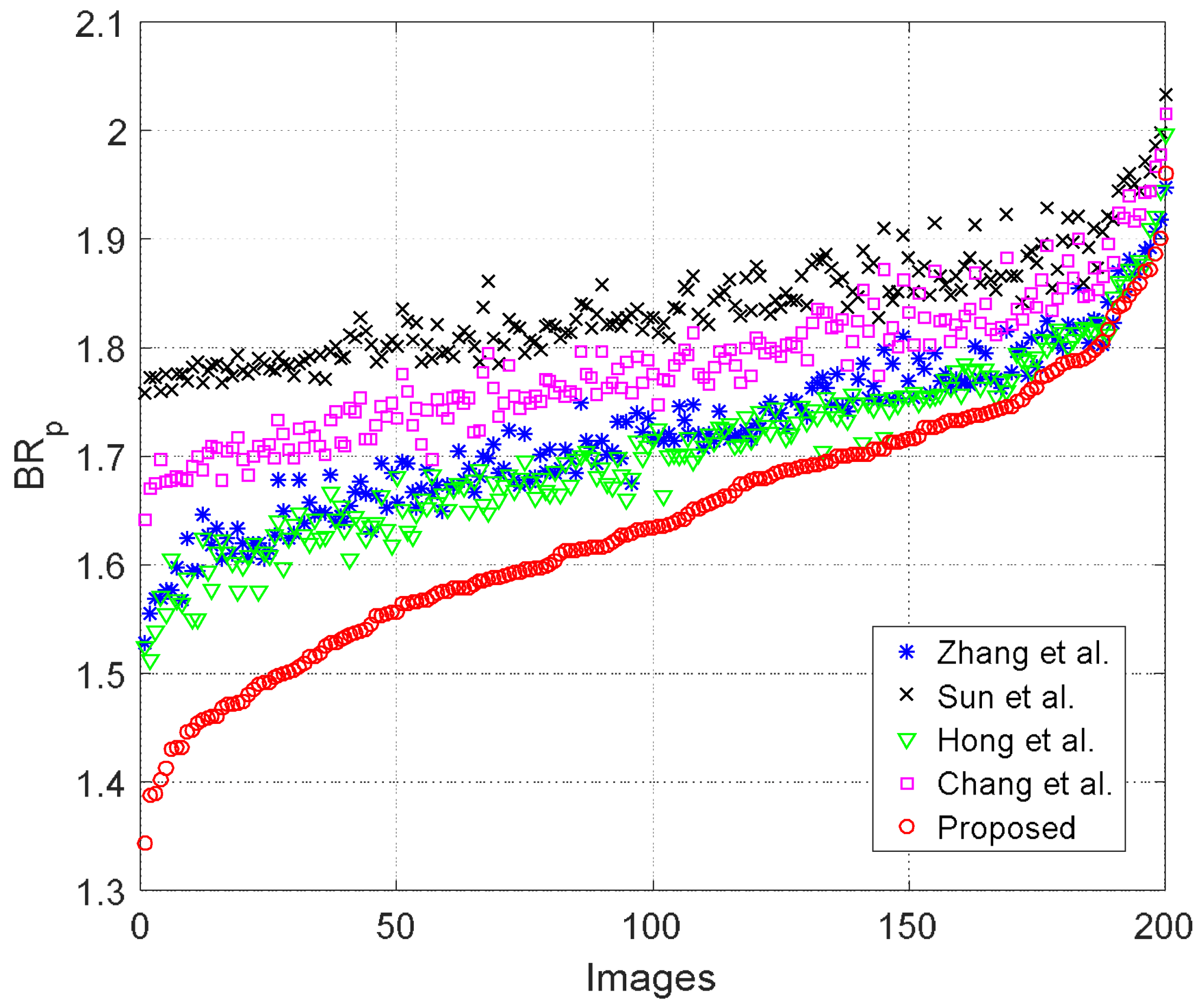
To further evaluate the performance, we also performed the test on 200 grayscale images with a size of $512\times 512$ obtained from [25]. To make a better comparison, we obtained the pure bitrate of each method, and sorted the pure bitrates obtained by the proposed method in ascending order. The bitrates of other compared methods were then rearranged using the sorted order of the proposed method. The results are shown in Figure 9.

Since the pure bitrate of a smooth image is lower than that of a complex one, we can surmise that the images on the left-hand side are smoother than the right-hand side images. As seen from Figure 9, the reduction in pure bitrate was more significant for smooth images than complex ones. Nevertheless, the proposed method offered the lowest pure bitrate for all of the 200 test images, indicating that the proposed RIT and ACC techniques are indeed more efficient than other state-of-the-art works.

5. Conclusions

In this paper, we proposed an efficient data hiding method for AMBTC compressed images. The quantization levels were first transformed into means and differences. The adaptive classification technique was then applied to classify the prediction errors into four cases with two sub-cases to efficiently encode the prediction errors. Because the classification range is determined by the distribution of prediction errors, the size of the resultant code stream was effectively reduced. The experimental results show that the proposed method not only successfully recovers the original AMBTC codes and extracts the embedded data, but also provides the lowest bitrate when compared to other state-of-the-art works.

References

- Hong, W.; Chen, T.S. A Novel Data Embedding Method Using Adaptive Pixel Pair Matching. IEEE Trans. Inf. Forensics Secur. 2012, 7, 176–184. [Google Scholar] [CrossRef]
- Liu, Y.; Chang, C.C.; Huang, P.C.; Hsu, C.Y. Efficient Information Hiding Based on Theory of Numbers. Symmetry 2018, 10, 19. [Google Scholar] [CrossRef]
- Xie, X.Z.; Lin, C.C.; Chang, C.C. Data Hiding Based on A Two-Layer Turtle Shell Matrix. Symmetry 2018, 13, 47. [Google Scholar] [CrossRef]
- Hong, W.; Chen, T.S.; Chen, J. Reversible Data Hiding Using Delaunay Triangulation and Selective Embedment. Inf. Sci. 2015, 308, 140–154. [Google Scholar] [CrossRef]
- Chen, J. A PVD-Based Data Hiding Method with Histogram Preserving Using Pixel Pair Matching. Signal Process. Image Commun. 2014, 29, 375–384. [Google Scholar] [CrossRef]
- Chen, H.; Ni, J.; Hong, W.; Chen, T.S. High-Fidelity Reversible Data Hiding Using Directionally-Enclosed Prediction. IEEE Signal Process. Lett. 2017, 24, 574–578. [Google Scholar] [CrossRef]
- Lee, C.F.; Weng, C.Y.; Chen, K.C. An Efficient Reversible Data Hiding with Reduplicated Exploiting Modification Direction Using Image Interpolation and Edge Detection. Multimedia Tools Appl. 2017, 76, 9993–10016. [Google Scholar] [CrossRef]
- Tian, J. Reversible Data Embedding Using a Difference Expansion. IEEE Trans. Circuits Syst. Video Technol. 2003, 13, 890–896. [Google Scholar] [CrossRef]
- Ni, Z.; Shi, Y.Q.; Ansari, N.; Su, W. Reversible Data Hiding. IEEE Trans. Circuits Syst. Video Technol. 2006, 16, 354–362. [Google Scholar]
- Chen, J.; Hong, W.; Chen, T.S.; Shiu, C.W. Steganography for BTC Compressed Images Using No Distortion Technique. Image Sci. J. 2010, 58, 177–185. [Google Scholar] [CrossRef]
- Chang, C.C.; Kieu, T.D.; Wu, W.C. A Lossless Data Embedding Technique by Joint Neighboring Coding. Pattern Recognit. 2009, 42, 1597–1603. [Google Scholar] [CrossRef]
- Kieu, D.; Rudder, A. A Reversible Steganographic Scheme for VQ Indices Based on Joint Neighboring and Predictive Coding. Multimedia Tools Appl. 2016, 75, 13705–13731. [Google Scholar] [CrossRef]
- Lin, C.C.; Liu, X.L.; Yuan, S.M. Reversible Data Hiding for VQ-Compressed Images Based on Search-Order Coding and Sate-Codebook Mapping. Inf. Sci. 2015, 293, 314–326. [Google Scholar] [CrossRef]
- Chang, C.C.; Liu, X.L.; Lin, C.C.; Yuan, S.M. A High-Payload Reversible Data Hiding Scheme Based on Histogram Modification in JPEG Bitstream. Imaging Sci. J. 2016, 7, 364–373. [Google Scholar]
- Hong, W. Efficient Data Hiding Based on Block Truncation Coding Using Pixel Pair Matching Technique. Symmetry 2018, 10, 36. [Google Scholar] [CrossRef]
- Zhang, Y.; Guo, S.Z.; Lu, Z.M.; Luo, H. Reversible Data Hiding for BTC-Compressed Images Based on Lossless Coding of Mean Tables. IEICE Trans. Commun. 2013, 96, 624–631. [Google Scholar] [CrossRef]
- Sun, W.; Lu, Z.M.; Wen, Y.C.; Yu, F.X.; Shen, R.J. High Performance Reversible Data Hiding for Block Truncation Coding Compressed Images. Signal Image Video Process. 2013, 7, 297–306. [Google Scholar] [CrossRef]
- Hong, W.; Ma, Y.; Wu, H.C.; Chen, T.S. An Efficient Reversible Data Hiding Method for AMBTC Compressed Images. Multimedia Tools Appl. 2017, 76, 5441–5460. [Google Scholar] [CrossRef]
- Chang, C.C.; Chen, T.S.; Wang, Y.K.; Liu, Y. A Reversible Data Hiding Scheme Based on Absolute Moment Block Truncation Coding Compression Using Exclusive OR Operator. Multimedia Tools Appl. 2018, 77, 9039–9053. [Google Scholar] [CrossRef]
- Lema, M.; Mitchell, O. Absolute Moment Block Truncation Coding and Its Application to Color Image. IEEE Trans. Commun. 1984, 32, 1148–1157. [Google Scholar] [CrossRef]
- Hong, W.; Chen, M.; Chen, T.S.; Huang, C.C. An Efficient Authentication Method for AMBTC Compressed Images Using Adaptive Pixel Pair Matching. Multimedia Tools Appl. 2018, 77, 4677–4695. [Google Scholar] [CrossRef]
- Chen, T.H.; Chang, T.C. On The Security of A BTC-Based-Compression Image Authentication Scheme. Multimedia Tools Appl. 2017, 77, 12979–12989. [Google Scholar] [CrossRef]
- Malik, A.; Sikka, G.; Verma, H.K. An AMBTC Compression Based Data Hiding Scheme Using Pixel Value Adjusting Strategy. Multidimensional Syst. Signal Process. 2017, 1–18. [Google Scholar] [CrossRef]
- The USC-SIPI Image Database. Available online: http://sipi.usc.edu/database (accessed on 29 March 2018).
- BOWS-2 Image Database. Available online: http://bows2.gipsa-lab.inpg.fr (accessed on 29 March 2018).
Figure 1.
Comparison of the distribution of prediction errors.
Figure 2.
Case classification of centralized error division (CED) and the proposed adaptive case classification (ACC).
Figure 3.
Bit-saving comparisons of the ACC and CED techniques.
Figure 4.
Quantization levels and transformed means and differences. (a) Upper quantization levels; (b) Lower quantization levels; (c) Means and (d) Differences.
Figure 5.
Six test images.
Figure 6.
Comparisons of pure bitrate under various combinations of and .
Figure 7.
The distribution of encoding cases for the Lena image.
Figure 8.
Pure bitrate comparisons of combinations of techniques.
Figure 9.
Pure bitrate comparison of 200 test images.