Probability of Conjunction Estimation for Analyzing the Electromagnetic Environment Based on a Space Object Conjunction Methodology


1
College of Information and Communications Engineering, Harbin Engineering University, Harbin 150001, China
2
College of Electronic and Information Engineering, Nanjing University of Aeronautics and Astronautics, Nanjing 211106, China
3
Department of Electrical Engineering, Comsats University Islamabad, Sahiwal Campus, Punjab 57000, Pakistan
*
Author to whom correspondence should be addressed.
Symmetry 2018, 10(7), 255; https://doi.org/10.3390/sym10070255
Submission received: 4 June 2018
/
Revised: 23 June 2018
/
Accepted: 27 June 2018
/
Published: 2 July 2018
Abstract
:The introduction of the space object conjunction method in electromagnetic compatibility modeling and simulation is quite a novel concept. It is useful for the stochastic analysis of an electromagnetic (EM) environment which is based on the probability of conjunction assessment. The space conjunction methodology is anticipated as the frontline defense for the protection of active satellites in space. EM congestion occurs in an environment with the increase in the number of operational EM devices. In a theoretical sense, this congestion is analogous to the space conjunction. Therefore, the space conjunction model can be applied in the EM scenarios. In this paper, we have investigated the application of the defined conjunction model by using the analytical expression of the probability of electromagnetic conjunction, which is based on the orbital parameters of the system under test. Additionally, we have elaborated the influence of these orbital parameters on the probability of conjunction. The simulations have been performed by considering different EM scenarios and the results are validated by using Monte Carlo simulations. The results show that errors in the analytical and Monte Carlo simulations are within a 1% range, which makes the analytical model effective. Computationally, the proposed analytical model is cost effective as compared to the numerical method, i.e., Monte Carlo. Moreover, from the results, it has been validated that the probability of conjunction increases with the increase in transmitted power and decreases with the compatible threshold limit of the receiving system, thus, making this method useful for analyzing the electromagnetic environment and as a frontline safety tool for electromagnetic systems.
1. Introduction
Radio interference has a great influence on the overall performance of wireless communication systems. Figure 1 shows the environment where different EM communication links may cause EM interferences witheach other. This has been studied for decades and spectrum management is also well in use to solve the problems of radio interference to a large extent. However, with the increase in the number of electronic transmission systems, like navigation radars, mobile stations, and smart vehicles, especially in the electronic battlefield where many communication systems are operating in considerably small areas, the performance prediction of such systems and devices nearby is still a topic of greater importance. Traditionally, the electromagnetic compatibility (EMC) evaluation of a system is done by finding the radar cross-section (RCS) and with the performance evaluation of the system under test (SUT) in the presence of electromagnetic sources in EM anechoic chambers. Probabilistic methods are also being used for electromagnetic compatibility/electromagnetic interference (EMC/EMI) evaluation in communication systems. They are primarily based on the amplitude probability distribution (APD) in which the probability of interference noise is measured as the sum of the intervals during which signal samples exceed a certain threshold, normalized by the total measurement time [1,2]. This method is quite suitable for intra-system level EMC evaluation, but for the characterization of a complete EM environment, where platforms are stationary or moving in trajectories, the prediction of the EM interference in that situation is quite complex. For inter-systems EMI evaluation, the performance of the SUT is typically predicted in the presence of EM sources, as mentioned earlier. It can be carried out in EM chambers in far-field regions, and the SUT is considered as the receiver in this evaluation [3] and [4] (pp. 1–12). For the transmitters, MIL-STD 464C [4] (pp. 14–36) and [5] regulations are applicable, in which there are defined power levels to limit its interference with other electronic devices nearby. However, these tests and measurements are carried out for static systems without considering the motion uncertainties. For moving platforms different types of uncertainties, like position, velocity, and angular uncertainties, are associated with the motion of the platform. Therefore, the main objective of this article is to analyze the EMC/EMI situation for any platform and evaluate the probability of interference among them, as it is difficult to quantify the actual strength of EMI in these situations. This is because of the behavior of EM waves in the presence of multiple sources, reflections from buildings, mountains, and terrain, is difficult to analyze. Since most of the systems/sensors are mounted on the moving platforms, this makes the situation complex enough and hard to predict with the traditional methods. Recently, Baqar et al. [6] presented an idea of EM conjunction in such scenarios and its evaluation based on the space conjunction method.
As stated earlier, the present description of radio interference needs to be updated to a more generalized version. Space conjunction, which is the first line of defense for all objects in space, is the methodology that is well being studied regarding conjunction and collision risk management of space objects [7]. This method is based on finding orbital parameters and, by using those parameters, the probability of conjunction is estimated. Space orbital conjunction methods are being used in collision detection analysis of space satellites with debris. The density of space debris is increasing with the increase in space missions. This is because some of the spacecraft and rocket bodies will fail and, hence, will not be able to leave their orbits—even if this was initially intended, as in case of Intelsat2, for example [8]. The remains resulting from such failed missions will not always naturally decay due to very little atmospheric drag that is present in some orbital regimes. Figure 2 shows the density of debris and spacecraft in orbits. The parameters, like density, speed, position, and rate of conjunction, have a greater influence on the conjunction analysis of space objects. The conjunction probability ) is the fundamental concept for the conjunction assessment and collision avoidance of space objects. The algorithms used to compute are based on state vectors of positions and velocities of the objects.
The conjunction idea can be introduced in the field of EMC/EMI modeling or predicting. In the EMC/EMI model, the platforms can be airplanes, ships, and cars, which are all moving in their own trajectories, called their orbits. If a radiation source on one platform has some interference on any devices on other platforms, it can be considered as a conjunction in the sense of electromagnetics. The method to judge whether the EM conjunction has happened or not, we usually adopt the concept of space debris as EM congestion. If talking particularly in terms of dense electromagnetic scenarios, like in electronic warfare, where many tactical movements are going on, all systems remain in some orbits (trajectories) and have associated orbital parameters (orbital parameters details are discussed in next section). An overview of the orbital parameters and their influence on the orbital conjunction analysis for EMC/EMI evaluation is given by Baqar et al. [6]. If information of the radiation source is given, its interference orbit can be found. When all orbital parameters of interference sources are known, it is not so difficult to predict the conjunction of two radio systems. The predicted results will help in analyzing the EM situation. This helps in taking precautionary measures for avoiding EM interference, hence resulting in improving the effectiveness of the systems. Since all platforms are well equipped with sophisticated EM sensors, this makes the environment electromagnetically dense. The increase of commercial platforms, like airplanes, cargo ships, and mobile stations, make the EM environment even more congested. The overview of such an EM-dense scenario, where multiple platforms are moving in their respective orbits and having particular EM power contours, can be seen in Figure 3. The power distribution of these EM sources is analogous to the size of space objects and the rate of EM conjunction can be treated as the rate of space conjunction. Based on these analogies, we can presume that the protection methods used in space conjunction can also be applied in electromagnetic situations, which gives a better situational analysis of the scenario. This paper is organized as follows: Section 2 gives the details of the conjunction prediction method; Section 3 describes the probability of the EM conjunction estimation; Section 4 shows the associated simulation results; Section 5 presents the discussion; and Section 6 offers conclusions and related future work.
2. Conjunction Prediction
For the conjunction prediction of any device or system, it is important to know the concept of the orbit and its associated parameters, these parameters will be called orbital parameters later in this article. The orbital parameters for the EM scenario can be written as . These parameters are —system’s position, —the time of operation,—operational frequency, —power density, and —spatial coverage (directional or omnidirectional). How are these parameters expressed for finding ? This is a question of interest. In this paper, we attempt to formulate an analytical expression of based on these orbital parameters. It is not easy to find the exact numerical solution. However, it is possible to approximate the solution and obtain the results within error limits. Conjunction assessment and its avoidance is of great importance considering in space or EMC/EMI conjunctions. For defining conjunction, we first consider the physical trajectory of the system and find the expression of . Then we apply a radio propagation model for complete elaboration of . While considering the trajectory of the system, the description of for such a scenario is defined as follows: the state vector (position and velocity) of system 1 () is with the covariance matrix . It is assumed that at the state and covariance matrix is known for . is the time of closest approach where the conjunction is likely to occur. Similarly, for system 2 (), the state and covariance vectors, and are known at . By using the closest approach analysis, at the time of closest approach (), corresponding state and covariance matrices are, , (τ), and (τ), respectively. The safety radii of the two systems are and , respectively. This is illustrated in Figure 4 which shows the positioning error ellipsoid in the trajectory and associated state parameters at the initial and closest approach times. All of these above parameters are used to compute , which is considered as a significant parameter in finding the occurrence of conjunction. The trajectory estimation model and the covariance must be computed accurately as it may cause false alarms in the calculation.
3. Analytical Expression of the Probability of EM Conjunction
In this section, we will derive an analytical expression for . We start by defining the conjunction definition for two objects and compute the probability of conjunction , and then modify the parameters for finding the . There are various methods to calculate the probability of conjunction given by [9,10,11,12]. In this article, we used the method given by Chan [9] and Alfano et al. [11], due to its accuracy and less computational cost. As discussed in Section 2, if the state covariance matrix is given at each instance and is assumed to be statistically independent then we can combine the covariance matrix [9]. If is the combined covariance matrix, then the probability density function (PDF) for the relative position between the both objects will be as follows [13]:
where:
Therefore, the probability of conjunction ( at any instant of time is defined as:
where is the volume of the overlap region of the distributions. For simplification, let us assume both objects are spheres with as the total safety radius i.e., , then the volume , swept by the sphere centered at the primary (origin) is given as:
The closed form solution for the above 3-D integral is difficult to find. Chan [9] modified the integral to 2-D by taking the following assumptions: the relative velocity of two space objects are very high and they contribute to much less time in the conjunction instance, so the relative velocity can be assumed rectilinear. He then further reduced the integral to an isotropic distribution for which it is easy to obtain the solution via numerical expansion. Alfano, in [14], said that the same 3-D to 2-D integral transformation can be directly used in 2-D problems without any approximation. Therefore, EMC evaluation for moving platforms, and considering most of the platforms in the real-world as 2-D, we consider only 2-D cases in this paper and derive the expression of .
The joint PDF of the relative position coordinates (assumed uncorrelated) for the two objects (primary and secondary objects) will be bivariate Gaussian. If they are correlated, then the transformation of the principal axis can be applied [9]. can be defined as the surface integral of a bivariate PDF which is centered at , and has a combined standard deviations in and as and , respectively. The surface integral is over a circular cross-section area of combined radius , as shown in Figure 5. The integral parameters on the conjunction plane are,,, , and. The can be written mathematically as the total area laying inside the circular cross-section:
Chan [9] and Xian et al. [15] presented an improved analytical expression for computing by solving and replacing the two-dimensional integral by a one-dimensional Rician PDF, which can be evaluated in the form of a convergent infinite series. Chen [7] did the analogous work in which he presented the first term and the recursive expression of the infinite series, which is helpful for the programing of analytical expression due to its simplification.
The variables in Equation (3) can be parameterized as:
by integration of over a circular region from 0 to 2π, the 2-D integral is converted to 1-D. After some mathematical simplification, Pc is given as:
where is the modified Bessel function. This PDF arises in most signal detection problems. The transformation was obtained by Rice [16], hence, it is called Rician PDF. The solution for the above Bessel function can be written as an infinite convergent series:
Therefore:
We can write:
where:
The first term in the series is:
By integration and simplification, we have:
Substituting :
Assuming and z as dimensionless quantities as:
The expression in Equation (12) reduces to:
The and terms can be expressed recursively as:
Defining a new variable as:
Therefore, the recursive expression of Equation (14) can be written as:
Thus, any term of can be obtained from the above recursive expression for all . To approximate it, let us assume first that terms can give , the probability of conjunction, so we may write:
Xian et al. [11] state that in conjunction analysis of space objects, where is considered relatively smaller than the position uncertainties and , then the truncation error is reduced to if considered only the first term as . The truncation error is reduced further to if the first two terms are considered. Thus, the higher sums contribute a negligible difference in summation of . Therefore, considering only the first term yields the error in the 3rd significant digit. By substituting the values of and in Equation (13), the estimated analytical expression of is obtained as:
where is the total size of the objects i.e., the size of transmitter and receiver systems, and is given as:
and are the diagonal elements of the combined covariance matrix, which is:
and are the difference of the mean trajectory paths of the two platforms, i.e.,:
Although Equation (18) serves as the basic formula to analyze the probability of conjunction, if the cross-sectional radius and the miss distance is greater than or , then one might have to consider more terms to compute accurately [7]. Since is the total size of the conjunction radius, for EM systems, considering an isotropic antenna, the propagation distance is analogous to the radius of the object. In this case, calculations by using Equation (17) will give accurate results as in the EMC scenario is usually greater (depending upon the operating frequency) than or We may write, the size of the transmitter, as a maximum of physical and EM size, i.e.,:
Since we are concerned with the EM conjunction, therefore, Equation (19) becomes:
where and are the EM sizes of the transmitter and receiver, respectively. For EMC evaluation, the receiver, which is the system under test, has its own compatibility threshold and is considered passive during the testing. This makes the, Therefore, the conjunction probability in Equation (18) can be written as:
The size depends on the compatibility threshold limit (of the receiver [5]. is the maximum threshold for any electronic system at which it remains electromagnetically compatible. We can find by using Friis Equation, considering free space path loss [17]:
where is the transmitted power, is the threshold limit of the system under test (SUT- receiver), are the antenna gains of the transmitter and the receiver, respectively, is the operating frequency, and is the velocity of electromagnetic waves.
Considering the scenario where both platforms have transmitting systems installed, then of system 1 depends on (the threshold of receiver system 2). Similarly, theof system 2 is associated with and can be calculated by using Equation (26). Therefore, having and as their respective probabilities of conjunction, as shown in the schematic in Figure 6, the total probability of conjunction ( can be realized as a parallel system scenario. Therefore, from the theory of reliability, the total probability of conjunction in terms of an individual system probability [18] can be written as:
Using the complementary approach, we can write:
For a transceiver case the transmitter and the receiver systems are independent of each other, therefore:
Equation (27) is the analytical expression of total for the scenario where both platforms have transmitters. The EM size depends on the threshold limit of system 2 while the EM size used for expression depends on the threshold value of system 1.
4. Simulation Results
For the simulations, we consider two platforms, assuming transmitter (a radar system) on one platform and the receiver on the other. Both systems are installed on a platform having rectilinear motion and moving in a trajectory that has random perturbations in the and coordinates. We assume the perturbations are due to external factors, like weather, turbulence, and efficiency of the positioning devices, hence, causing random errors in the positioning of the platforms/systems since, for an unbiased estimator, the root mean square error (RMSE) is the standard deviation [19]. Horizontal positioning accuracy of a GPS systems is normally within the range of 28 [20], so the mean square error would be in the range of 4–64 m2. In all simulations, we take the variance from this range. We further assumed the positioning errors in and are uncorrelated, i.e., = 0, having a mean value equal to zero. Both antennas are assumed to be omnidirectional with unity gains. Since navigational radars are operating at high frequency, mainly in we assume the frequency of operation is 8 . Due to the high power of the radars, transmitted power is taken from the range 60–66 dBm, while the threshold of ( is taken from 0–10 dBm, which is the upper limit assumed for impeccable and linear functionality of the system. This range threshold is taken as microware amplifiers in EM receivers usually get saturated at these values, however, this threshold limit can be adjusted depending upon the type of EMI evaluation to be performed, e.g., EM interference from a jamming perspective, saturation, or burnout, etc. To compute the probability of EM conjunction, we neglect the effect of the physical size of the platforms. We further assumed that both platforms are moving with the same velocity. These initial conditions are applied in all simulations. Simulations are performed for three different trajectories. All three scenarios are shown in Figure 7, Figure 8 and Figure 9. First is the straight-line scenario where systems are moving close and crossing each other, second case is of a circular trajectory (tangent) scenario in which they make a tangent at the time of closest approach. The third case is also circular trajectory (crossing) scenario, but moving close and crossing each other at two different instances. is computed for all simulation scenarios by using Equation (17), written , and the results are validated with Monte Carlo simulations, and written as .
5. Discussions
The analytical expression of shows that it depends on the four orbital parameters, e.g., position coordinates (trajectory mean), error covariance, transmitted power, and receiver threshold. Therefore, simulations are conducted in four groups and the results are compiled to see the effect of trajectory, transmitted power , receiver threshold , and position covariance on . The effect of trajectory is shown in Figure 10, Figure 11 and Figure 12, while the rest of the results are organized in Table 1, Table 2 and Table 3.
Figure 10, Figure 11 and Figure 12 show the effect of trajectories on the . In all three trajectories, all variables are kept as mean: = 0, variance: = 10 , cov: = 0, = , and = . In a straight line trajectory, Figure 10, it can be seen that is increasing as both platforms are approaching close to each other. The number of peaks are also significant as it gives the number of instances at which systems are in relatively EMC incompatible zones. In Figure 10 only one peak exists for a small duration. This means that, in the whole trajectory, there exists only a single instance of closest approach where conjunction probability is high. The width of the peak shows the duration for which is subjected to the relatively high power in the whole trajectory. In Figure 11, the duration of is greater as the platforms are in close vicinity to each other for a longer duration (making tangent). In Figure 12, there are two closest approach instances , which shows there are two possible instances of EM conjunction in that trajectory.
For all three trajectories, the effects of , , and the position error variance on are simulated and the results are arranged in Table 1, Table 2 and Table 3. The maximum value of is taken at the time of closest approach (). Simulations are done with initial conditions of position uncertainty as mean: = 0, variance: = 10 , cov: = 0. For analyzing the effect of , we keep fixed at 10 . from the Monte Carlo simulation and analytical method, at the time of closest approach, is shown in Table 1. We can see that has a direct relation with (Figure 13a), which means as the transmitter power is increased, the probability of conjunction is also increased, which validates the concept of EMI in any electronic system. The percentage error in between simulated and analytical methods at the time of closest approach is calculated in the last column, showing the effectiveness of the analytical method.
Keeping the same position uncertainty values and fixed at , the effect of is summarized in Table 2. It can be seen that the increase in the compatibility threshold of the receiver system results in the deterioration of the probability of conjunction exponentially (Figure 13b), hence, making the system more likely EM compatible.
Finally, to see the effect of variance on , we keep and of the systems fixed at and , respectively. The results in Table 3 show the inverse relation of variance with . This is because, if perturbations are high, there is a more likely chance to miss the collision. These results are useful in predicting the EM environment. By applying the threshold limit on , we can set different electromagnetic compatible levels in the whole trajectory of any platform.
The computational resources used in terms of average time is also computed for both simulation methods (simulation resources used: processor: Intel (R) Core™ i3 CPU M380 @ 2.53 GHz; RAM: 8 GB; OS type: Windows 64-bit; MATLAB, Version 9.4.0.813654 (R2018a), 64-bit). Each trajectory scenario consists of 2000 samples. The Monte Carlo simulation with 50,000 points is performed at each sample of a trajectory. The average time consumed for the Monte Carlo simulation is , while using analytical Equation (17) with , the average time is reduced to only .
6. Conclusions
Space orbital conjunction analysis is one of the critical aspects in orbital conjunctions. As the EM environment is also becoming dense, the concept of space orbital conjunction is quite appealing to cope with EMC/EMI problems. The space conjunction method based on the probability of conjunction estimation is applied, and the orbital parameters are modified according to the EMI scenario. By knowing the prior information of the trajectory, error covariance matrix, and the specifications of transmitter and receiver systems, theanalysis can give the EMC compatibility of the systems on the platform in a specific trajectory. The results based on the analytical expression of are validated by using Monte Carlo simulations. The percentage errors between Monte Carlo and analytical expressions lie within a 1% range, which authenticates the effectiveness of the proposed analytical expression with less computational cost. The method is of great importance and well suited for moving platforms to analyze the electromagnetic compatibility in their orbit. However, the proposed model is limited to 2-D scenarios and considering omnidirectional transmitters only, i.e., making the EM shape spherical or circular (considering a 2-D or 3-D antenna pattern). These limitations simplify the calculations, but decrease their accuracy when quantifying the level of EMI. The analysis is also significant in a way that we can set the protection threshold to take precautionary measures for the safety of onboard electronic devices. Moreover, for all transmitters () in a vicinity, conjunction probabilities can be computed and, based on the protection threshold limit, it is easy to indicate the trajectory or path which is considered more EM compatible. Additionally, this method is of key importance in electronic warfare scenarios, where different platforms are moving in a close vicinity creating more chances of interference among them. Since the current proposed model has some limitations that are mentioned above, for future work we will try to investigate those limitations to make the model robust for any real-time situations (2-D or 3-D). In the future, we will also try to perform a sensitivity analysis of the parameters that are used in the conjunction model.
Author Contributions
All the authors contributed equally to the work. All authors have read and approved the final manuscript.
Funding
This research was funded by the International Exchange Program of Harbin Engineering University for Innovation-oriented Talents Cultivation. This work was partially supported by the National Key Research and Development Program of China (2016YFE0111100), the Key Research and Development Program of Heilongjiang (GX17A016), the Science and Technology innovative Talents Foundation of Harbin (2016RAXXJ044), the Natural Science Foundation of Beijing (4182077), and the China Postdoctoral Science Foundation (2017M620918).
Conflicts of Interest
The authors declare no conflict of interest.
References
- Matsumoto, Y.; Wiklundh, K. Evaluation of impact on digital radio systems by measuring amplitude probability distribution of interfering noise. IEICE Trans. Commun. 2015, 98, 1143–1155. [Google Scholar] [CrossRef]
- Rahman, M.J.; Wang, X. Probabilistic analysis of mutual interference in cognitive radio communications. In Proceedings of the IEEE Global Telecommunications Conference, Kathmandu, Nepal, 5–9 December 2011; pp. 1–5. [Google Scholar]
- Violette, N.J.L.; White, D.R.J. Electromagnetic Compatibility Handbook, 1st ed.; Springer: New York, NY, USA, 1987; pp. 106–146. [Google Scholar]
- Morgan, D. A Handbook for EMC Testing and Measurement, 2nd ed.; The Institution of Engineering and Technology: London, UK, 2007; pp. 1–12, 14–36. [Google Scholar]
- Department of Defense USA. MIL-STD-464C, USA, 1 December 2010. Available online: http://everyspec.com/MIL-STD/MIL-STD-0300-0499/MIL-STD-464C_28312/ (accessed on 1 December 2010).
- Baqar, A.H.; Xu, P.; Tao, J.; Zhang, Y.C. Application of space object conjunction method in the system level EMC evaluation. In Proceedings of the Asia-Pacific International Symposium on Electromagnetic Compatibility, Seoul, Korea, 20–23 June 2017; pp. 253–255. [Google Scholar]
- Lei, C.; Xian, Z.B.; Yan, G.L.; Ke, B.L. Orbital Data Applications for Space Objects, 1st ed.; Springer: Singapore, 2017. [Google Scholar]
- Anselmo, L.; Pardini, C. The end-of-life disposal of the Italian geostationary satellites. Adv. Space Res. 2014, 34, 1203–1208. [Google Scholar] [CrossRef]
- Chan, K. International Space Station Collision Probability; The Aerospace Corporation: Chantilly, VA, USA, 1997; Available online: http://aero.tamu.edu/sites/default/files/faculty/alfriend/S4.2%20Chan.pdf (accessed on 1 June 2018).
- Xiao, L.X.; Xiong, Y.Q. A method for calculating probability of collision between space objects. Res. Astron. Astrophys. 2014, 14, 601–609. [Google Scholar] [Green Version]
- Alfano, S.; Oltrogge, D. Probability of Collision: Valuation, variability, visualization, and validity. In Proceedings of the AIAA/AAS Astrodynamics Specialist Conference, Long Beach, CA, USA, 13–16 September 2016; p. 5654. [Google Scholar]
- Patera, R.P. A general method for calculating satellite collision probability. J. Guidance Control Dyn. 2001, 24, 716–722. [Google Scholar] [CrossRef]
- Papoulis, A. Probability, Random Variables, and Stochastic Processes, 3rd ed.; McGraw-Hill: New York, NY, USA, 1991. [Google Scholar]
- Alfano, S. Review of conjunction probability methods for short-term encounters. Adv. Astronaut. Sci. 2007, 127, 719–746. [Google Scholar]
- Bai, X.Z.; Chen, L. A Rapid Algorithm of Space Debris Collision Probability Based on Space Compression and Infinite Series. Acta Math. Appl. Sin. 2009, 32, 336–353. [Google Scholar]
- Rice, S.O. Mathematical Analysis of Random Noise. Bell Syst. Tech. J. 1944, 23, 282–332. [Google Scholar] [CrossRef]
- Shaw, J.A. Radiometry and the Friis transmission equation. Am. J. Phys. 2013, 81, 33–37. [Google Scholar] [CrossRef]
- Romeu, J.L. Understanding Series and Parallel Systems Reliability; Department of Defense, Reliability Analysis Center: Rome, NY, USA, 2004; Volume 11, 8p. [Google Scholar]
- Willmott, C.J.; Matsuura, K. On the use of dimensioned measured of error to evaluate the performance of spatial interpolators. Int. J. Geogr. Inf. Sci. 2006, 20, 89–102. [Google Scholar] [CrossRef]
- Hughes, W.J. Global Positioning System (GPS) Standard Positioning Service (SPS) Performance Analysis Report; Federal Aviation Administration, GPS Product Team: Washington, DC, UK, 2014. Available online: http://www.nstb.tc.faa.gov/reports/PAN96_0117.pdf (accessed on 1 June 2010).
Figure 1.
Communication link and electromagnetic interference sources (courtesy image: Navy continues electronic warfare upgrades for ships, by Kevin Mccaney, 2016).
Figure 1.
Communication link and electromagnetic interference sources (courtesy image: Navy continues electronic warfare upgrades for ships, by Kevin Mccaney, 2016).

Figure 2.
Simulation of debris pattern orbiting around Earth (courtesy image: created by the Institute of Aerospace Systems at the Technische Universität Braunschweig Germany, 2015).
Figure 2.
Simulation of debris pattern orbiting around Earth (courtesy image: created by the Institute of Aerospace Systems at the Technische Universität Braunschweig Germany, 2015).

Figure 3.
EM conjunction scenario (platforms with orbits and associated EM size).

Figure 4.
Conjunction behavior in describing .

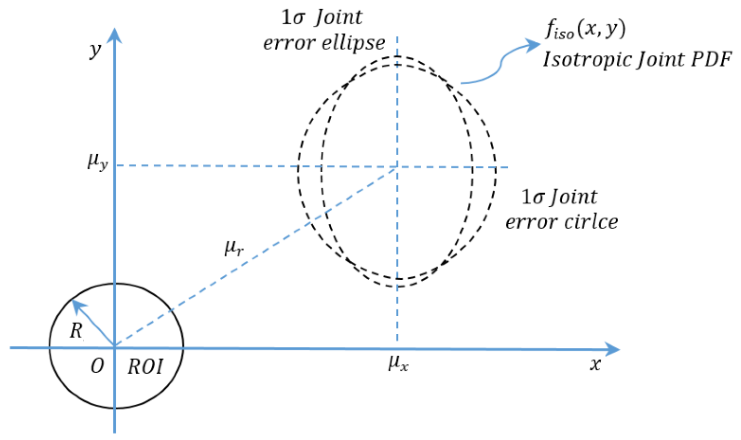
Figure 5.
Parameters of : probability density function and radius of conjunctional cross-section area.
Figure 5.
Parameters of : probability density function and radius of conjunctional cross-section area.

Figure 6.
Transceiver scenario.

Figure 7.
Straight line trajectory: ; ; error parameters: mean:, variance: 10, cov: .

Figure 8.
Circular trajectory (tangent): ; ; error parameters: mean:, variance: 10, cov: .

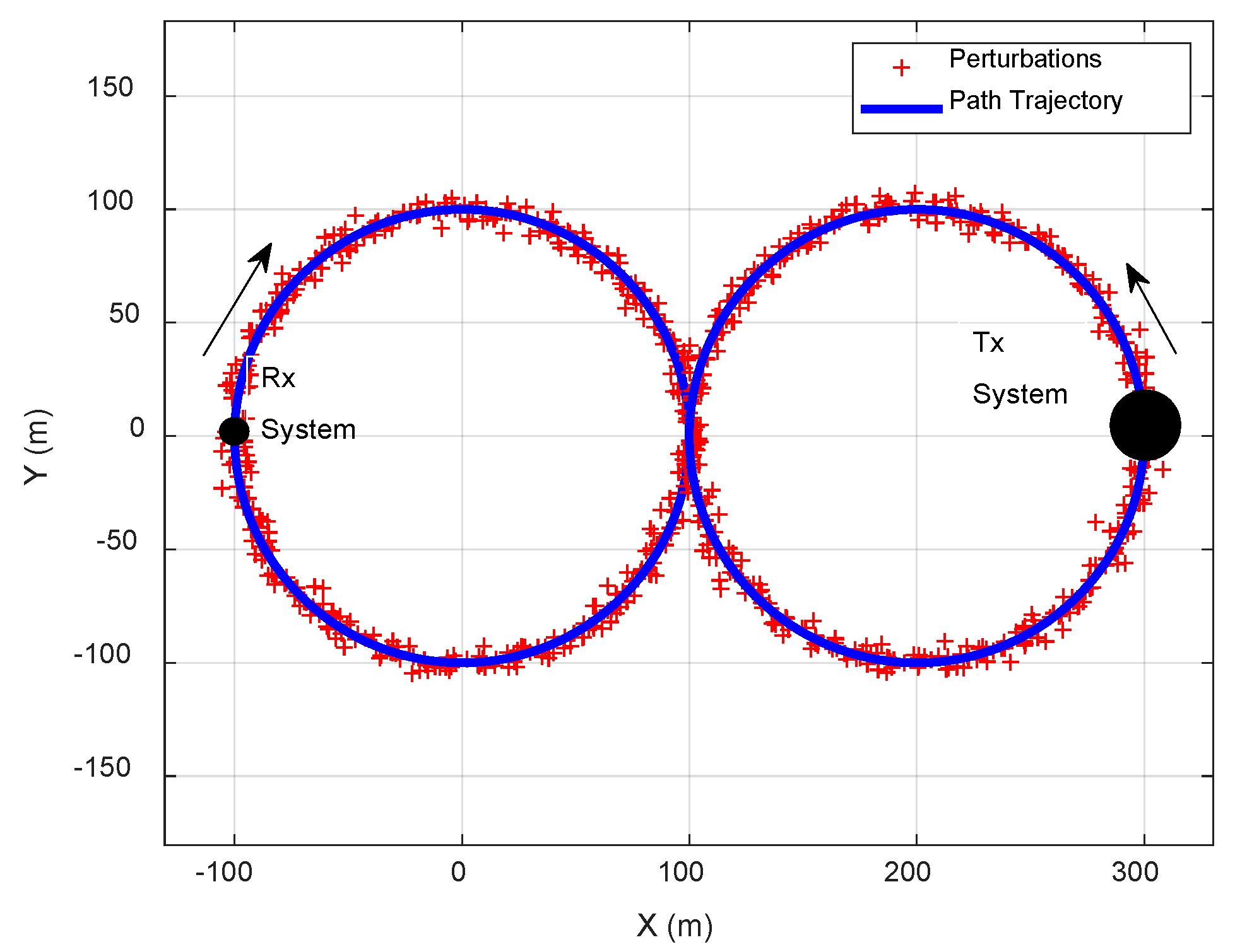
Figure 9.
Circular trajectory (Crossing): ; ; error parameters: mean:, variance: 10, cov: .

Figure 10.
and error in (Monte Carlo and Analytical) for straight line trajectory; ; ; error parameters: mean:, variance: 10 , cov: .
Figure 10.
and error in (Monte Carlo and Analytical) for straight line trajectory; ; ; error parameters: mean:, variance: 10 , cov: .

Figure 11.
and error in (Monte Carlo and Analytical) for circular trajectory (tangent); ; ; error parameters: mean:, variance: 10 , cov: .
Figure 11.
and error in (Monte Carlo and Analytical) for circular trajectory (tangent); ; ; error parameters: mean:, variance: 10 , cov: .

Figure 12.
and error in (Monte Carlo and Analytical) for circular trajectory (crossing); ; ; error parameters: mean:, variance: 10 , cov: .
Figure 12.
and error in (Monte Carlo and Analytical) for circular trajectory (crossing); ; ; error parameters: mean:, variance: 10 , cov: .

Figure 13.
(a) Effect of on ; (b) Effect of on ; (c) variance on.


Table 1.
Effect of transmitted power on ; position uncertainty (mean: = 0, variance: = 10 , cov: = 0).
Table 1.
Effect of transmitted power on ; position uncertainty (mean: = 0, variance: = 10 , cov: = 0).
| Trajectory Type | Transmitter Power | Receiver Threshold | Max. Probability of Interference Monte Carlo at | Max. Probability of Interference Analytical at | % Error in at |
|---|---|---|---|---|---|
| Straight line Figure 7 | 60 | 10 | 0.0221 | 0.0200 | 0.5362 |
| 63 | 0.0436 | 0.0435 | 0.1813 | ||
| 66 | 0.0846 | 0.0847 | 0.1412 | ||
| Circular Tangent Figure 8 | 60 | 10 | 0.0221 | 0.0220 | 0.2773 |
| 63 | 0.0436 | 0.0436 | 0.0765 | ||
| 66 | 0.0851 | 0.0848 | 0.3691 | ||
| Circular Crossing Figure 9 | 60 | 10 | 0.0220, 0.0222 | 0.0219, 0.0220 | 0.2140, 0.7585 |
| 63 | 0.0437, 0.0435 | 0.0434, 0.0434 | 0.5892, 0.3119 | ||
| 66 | 0.0850, 0.0848 | 0.0848, 0.0848 | 0.2381, −0.0012 |
Table 2.
Effect of Receiver’s threshold on ; position uncertainty (mean: = 0, variance: = 10 , cov: = 0).
Table 2.
Effect of Receiver’s threshold on ; position uncertainty (mean: = 0, variance: = 10 , cov: = 0).
| Trajectory Type | Receiver Threshold | Transmitter Power | Max. Probability of Interference— Monte Carlo at | Max. Probability of Interference— Analytical at | % Error in at |
|---|---|---|---|---|---|
| Straight line | 0 | 60 | 0.2014 | 0.1996 | 0.9233 |
| 1 | 0.1625 | 0.1621 | 0.2439 | ||
| 3 | 0.1054 | 0.1052 | 0.2259 | ||
| 5 | 0.0682 | 0.0679 | 0.3717 | ||
| 7 | 0.0435 | 0.0433 | 0.3933 | ||
| 9 | 0.0278 | 0.0276 | 0.5632 | ||
| 10 | 0.0221 | 0.0220 | 0.5362 | ||
| Circular Tangent | 0 | 60 | 0.1996 | 0.1995 | 0.0711 |
| 1 | 0.1630 | 0.1619 | 0.6292 | ||
| 3 | 0.1060 | 0.1056 | 0.3603 | ||
| 5 | 0.0680 | 0.0680 | −0.0158 | ||
| 7 | 0.0435 | 0.0434 | 0.2033 | ||
| 9 | 0.0277 | 0.0276 | 0.2671 | ||
| 10 | 0.0221 | 0.0220 | 0.2773 | ||
| Circular Crossing | 0 | 60 | 0.1989, 0.1996 | 0.1990, 0.1990 | −0.0313, 0.2789 |
| 1 | 0.1619, 0.1631 | 0.1620, 0.1620 | −0.0140, 0.7323 | ||
| 3 | 0.1056, 0.1055 | 0.1055, 0.1055 | 0.0724, −0.0336 | ||
| 5 | 0.0682, 0.0679 | 0.0679, 0.0679 | 0.4257, −0.0283 | ||
| 7 | 0.0435, 0.0434 | 0.0434, 0.0433 | 0.1440, 0.1134 | ||
| 9 | 0.0277, 0.0275 | 0.0276, 0.0275 | 0.4398, −0.1769 | ||
| 10 | 0.0220, 0.0222 | 0.0219, 0.0220 | 0.2141, 0.7585 |
Table 3.
Effect of variance on ; position uncertainty (mean: = 0, cov: = 0).
| Trajectory Type | Position Variance ) | Transmitter Power | Receiver Threshold | Max. Probability of Interference Monte Carlo at | Max. Probability of Interference Analytical at | % Error in at |
|---|---|---|---|---|---|---|
| Straight line | 10 | 60 | 10 | 0.0221 | 0.0220 | 0.5362 |
| 35 | 0.0064 | 0.0063 | 0.8982 | |||
| 50 | 0.0045 | 0.0044 | 0.6667 | |||
| 64 | 0.0035 | 0.0035 | 0.9443 | |||
| Circular Tangent | 10 | 60 | 10 | 0.0221 | 0.0220 | 0.2773 |
| 35 | 0.0064 | 0.0063 | 0.6218 | |||
| 50 | 0.0045 | 0.0044 | 0.7721 | |||
| 64 | 0.0035 | 0.0035 | 0.9169 | |||
| Circular Crossing | 10 | 60 | 10 | 0.0220, 0.0222 | 0.0219, 0.0220 | 0.2141, 0.7585 |
| 35 | 0.0064, 0.0064 | 0.0063, 0.0063 | 1.1322, 1.3058 | |||
| 50 | 0.0045, 0.0045 | 0.0044, 0.0044 | 0.8144, 1.2290 | |||
| 64 | 0.0035, 0.0035 | 0.0035, 0.0035 | 0.5313, 0.9591 |
© 2018 by the authors. Licensee MDPI, Basel, Switzerland. This article is an open access article distributed under the terms and conditions of the Creative Commons Attribution (CC BY) license (http://creativecommons.org/licenses/by/4.0/).
Share and Cite
MDPI and ACS Style
Baqar, A.H.; Jiang, T.; Hussain, I.; Farid, G. Probability of Conjunction Estimation for Analyzing the Electromagnetic Environment Based on a Space Object Conjunction Methodology. Symmetry 2018, 10, 255. https://doi.org/10.3390/sym10070255
AMA Style
Baqar AH, Jiang T, Hussain I, Farid G. Probability of Conjunction Estimation for Analyzing the Electromagnetic Environment Based on a Space Object Conjunction Methodology. Symmetry. 2018; 10(7):255. https://doi.org/10.3390/sym10070255
Chicago/Turabian StyleBaqar, Asad Husnain, Tao Jiang, Ishfaq Hussain, and Ghulam Farid. 2018. "Probability of Conjunction Estimation for Analyzing the Electromagnetic Environment Based on a Space Object Conjunction Methodology" Symmetry 10, no. 7: 255. https://doi.org/10.3390/sym10070255
Note that from the first issue of 2016, this journal uses article numbers instead of page numbers. See further details here.