A Modified Dolph-Chebyshev Type II Function Matched Filter for Retinal Vessels Segmentation

Abstract

In this paper, we present a new unsupervised algorithm for retinal vessels segmentation. The algorithm utilizes a directionally sensitive matched filter bank using a modified Dolph-Chebyshev type II basis function and a new method to combine the matched filter bank’s responses. Fundus images from the DRIVE and STARE databases, as well as high-resolution fundus images from the HRF database, are utilized to validate the proposed algorithm. The results that we achieve on the three databases (DRIVE: Sensitivity = 0.748, F1-score = 0.786, G-score = 0.856, Matthews Correlation Coefficient = 0.758; STARE: Sensitivity = 0.793, F1-score = 0.780, G-score = 0.877, Matthews Correlation Coefficient = 0.756; HRF: Sensitivity = 0.804, F1-score = 0.764, G-score = 0.883, Matthews Correlation Coefficient = 0.741) are higher than many other competing methods.

1. Introduction

Retinal blood vessels analysis is beneficial for a non-invasive detection of several eye-related diseases, such as diabetic retinopathy, hypertension and vein occlusion [1]. Such analysis requires segmented retinal blood vessels which are commonly provided by ophthalmologists. However, the ophthalmologist usually performs retinal vessels segmentation manually. This manual segmentation is prone to errors and is time-consuming, particularly for blood vessels with complicated structures. Hence, it is worthwhile to construct an automatic and robust algorithm for retinal vessels segmentation.

Several algorithms of retinal vessels segmentation have been developed to assist ophthalmologists in assessing retinal vessels’ locations. The methods can be divided into two classes, viz. unsupervised and supervised approaches. Unsupervised approaches which include filter-based [2,3,4,5], tracking-based [6] and iterative-based [7,8] methods perform retinal vessel segmentation by either locally or entirely approximating retinal vessels pixels without any prior knowledge and labeled ground truth. On the contrary, given a set of features vectors and labeled ground truths, several supervised classifiers such as Gaussian Mixture Model [9,10,11], cross-modality learning [12], support vector machine [13] and convolutional neural networks [14,15,16] map fundus image pixels into a vessel or non-vessel class.

Most of the existing unsupervised methods are unable to provide desired results on some challenging situations, such as segmenting thin vessels and detecting vessels in the presence of pathologies [4]. These pathologies are commonly the diabetic retinopathy landmarks, which include bright lesions (exudates or cotton wall spots) and dark lesions (microaneurysms or hemorrhages) [7]. On the contrary, although supervised methods usually offer more reliable vessels segmentation results, they typically require a large number of training samples and are prone to heavy computational complexities. In addition to those drawbacks, most existing methods are only developed and evaluated using low-resolution fundus images from the DRIVE [6] and STARE [17] databases. Although some methods such as those in [3,5,13,16] have been developed using high-resolution fundus images, these methods are not able to achieve similar superior performance for high-resolution fundus images as achieved on low-resolution fundus images. Given high-resolution images will be more useful for evaluation of blood vessels segmentation methods [3], there is a need to further improve the methods such that they can perform as well or better for high-resolution images.

In this paper, we propose a new algorithm for retinal vessels segmentation. The algorithm includes a novel multi-scale and orientation matched filter bank using a modified Dolph-Chebyshev type II basis function (MDCF-II) and a new method to incorporate the matched filter bank’s responses. In addition, it is also shown that MDCF-II with an appropriate scale is the most suitable model for retinal vessels with thin, medium and thick widths. Hence, the multi-scale concept used in this paper allows the matched filters to detect retinal vessels in all possible widths. The proposed algorithm is evaluated using the 40 low-resolution images from the DRIVE [6] and STARE [17] databases and 45 high-resolution images from the HRF database [3]. Specifically, quantitative measures such as sensitivity $(Se)$, specificity $(Sp)$, positive predictive value $(Ppv)$, F-1 score $(F1)$, G-mean $(G)$ and Matthews correlation coefficient $(MCC)$ are used for performance evaluation. In the experiment, the proposed algorithm is able to achieve the best value for $Se$, $F1$, G and $MCC$ among all competing methods on the high-resolution fundus images.

The rest of the paper is organized as follows. Section 2 describes the concept of our new matched filter bank together with the correlation measures of MDCF-II. The correlation is done with respect to some intensity profiles of retinal vessels’ cross sections and compared to the conventional matched filter’s basis functions. Section 3 elaborates the details of our algorithm along with the parameters setting procedures. Some results of our algorithm along with the comprehensive discussion are presented in Section 4. Section 5 provides the performance measure of the proposed algorithm and comparison to other existing methods as well as the effect of the parameter to the proposed algorithm performance. Finally, the research work is summarized in Section 6.

2. Design of the New Matched Filter Window

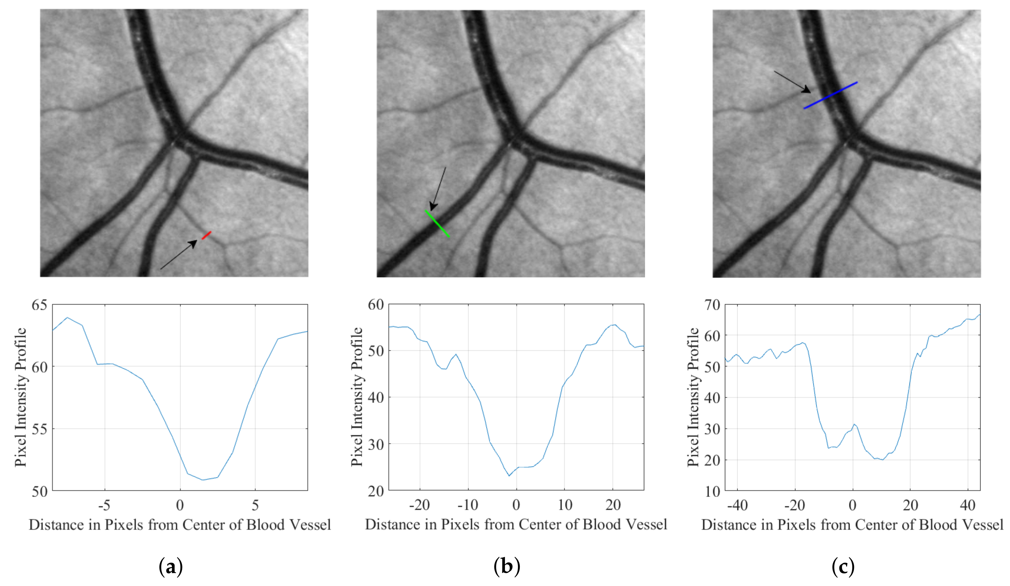
The idea of using a matched filter to detect retinal vessels is basically finding and designing a suitable model for intensity profiles of retinal vessels’ cross sections [2]. Some examples of these intensity profiles are depicted in Figure 1. The top row of Figure 1 indicates some excerpts of retinal vessels with thin (a), medium (b) and thick (c) widths while the bottom row shows graphs of the corresponding pixel intensity profiles versus distances in pixels from center of blood vessels. The red, green and blue lines (indicated with arrows) in the first row of Figure 1 indicate the cross sections of thin, medium and thick vessels respectively. The lengths of the three lines are represented by the pixel length depicted in the corresponding figures on the second row respectively.

As can be observed in Figure 1, each retinal vessel’s intensity profile has a Gaussian-like curve. This led to a decision of utilizing a Gaussian function in a conventional matched filter [2] to approximate intensity profiles of retinal vessels’ cross-sections. However, each retinal vessel’s intensity profile is measured with a particular distance from the center of blood vessels while the Gaussian function $(G(x))$ used in [2] has an infinite range of x $(-\infty \le x\le \infty )$. Given the infinite range, $G(x)$ is required to be truncated as it is used to approximate the intensity profiles. Unfortunately, the truncation will lead to information losses, which makes the truncated $G(x)$ less-suitable for the intensity profiles of retinal vessels.

In this paper, we propose a new model that is more suitable for the intensity profiles of retinal vessels’ cross sections. The models are based on the Dolph-Chebyshev function. The Dolph-Chebyshev function was introduced by Dolph [18] to design an optimal directional antenna array. The function can be constructed by minimizing the Chebyshev norm ($L_{\infty }$ norm) of the side-lobes level for a given main-lobe width 2${\omega }_c$. The optimal Dolph-Chebyshev function used in [18] can be written as follows:

$$U(x)=\frac{cos\left\{M{cos}^{-1}[\beta cos(\pi x/M)]\right\}}{cosh[M{cosh}^{-1}(\beta )]},$$

(1)

where

$$\beta =cosh[1/M{cosh}^{-1}({10}^{\alpha })],$$

(2)

$${\omega }_c=2\pi M{cos}^{-1}(1/\beta ).$$

(3)

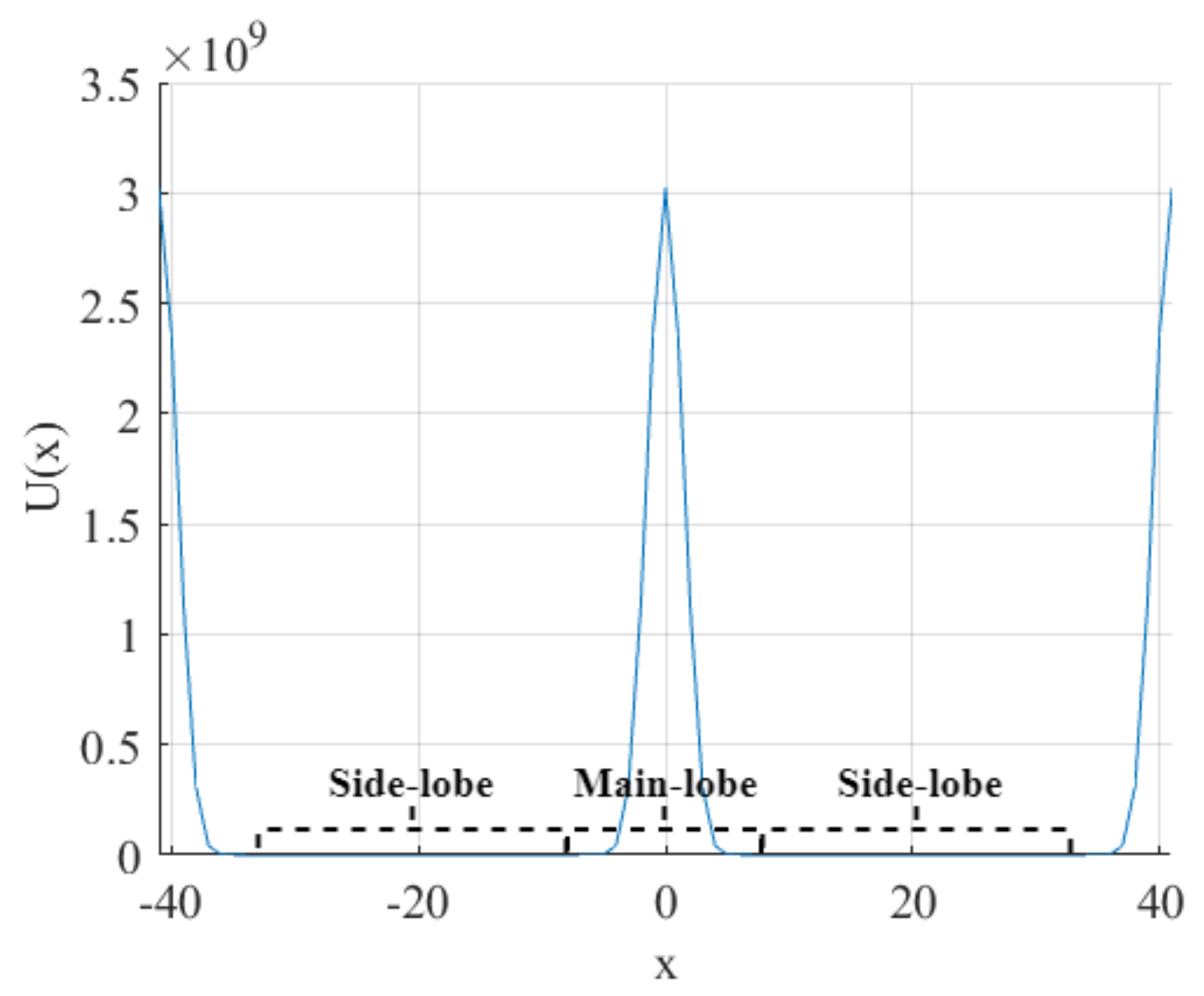
The parameter M is the function length and $\alpha$ is a parameter which controls the side-lobes level. An example of $U(x)$ is shown in Figure 2.

From Figure 2, it can be observed that $U(x)$ behaves like an inverted graph of the retinal vessels’ intensity profile. Moreover, $U(x)$ is a periodic function with $x\in \left[-\frac{M-1}{2},\frac{M-1}{2}\right]$, such that a truncation on that range of x will not cause any information loss. This makes an inverted $U(x)$ a more suitable model for the retinal vessels’ intensity profile. However, the sharp peak of $U(x)$ does not match the rounded vertices of the retinal vessels’ intensity profiles, particularly for those in Figure 1b,c. As a result, implementing the original Dolph-Chebyshev function as the basis function of a matched filter kernel may lead to an undesirable performance. Here, we propose the following modified Dolph-Chebyshev function:

$$W\left(x\right)=\left\{\begin{array}{cc}-\left|\frac{cos\left\{M{cos}^{-1}[\beta cos(\pi x\gamma )]\right\}}{cosh[M{cosh}^{-1}(\beta )]}\right|,\hfill & \left|A(x)\right|\le 1\hfill \\ -1,\hfill & \mathrm{otherwise}\hfill \end{array}\right.,$$

(4)

$$W^{\prime }(x)=W(x)-\overline{W(x)},$$

(5)

where

$$A(x)=\beta cos(\pi x\gamma ),$$

(6)

$$\beta =cosh[(1/M){cosh}^{-1}({10}^{\alpha })],$$

(7)

$$\alpha =log\left\{cosh\left[(M-1){cosh}^{-1}\left(sec\left(\frac{{\omega }_c\pi }{M}\right)\right)\right]\right\},$$

(8)

$$\gamma =1/(M+1),$$

(9)

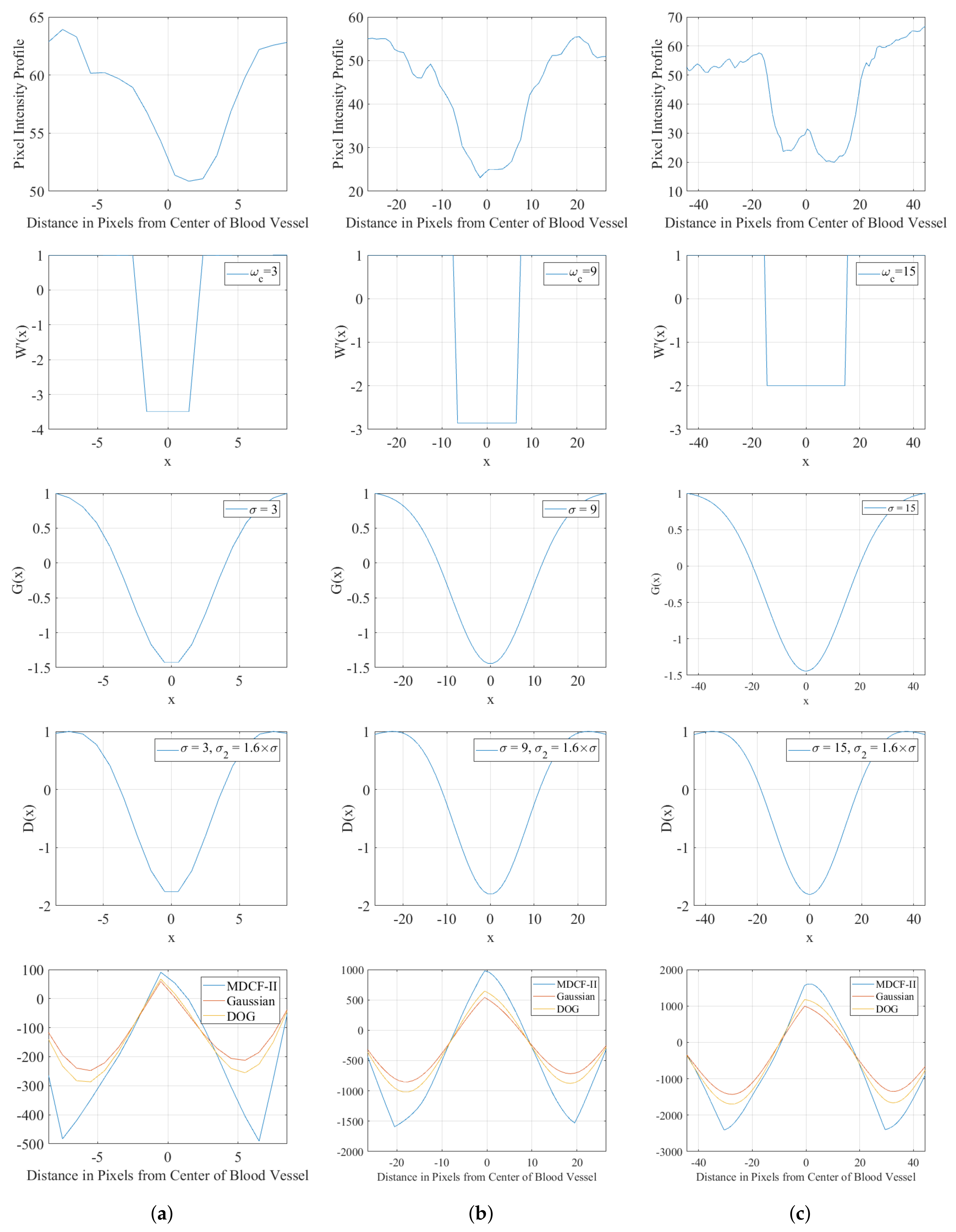
and $\overline{W\left(x\right)}$ is the mean of $W\left(x\right)$. For (4)–(9), x is defined on $x\in [-\frac{(M-1)}{2},\frac{(M-1)}{2}]$. $W(x)$ in (4) is proposed to have a pass band ($-{\omega }_c\le x\le {\omega }_c$) with a less-pointed vertice. Some graphs of $W(x)$ are shown in the second row of Figure 3. Then, by borrowing the term from the Chebyshev type II filter [19], we call the relations in (4)–(9) as the modified Dolph-Chebyshev type II function (MDCF-II) since the pass band does not have an equiripple property.

We have conducted an experimental setup to show that among other existing functions, such as the Gaussian and the Difference of Gaussian (DOG) as used in [2] and [20], respectively the MDCF-II provides a better model for the intensity profiles of retinal vessels’ cross-sections. In the experiment, the MDCF-II and other existing functions are convolved with the intensity profiles of the retinal vessels’ cross sections in Figure 1. We implement the functions with some values of scale (${\omega }_c$ in the MDCF-II and $\sigma$ in the Gaussian and the DOG), i.e., 3, 9 and 15 to approximate the thin, medium and thick vessels while the length $(M)$ of each function is set to be equal to six times of the scale’s value. The results for the thin, medium and thick vessels are shown in Figure 3a–c, respectively.

As depicted from the last row of Figure 3, the MDCF-II achieves highest convolutional responses and therefore would provide the best model for the thin, medium and thick vessels. Hence, we propose the MDCF-II with several values of ${\omega }_c$ to serve as a similar role like the Gaussian function in the conventional matched filter. To perform retinal vessel detection, the proposed matched filter is expanded in a 2-D form as follows:

$$W_i(x,y)=\left\{\begin{array}{cc}-\left|\frac{cos\left\{M{cos}^{-1}[\beta cos(\pi u\gamma )]\right\}}{cosh[M{cosh}^{-1}(\beta )]}\right|,\hfill & \left|A(x,y)\right|\le 1\hfill \\ -1,\hfill & \mathrm{otherwise}\hfill \end{array}\right.,$$

(10)

where

$$A(x,y)=\beta cos(\pi u\gamma ),$$

(11)

$$\left[\begin{array}{cc}u& v\end{array}\right]=\left[\begin{array}{cc}x& y\end{array}\right]\left[\begin{array}{cc}cos{\theta }_i& sin{\theta }_i\\ -sin{\theta }_i& cos{\theta }_i\end{array}\right].$$

(12)

$\left[\begin{array}{cc}x& y\end{array}\right]$ is the original coordinate system while $\left[\begin{array}{cc}u& v\end{array}\right]$ is the corresponding coordinate system rotated at an angle $\left({\theta }_i\right)$. The u and v points are defined on the neighborhood $N=\left\{(u,v)|-M/2<u<M/2,0<v\le T\right\}$. The kernel $W_i^{\prime }\left(x,y\right)$ is calculated at several angles to detect retinal vessels at all possible orientations. Finally, the mean of the template $W_i$ $(\overline{W_i})$ is subtracted from the template $W_i$ to have a zero-mean template $W_i^{\prime }$ as follows:

$$W_i^{\prime }(x,y)=W_i(x,y)-\overline{W_i},$$

(13)

where

$$\overline{W_i}=\sum _{\overline{p_i}ϵN}{W}_i(x,y)/S,$$

(14)

and S is the number of pixels in the neighborhood N.

3. Retinal Vessels Segmentation Using Proposed Matched Filter

3.1. Pre-Processing and Post-Processing Phases

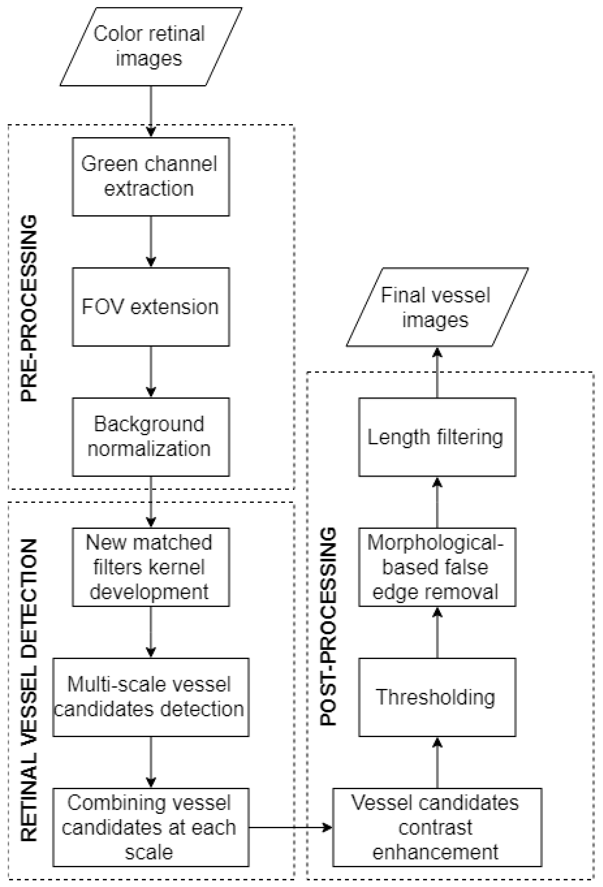
Our algorithm for retinal vessels segmentation includes the main phase which is the retinal vessel detection using the proposed matched filter as well as a pre-processing and a post-processing phases. A schematic diagram for the proposed algorithm is shown in Figure 4. The pre-processing phase consists of green channel $(I_{green})$ extraction, field of view (FOV) extension and background normalization. $I_{green}$ is chosen since it presents the best vessels to background contrast among other channels. Then, the FOV is extended using the method in [9] to remove a sharp change between the FOV and the region beyond the FOV.

The background normalization step is beneficial in removing exudates which may appear in the fundus image as well as in improving the vessels to background contrast. The exudates are removed using the in-painting technique in [5] while the vessels contrast is enhanced using contrast-limited histogram equalization (CLAHE). In using the in-painting method, we need to define the kernel size of the median filter for the DRIVE database since those were not specified by [5]. The size is determined based on the one used in the STARE database. In addition, we propose an adaptive thresholding method to further improve the performance of exudates detection in [5] as follows:

$$T=\left\{\begin{array}{cc}{T}_{OTSU},\hfill & T_{OTSU}\ge \overline{I}\hfill \\ 165,\hfill & otherwise\hfill \end{array}\right..$$

(15)

$T_{OTSU}$ is a threshold value for the image I obtained using the Otsu’s method [21] while $\overline{I}$ is the average intensity of I. We have conducted an experiment and found that the constant threshold value of 165 as suggested in [5] is optimum for the situation where $T_{OTSU}\ge \overline{I}$.

The post-processing phase is required to obtain final images of segmented blood vessels. This phase comprises of vessels candidates’ contrast enhancement, thresholding, vessel’s edge refinement and length filtering. The contrast of the retinal vessel candidates is improved using a linear contrast stretching technique. The thresholding aims to convert the detected retinal vessels into a binary image using a threshold value $T_B$. In this paper, $T_B$ for each image is calculated using second-order entropy-based thresholding [22]. The thresholding method has two advantages. First, it has an ability to takes into account the spatial distribution of gray-levels retinal vessels, which are not independent of each other. Moreover, the algorithm is able to preserve the spatial structures in the binary vessel image [22].

As a result of thresholding, there are some edges not belonging to vessels but emerge in the surrounding since we apply a global threshold value to binarize all retinal vessels. To address this problem, we follow a morphological-based elimination strategy used by [23]. In the last stage, a length filter with a threshold value $T_L$ is used to remove the remaining undesirable objects. $T_L$ for the DRIVE database is set to be equal to 250 [24] while the values for the STARE and HRF databases are determined based on the DRIVE database ($T_L=$ 250). The procedure to set $T_L$ for the STARE and HRF databases will be discussed in Section 3.3.

3.2. Retinal Vessels Detection Phase

The retinal vessels are detected by convolving the pre-processed image with the matched filter window at a particular scale ${\omega }_{c,j}$ and orientation ${\theta }_i$ to get a vessel image $R_{i,j}$ as follows:

$$R_{i,j}(x,y)=I(x,y)*W_{i,j}^{\prime }(x,y).$$

(16)

We utilize 12 $\theta$ values ($\theta =\left\{0^{\circ },{15}^{\circ },{30}^{\circ },\cdots ,{165}^{\circ }\right\}$) in calculating $W_i^{\prime }\left(x,y\right)$. Subsequently, the retinal vessel image at certain scale $R_{max,j}$ is obtained by taking the maximum response of $R_{1,j}$ to $R_{12,j}$:

$$R_{max,j}=max(R_{1,j},R_{2,j},...,R_{12,j}).$$

(17)

Having obtained $R_{max,j}$ at all scales $(j=1,2,\cdots ,J)$, we use a new method which is a modification from that in [4] to combine $R_{max,1}$ to $R_{max,J}$ as follows:

$$R_{combined}=\sum _{j=1}^J\left(w_j{R}_{std,j}+\frac{1}{J+1}{I}_{std}\right),$$

(18)

where

$$w_j=\frac{exp\left(-\tau \left({\omega }_{c,j}-{\tilde{\omega }}_{c,j}\right)\right)}{1-exp\left(-\tau \left({\omega }_{c,j}-{\tilde{\omega }}_{c,j}\right)\right)},$$

(19)

$$R_{std,j}=\frac{R_{max,j}-\overline{R_{max,j}}}{{\sigma }_{R_{max,j}}}.$$

(20)

$R_{combined}$, $R_{std,j}$, $\overline{R_{max,j}}$ and ${\sigma }_{R_{max,j}}$ are the combined matched filter’s responses, the standardized matched filter’s response, the average intensity of $R_{max,j}$ and the standard deviation of $R_{max,j}$, respectively. The standardization aims to enhance the contrast of vessels to background but without changing the distribution of the pixels’ intensity values [4].

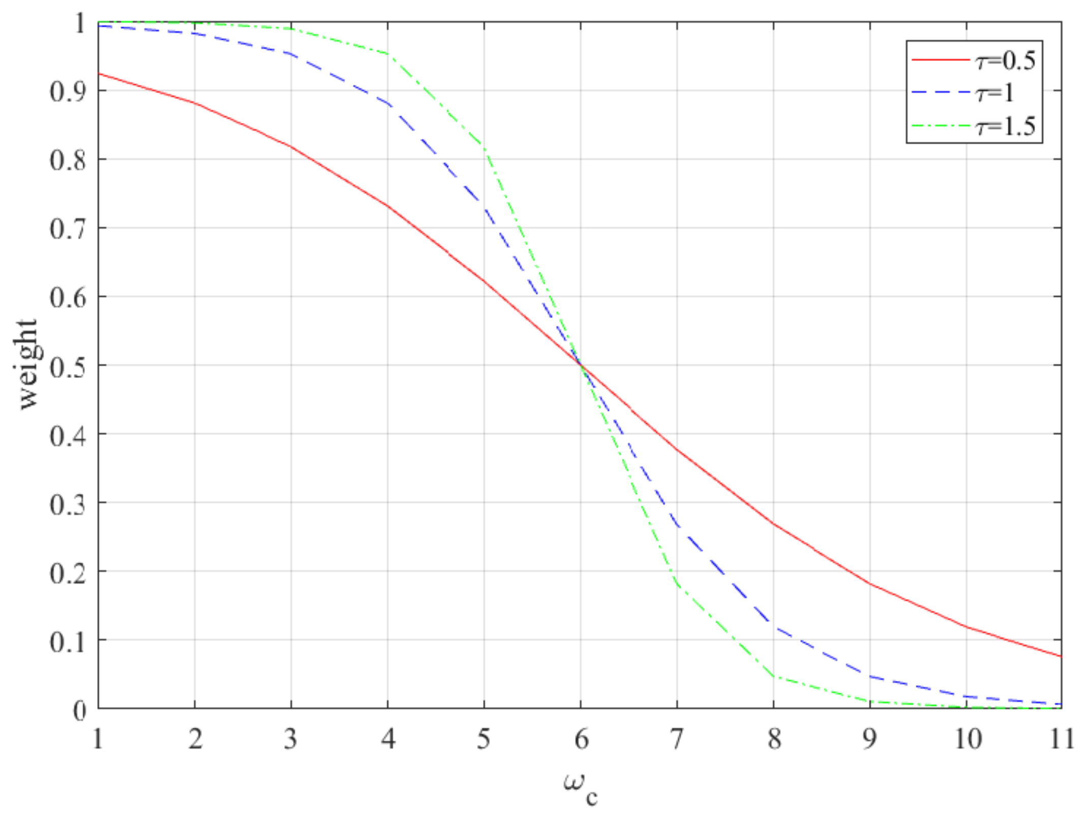
It is interesting to note that we have a parameter $\tau$ which controls the weight $\left(w_j\right)$ for each $R_{std,j}$. This parameter has a value of $\tau \ge 0$. Figure 5 depicts an example of $w_j$ with several values of $\tau$, in which a large $\tau$’s value corresponds to a large weight for $R_{std,j}$ with a small ${\omega }_{c,j}$ value. On the contrary, a large weight for $R_{max,j}$ with a large value of ${\omega }_{c,j}$ can be obtained using a small value of $\tau$. Hence, a suitable value of $\tau$ for the images from a particular database is required, such that a simple global thresholding technique can be applied to segment retinal vessels with all possible widths simultaneously.

3.3. Parameter Setting

In this section, we present the procedures to set the parameters’ values of the median filter, matched filter and length filter. The unassigned parameters’ values on a particular database are calculated based on the values of the corresponding parameters specified earlier on another database. For instance, the kernel size of the median filter on the STARE database which is taken from the work of [5] is used to determine the corresponding parameter’s value on the DRIVE database. On the contrary, $T_L=250$ for the length filter on the DRIVE database which is adapted from [24] is utilized to specify the $T_L$’s values on the STARE and HRF databases. Those parameters’ values can be calculated as follows:

$$P_A=P_B\times s_{A,B},$$

(21)

where

$$s_{A,B}=0.5\times (\frac{X_A}{X_B}+\frac{Y_A}{Y_B}).$$

(22)

The variables $X_A$ and $Y_A$ are the length and width of an image from the database A while $s_{A,B}$ is the size ratio of the image from databases A and B. The variable $P_A$ is the parameter’s value for particular database A. If $P_A$ is $T_{L,A}$, A refers to the STARE database or the HRF database, while B is for the DRIVE database. On the other hand, $P_A$ is the kernel size of the median filter and A and B represent the DRIVE and STARE databases as we want to define the kernel size of the median filter on the DRIVE database.

The parameters’ values of the proposed matched filter are determined by adopting those in the conventional matched filter [2] with several modifications. In accordance with the work in [2], we start defining the values on the DRIVE database while the values for the STARE and HRF databases can be calculated based on those for the DRIVE database. In MDCF-II, ${\omega }_c$ is the most important parameter since it governs the main lobe width and at the same time, it is related to retinal vessels’ widths. To set the ${\omega }_c$ value, we follow the similar procedure as in [2], in which the average width of retinal vessels was used to set the main lobe width of the Gaussian function $(\sigma )$.

Besides ${\omega }_c$, we have to define the values of m, t, M and T. m and t are the length and width of the proposed matched filter kernel. A series of experiments have been conducted to find those values using ${\omega }_c=2$ (since $\sigma =2$ in [2]). From the experiment, we found that $m=17$, $t=16$, $M=12$ and $T=8$ provided better performance than $m=16$, $t=15$, $M=13$ and $T=9$ as used in [2]. Based on the assigned values of ${\omega }_c$, m, t, M and T, we are able to define the ratios of M, T and t to ${\omega }_c$ as $r_M$, $r_T$ and $r_t$, which are equal to 6, 4 and 8, respectively. Subsequently, we define a relation of m and t as follows:

$$m=t+1.$$

(23)

We utilize the procedure in setting the ${\omega }_c$’s values, the ratios and the expression in (23) to set the parameters’ values of our matched filter bank on the DRIVE, STARE and HRF databases.

4. Experimental Results and Discussions

The proposed algorithm is simulated using 40 low-resolution fundus images from the DRIVE and STARE databases and 45 high-resolution fundus images from the HRF database on a computer with i7 core processor and 8GB RAM. Each of the DRIVE and STARE databases consists of 20 images with sizes of 565 × 584 and 700 × 605 pixels, respectively. On the other hand, the HRF database comprises the healthy, diabetic retinopathy and glaucomatous sets. Each set includes 15 high-resolution fundus images with a size of 3504 × 2336 pixels. The three databases provide the ground truths as the results of manual vessels segmentations.

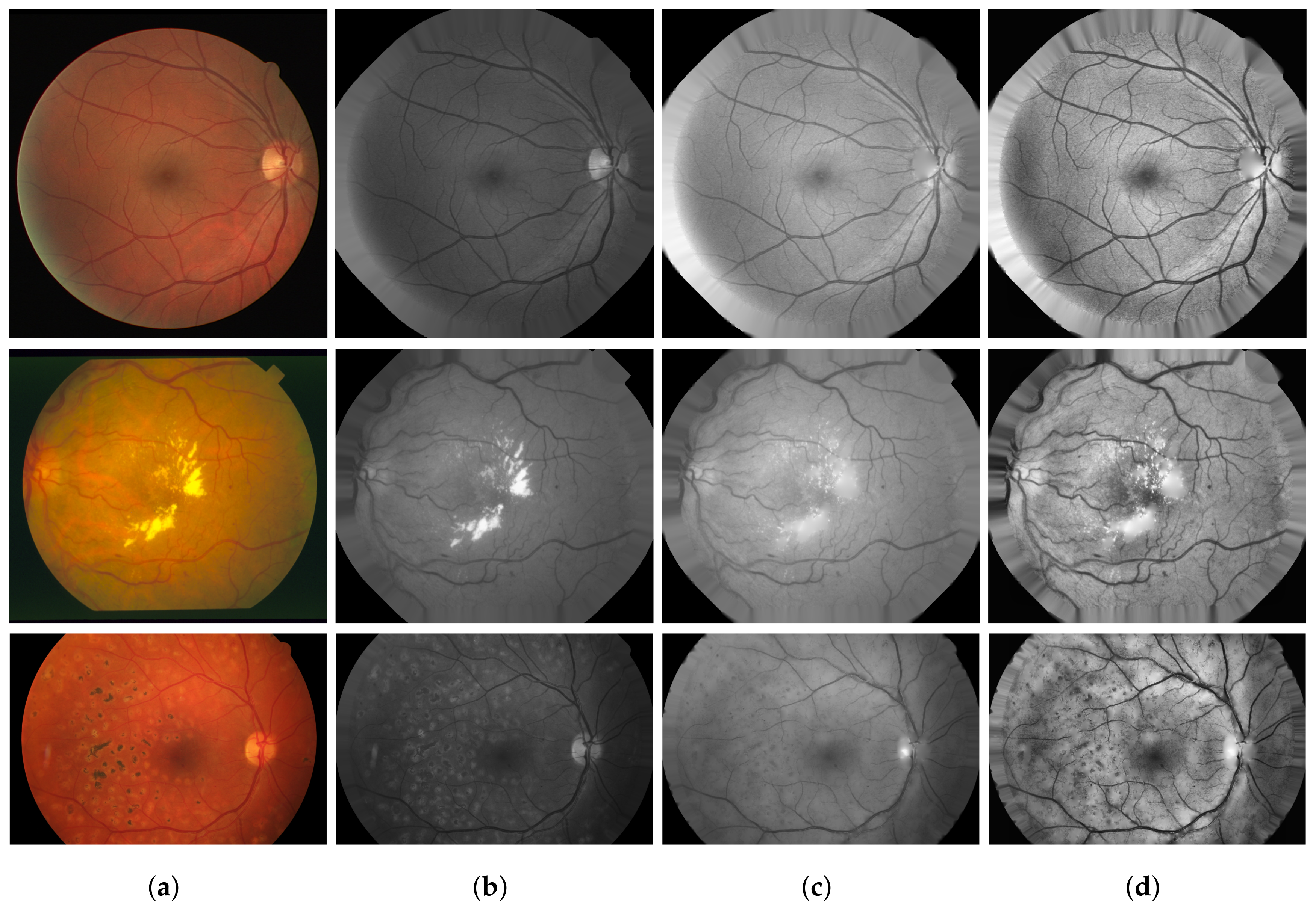
Figure 6a–d show the original color fundus images, the results of the FOV extension, the in-painted images and the results of CLAHE, respectively. The top, middle and bottom rows of Figure 6 are for the images from the DRIVE, STARE and HRF databases, respectively. As can be observed in Figure 6d, the pre-processing phase effectively provides high-contrast and exudate-free images, such that the subsequent phases can be performed optimally.

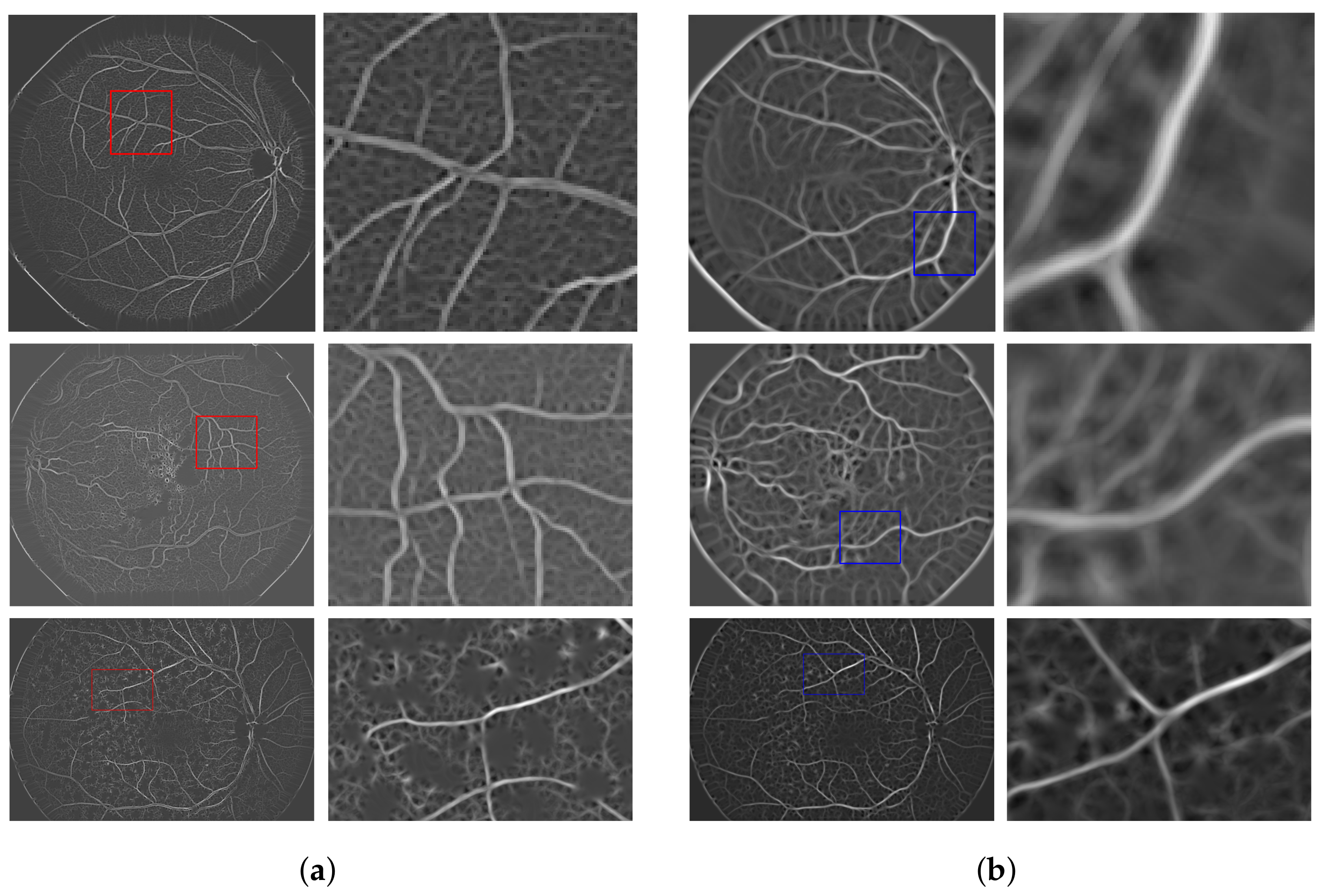
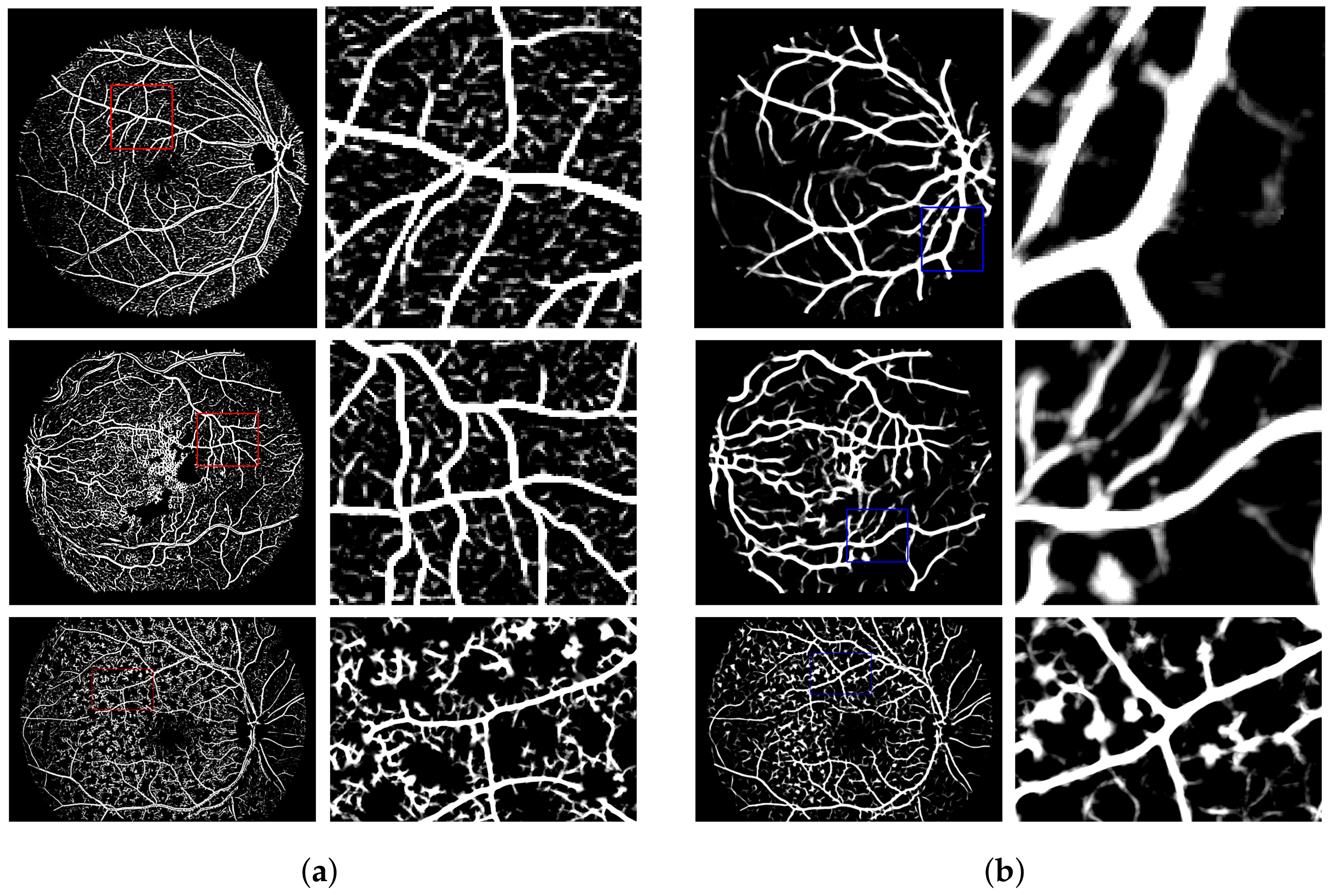
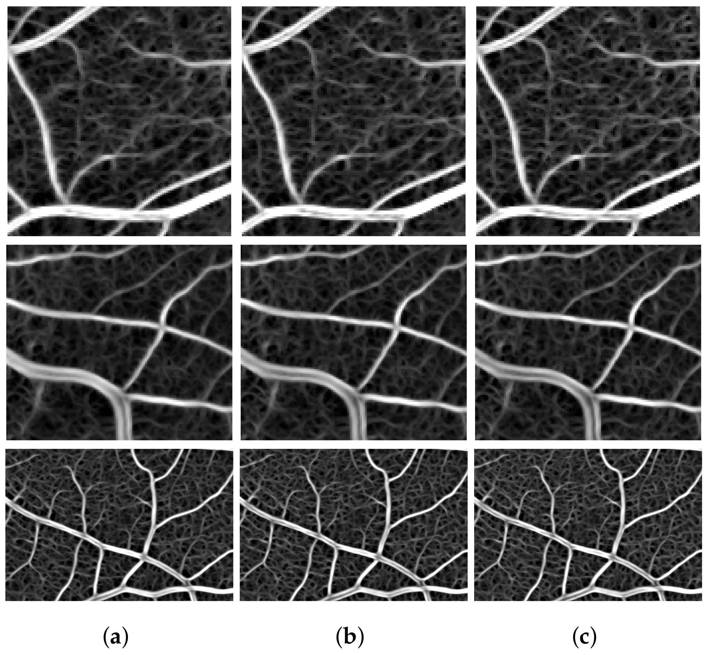
After obtaining the pre-processed image, the retinal vessels detection phase is performed. $R_{i,j}$ and $R_{max,j}$ are obtained using (16) and (17), respectively. Subsequently, $R_{std,j}$ is calculated using (20). Figure 7a,b show some examples of $R_{max,j}$ with small and large values of ${\omega }_c$, respectively. The left and right columns of both Figure 7a,b indicate full images and excerpts of $R_{max,j}$. The first, second and third rows of Figure 7 describe the images from the DRIVE, STARE and HRF databases. Small values of ${\omega }_c$ for the three databases are equal to 1, 1 and 5, while 5, 5 and 15 are large values of ${\omega }_c$ for the three databases, respectively. Furthermore, Figure 8 depicts some examples of $R_{std,j}$ with similar configuration to that of Figure 7.

Figure 7 indicates that our matched filter bank effectively detects retinal vessels at all possible orientations and different widths. For instance, the thin vessels are effectively detected using a small ${\omega }_c$’s value (see Figure 7a). It is observed that applying the proposed matched filter at different scales is necessary to obtain a complete vessel response $R_{combined}$. To calculate $R_{combined}$, we use $R_{std,j}$ as it provides a better contrast of the vessel to background than that of $R_{max,j}$ (see Figure 8). In calculating $R_{combined}$, we use ${\omega }_c$’s values in the range of ${\mathsf{\Omega }}_c=\{{\omega }_c|{\omega }_{c,min}\le {\omega }_c\le {\omega }_{c,max}\}$, where ${\omega }_{c,min}$ and ${\omega }_{c,max}$ are the minimum and maximum radii of retinal vessels on the image from a certain database. For the DRIVE and STARE databases, ${\omega }_{c,min}$ and ${\omega }_{c,max}$ are equal to 1 and 5 [6,17] while ${\omega }_{c,min}$ and ${\omega }_{c,max}$ for the HRF database are equal to 3 and 15 [3,5] respectively.

Aside from ${\omega }_c$’s values, we have to define the values of $\tau$. Some examples of $R_{combined}$ with $\tau =$ 0.5, 1 and 1.5 for the image from all databases are provided in Figure 9a–c, respectively. The first, second and third rows of Figure 9 indicate the images from the DRIVE, STARE and HRF databases. As can be observed in Figure 9, the thin vessels can be effectively segmented using a high value of $\tau$, but we may not be able to preserve the complete structure of the thick vessels, particularly for those with the central reflex as shown in Figure 9c.

It is interesting to note that segmenting all types of vasculatures at the same time is much desirable. For this purpose, the $\tau$ value for each database is determined based on the distribution of vessels widths of the image from each database. For instance, if the average radii of the blood vessels $({\overline{\omega }}_c)$ on a particular database is larger than $\frac{{\omega }_{c,min}+{\omega }_{c,max}}{2}$, then the majority of vessels pixels are on the medium and thick blood vessels. On the other hand, ${\overline{\omega }}_c\le \frac{{\omega }_{c,min}+{\omega }_{c,max}}{2}$ indicates that the corresponding database contains a larger amount of thin and medium blood vessels pixels than those of thick vasculatures. The values of ${\omega }_{c,min}$, ${\overline{\omega }}_c$ and ${\omega }_{c,max}$ for images from the DRIVE and STARE databases are 1, 3 and 5 while 3, 12.5 and 15 are the corresponding values for images from the HRF database. These indicate that the majority of the vessels’ pixels in the DRIVE and STARE databases belong to thin and medium blood vessels while the HRF database takes the opposite.

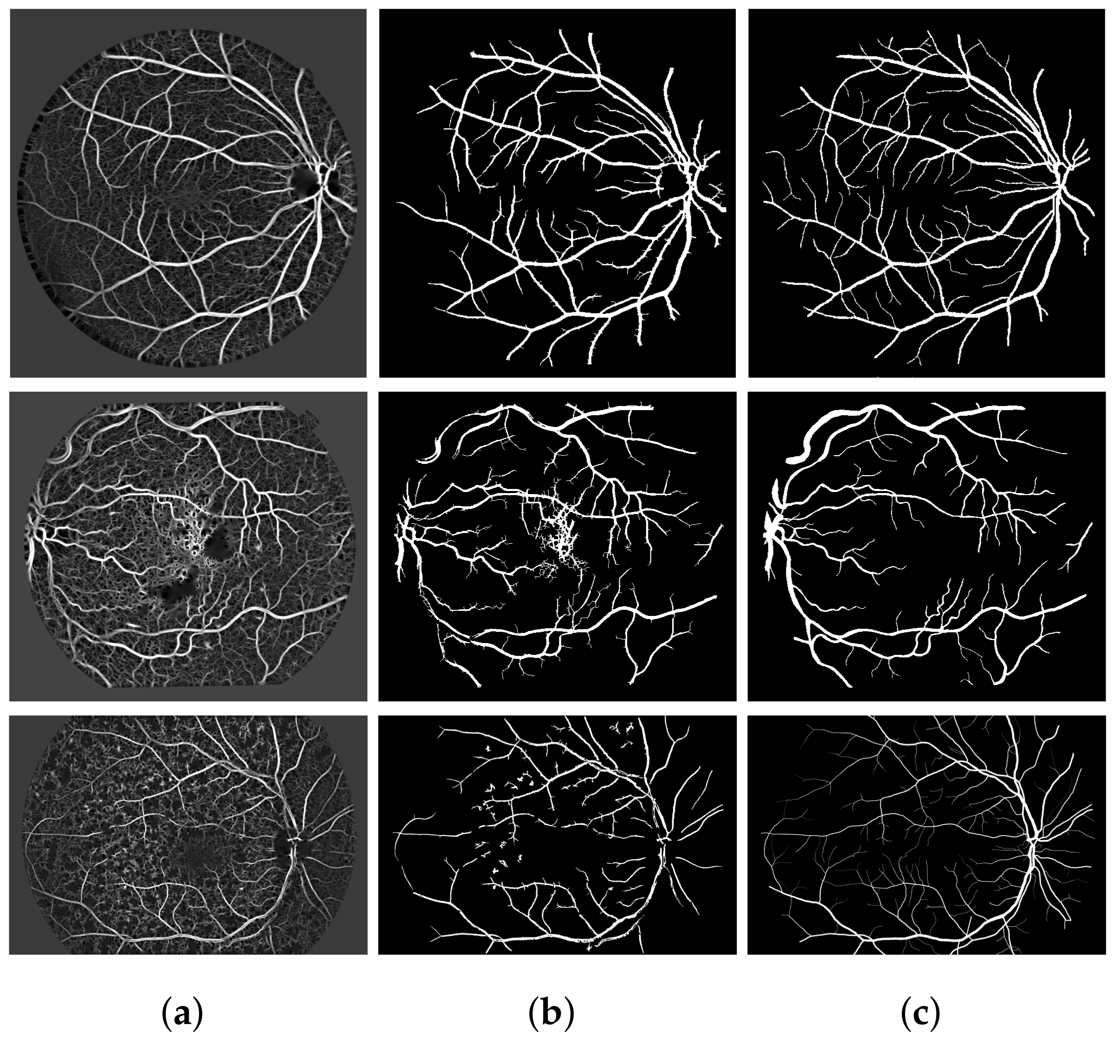
The final vessel image is obtained by applying the steps in the post-processing phase to $R_{combined}$. Some examples of $R_{combined}$, the post-processed image and the corresponding ground truths are depicted in Figure 10a–c, respectively. The first, second and third rows of Figure 10 describe the images from the DRIVE, STARE and HRF databases. As shown in Figure 9a, the combination method with chosen values of $\tau$ effectively incorporates the matched filter’s responses, such that $R_{combined}$ contains the detected blood vessels with most of the widths. Finally, the steps in the post-processing phase are able to provide the final vessel images which highly match the corresponding ground truths as shown in Figure 10b,c.

5. Discussion

5.1. Performance Measure of the Proposed Algorithm

The performance of our algorithm is evaluated in terms of sensitivity $(Se)$, specificity $(Sp)$, positive predictive value $(Ppv)$, F1-Score $(F1)$, G-mean $(G)$ and Matthews correlation coefficient $(MCC)$ for the region inside FOV. Although accuracy $(Acc)$ is widely used to quantify the performance of existing methods, $(Acc)$ alone, however, is not sufficient for quantifying vessels segmentation efficacy since it too much reflects $Sp$ and moreover, majority of retinal pixels are not vessels type. Hence, we use $F1$, G and $MCC$ since they are more suitable for imbalanced class ratios [13]. Details of the measures can be found in [13] and can be expressed as follows:

$$Se=\frac{TP}{TP+FN},$$

(24)

$$Sp=\frac{TN}{TN+FP},$$

(25)

$$Ppv=\frac{TP}{TP+FP},$$

(26)

$$F1=\frac{2Ppv\times Se}{Ppv+Se},$$

(27)

$$G=\sqrt{Se\times Sp},$$

(28)

$$MCC=\frac{TP/N-S\times P}{\sqrt{P\times S\times \left(1-S\right)\times \left(1-P\right)}},$$

(29)

where N is the number of pixels within an image, $S=(TP+FP)/N$ and $P=(TN+FP)/N$.

The performance of our algorithm and other methods published in the past five years on the low and high-resolution fundus images are presented in

Table 1. Performance of Vessel Segmentation Methods on Low-Resolution Images from the DRIVE and STARE databases.

Database:	DRIVE (Test Set)						STARE
Method	Se	Sp	Ppv	F1	G	MCC	Se	Sp	Ppv	F1	G	MCC
Unsupervised
Nguyen et al. [4]	0.742	0.970	0.783	0.762	0.848	0.728	0.785	0.950	0.648	0.704	0.862	0.674
Odstrcilik et al. [3]	0.706	0.969	−	−	0.827	−	0.785	0.951	−	−	0.864	−
Roychowdurry et al. [7]	0.739	0.978	−	−	0.850	−	0.732	0.984	−	−	0.849	−
Zhao et al. [8]	0.742	0.982	−	−	0.854	−	0.780	0.978	−	−	0.873	−
Annunziata et al. [5]	−	−	−	−	−	−	0.713	0.984	0.833	0.768	0.838	−
Nergiz and Akin [25]	0.812	0.934	−	−	−	−	0.813	0.944	−	−	−	−
Proposed Method	0.748	0.978	0.833	0.786	0.856	0.758	0.793	0.973	0.772	0.780	0.877	0.756
Supervised
Dai et al. [11]	0.736	0.972	−	−	0.846	−	0.777	0.955	−	−	0.861	−
Roychowdurry et al. [10]	0.725	0.983 ${}^{†}$	−	−	0.844	−	0.772	0.973	−	−	0.867	−
Li et al. [12]	0.757	0.982	−	−	0.862	−	0.773	0.984	−	−	0.872	−
Liskowski et al. [14]	0.775	0.979	−	−	0.871	−	0.777	0.985 ${}^{†}$	−	−	0.878	−
Orlando et al. [13]	0.790	0.968	0.785	0.786	0.874	0.756	0.768	0.974	0.774	0.764	0.863	0.742
Fu et al. [15]	0.760	−	−	−	−	−	0.741	−	−	−	−	−
Zhou et al. [16]	0.808 ${}^{†}$	0.967	0.786 ${}^{†}$	0.794 ${}^{†}$	0.883 ${}^{†}$	0.766 ${}^{†}$	0.806 ${}^{†}$	0.976	0.811 ${}^{†}$	0.802 ${}^{†}$	0.886 ${}^{†}$	0.783 ${}^{†}$

† The best value for supervised methods.

and

Table 2. Performance of Vessel Segmentation Methods on High-Resolution Images from the HRF database.

Method	Se	Sp	Ppv	F1	G	MCC
Odstrcilik et al. [3]	0.779	0.965	0.695	0.732	0.867	0.707
Annunziata et al. [5]	0.713	0.984	0.809	0.758	0.838	−
Orlando et al. [13]	0.787	0.958	0.663	0.716	0.869	0.690
Zhou et al. [16]	0.802	0.970	0.733	0.763	0.881	0.740
Proposed Method	0.804	0.971	0.733	0.764	0.883	0.741

, respectively. In Table 1, the highest value on each quantitative measure for the unsupervised methods is listed in bold while that for the supervised methods is marked with a dagger $(†)$. It is observed from Table 1 and Table 2 that our algorithm outperforms all other unsupervised methods in terms of $F1$, G and $MCC$. In addition, we are able to achieve higher $Se$ scores than most of unsupervised methods, except for the method in [25]. However, the method in [25] is prone to a huge number of false positives (on exudates and optical disc boundaries), which is indicated by its lowest $Sp$ scores compared to other presented methods. This is undesirable, particularly when it is applied on fundus images with many pathological signs, for instances exudates.

It is interesting to note that our achieved $Se$ and G scores on low-resolution images are better than those of some supervised methods, i.e., the methods in [10,11,15]. The proposed algorithm is also more robust than those supervised methods as it performs better on the STARE database, which consists of images with many pathological indications. Although on low-resolution images the methods in [14,16] achieve relatively better performance than ours, the efficacy of the method in [14] has not been tested on high-resolution images while the convolutional neural network (CNN) used in [16] is highly complex, such that the high-resolution images from the HRF database are required to be downsampled to reduce the complexity (See [16] for details). As a result, on the high-resolution fundus images, this method is not able to achieve similar superior performance as achieved on the low-resolution fundus images. Since our algorithm is able to achieve superior performance on the high-resolution fundus images and does not require high-resolution fundus images to be downsampled, it may be suitable for large-scale applications such as automatic detection tool for retinal diseases, particularly where high-resolution fundus images are utilized.

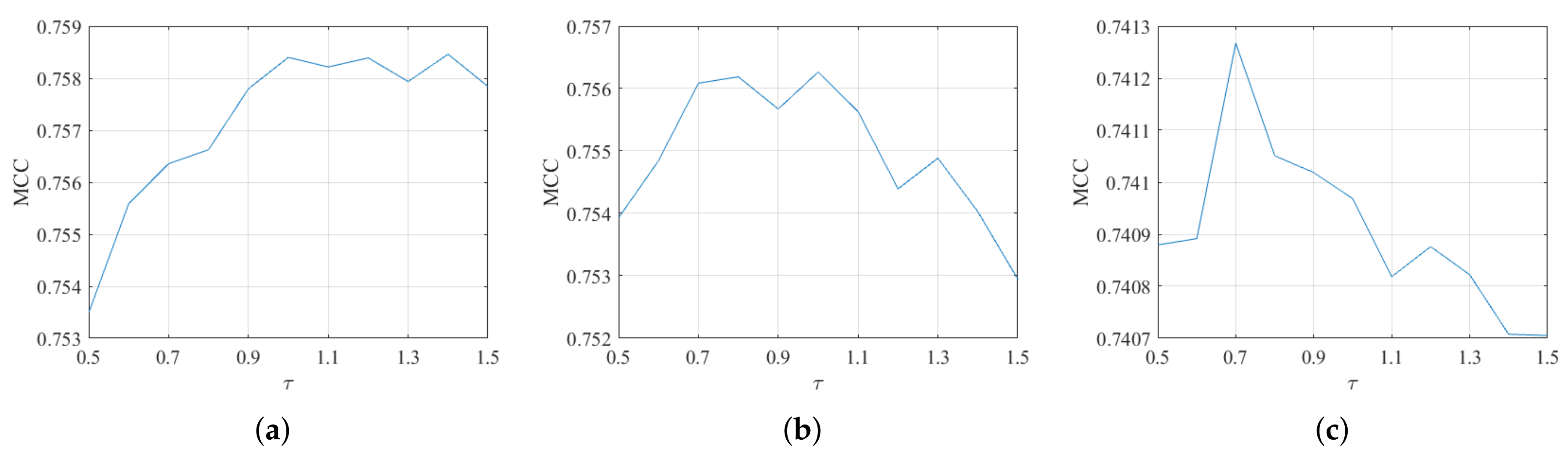
5.2. The Performance of the Proposed Algorithm with Different $\tau$ Values

As mentioned earlier, the value of $\tau$ plays an important role in calculating weights for matched filter responses at different scales. In this section, we present sensitivity analysis of the $\tau$ value to the segmentation efficacy. We conduct an experimental setup for each database using several values of $\tau$ ($\tau =\{0.5,0.6,\cdots ,1.5\}$). The effects of $\tau$ values for each database to the segmentation efficacy are presented in $MCC$ versus $\tau$ graphs (See Figure 11).

6. Conclusions

A new unsupervised algorithm for retinal vessels segmentation is presented in this paper. The algorithm uses a novel matched filter bank with MDCF-II and a new method to combine the matched filter’s responses. The performance of the proposed algorithm has been evaluated using the fundus images from the DRIVE and STARE databases as well as the high-resolution fundus images from the HRF database. Among other unsupervised methods, the proposed algorithm achieves the best performance both for the low and high-resolution fundus images. In addition, the proposed algorithm is able to outperform the supervised methods, particularly for the high-resolution fundus images. This is beneficial since high-resolution fundus images are more common and will be more useful.

References

- Salazar-Gonzalez, A.; Kaba, D.; Li, Y.; Liu, X. Segmentation of Blood Vessels and Optic Disc in Retinal Images. IEEE J. Biomed. Health Inform. 2014, 2194, 1874–1886. [Google Scholar] [CrossRef] [PubMed]
- Chaudhuri, S.; Chatterjee, S.; Katz, N.; Nelson, M.; Goldbaum, M. Detection of blood vessels in retinal images using two-dimensional matched filters. IEEE Trans. Med. Imaging 1989, 8, 263–269. [Google Scholar] [CrossRef] [PubMed]
- Odstrcilik, J.; Kolar, R.; Kubena, T.; Cernosek, P.; Budai, A.; Hornegger, J.; Gazarek, J.; Svoboda, O.; Jan, J.; Angelopoulou, E. Retinal vessel segmentation by improved matched filtering: Evaluation on a new high-resolution fundus image database. IET Image Process. 2013, 7, 373–383. [Google Scholar] [CrossRef]
- Nguyen, U.T.V.; Bhuiyan, A.; Park, L.A.F.; Ramamohanarao, K. An effective retinal blood vessel segmentation method using multi-scale line detection. Pattern Recognit. 2013, 46, 703–715. [Google Scholar] [CrossRef]
- Annunziata, R.; Garzelli, A.; Ballerini, L.; Mecocci, A.; Trucco, E. Leveraging Multiscale Hessian-Based Enhancement with a Novel Exudate Inpainting Technique for Retinal Vessel Segmentation. IEEE J. Biomed. Health Inform. 2016, 20, 1129–1138. [Google Scholar] [CrossRef] [PubMed]
- Staal, J.J.; Abramoff, M.D.; Niemeijer, M.; Viergever, M.A.; Van Ginneken, B. Ridge based vessel segmentation in color images of the retina. IEEE Trans. Med. Imaging 2005, 23, 501–509. [Google Scholar] [CrossRef] [PubMed]
- Roychowdhury, S.; Koozekanani, D.D.; Parhi, K.K. Iterative Vessel Segmentation of Fundus Images. IEEE Trans. Biomed. Eng. 2015, 62, 1738–1749. [Google Scholar] [CrossRef] [PubMed]
- Zhao, Y.; Rada, L.; Chen, K.; Harding, S.P.; Zheng, Y. Automated Vessel Segmentation Using Infinite Perimeter Active Contour Model with Hybrid Region Information with Application to Retinal Images. IEEE Trans. Med. Imaging 2015, 34, 1797–1807. [Google Scholar] [CrossRef] [PubMed]
- Soares, J.V.B.; Leandro, J.J.G.; Cesar, R.M.J.; Jelinek, H.F.; Cree, M.J. Retinal Vessel Segmentation Using the 2-D Gabor Wavelet and Supervised Classification. IEEE Trans. Med. Imaging 2006, 25, 1214–1222. [Google Scholar] [CrossRef] [PubMed] [Green Version]
- Roychowdhury, S.; Koozekanani, D.D.; Parhi, K.K. Blood vessel segmentation of fundus images by major vessel extraction and subimage classification. IEEE J. Biomed. Health Inform. 2015, 19, 1118–1128. [Google Scholar] [CrossRef] [PubMed]
- Dai, P.; Luo, H.; Sheng, H.; Zhao, Y.; Li, L.; Wu, J.; Zhao, Y.; Suzuki, K. A new approach to segment both main and peripheral retinal vessels based on gray-voting and Gaussian mixture model. PLoS ONE 2015, 10. [Google Scholar] [CrossRef] [PubMed]
- Li, Q.; Feng, B.; Xie, L.; Liang, P.; Zhang, H.; Wang, T. A cross-modality learning approach for vessel segmentation in retinal images. IEEE Trans. Med. Imaging 2016, 35, 109–118. [Google Scholar] [CrossRef] [PubMed]
- Orlando, J.I.; Prokofyeva, E.; Blaschko, M.B. A Discriminatively Trained Fully Connected Conditional Random Field Model for Blood Vessel Segmentation in Fundus Images. IEEE Trans. Biomed. Eng. 2017, 64, 16–27. [Google Scholar] [CrossRef] [PubMed] [Green Version]
- Liskowski, P.; Krawiec, K. Segmenting Retinal Blood Vessels With Deep Neural Networks. IEEE Trans. Med. Imaging 2016, 35, 2369–2380. [Google Scholar] [CrossRef] [PubMed]
- Fu, H.; Xu, Y.; Lin, S.; Kee, D.W.; Liu, J. DeepVessel: Retinal Vessel Segmentation via Deep Learning and Conditional Random Field. In Medical Image Computing and Computer-Assisted Intervention—MICCAI 2016; Ourselin, S., Joskowicz, L., Sabuncu, M.R., Unal, G., Wells, W., Eds.; Springer: Cham, Switzerland, 2016; pp. 132–139. [Google Scholar]
- Zhou, L.; Yu, Q.; Xu, X.; Gu, Y.; Yang, J. Improving dense conditional random field for retinal vessel segmentation by discriminative feature learning and thin-vessel enhancement. Comput. Methods Programs Biomed. 2017, 148, 13–25. [Google Scholar] [CrossRef] [PubMed]
- Hoover, A.; Kouznetsova, V.; Goldbaum, M. Locating blood vessels in retinal images by piecewise threshold probing of a matched filter response. IEEE Trans. Med. Imaging 2000, 19, 203–210. [Google Scholar] [CrossRef] [PubMed] [Green Version]
- Dolph, C. A Current Distribution for Broadside Arrays Which Optimizes the Relationship between Beam Width and Side-Lobe Level. Proc. IRE 1946, 34, 335–348. [Google Scholar] [CrossRef]
- Williams, A.B.; Taylor, F.J. Electronic Filter Design Handbook, 4th ed.; The McGraw-Hill Companies, Inc.: Singapore, 2006. [Google Scholar]
- Xiao, Z.; Wang, M.; Zhang, F.; Geng, L.; Wu, J.; Su, L.; Tong, J. Retinal vessel segmentation based on adaptive difference of Gauss filter. In Proceedings of the 2016 IEEE International Conference on Digital Signal Processing (DSP), Beijing, China, 16–18 October 2016; pp. 15–19. [Google Scholar] [CrossRef]
- Otsu, N. A Threshold Selection Method from Gray-Level Histograms. IEEE Trans. Syst. Man Cybern. 1979, 9, 62–66. [Google Scholar] [CrossRef]
- Chanwimaluang, T.; Fan, G.F.G. An efficient blood vessel detection algorithm for retinal images using local entropy thresholding. In Proceedings of the 2003 International Symposium on Circuits and Systems, Bangkok, Thailan, 25–28 May 2003; Volume 5, pp. 21–24. [Google Scholar] [CrossRef]
- Miri, M.S.; Mahloojifar, A. Retinal image analysis using curvelet transform and multistructure elements morphology by reconstruction. IEEE Trans. Biomed. Eng. 2011, 58, 1183–1192. [Google Scholar] [CrossRef] [PubMed]
- Ardizzone, E.; Pirrone, R.; Gambino, O.; Radosta, S. Blood Vessels and Feature Points Detection on Retinal Images. In Proceedings of the 30th Annual International EEE Engineering in Medicine and Biology Society Conference, Vancouver, BC, Canada, 20–25 August 2008; pp. 2246–2249. [Google Scholar] [CrossRef]
- Nergiz, M.; Akin, M. Retinal vessel segmentation via structure tensor coloring and anisotropy enhancement. Symmetry 2017, 9, 276. [Google Scholar] [CrossRef]
Figure 1.
Some examples of retinal vessels’ cross sections (top row) and their corresponding intensity profiles (bottom row) with (a) thin; (b) medium; and (c) thick widths.
Figure 2.
An example of the Dolph-Chebyshev function on with M = 42 and = 7.
Figure 3.
Convolution performance (fifth row) of intensity profiles of (a) thin; (b) medium; and (c) thick retinal vessels’ cross sections (first row) with MDCF-IIs (second row), Gaussian functions (third row) and DOG functions (fourth row).
Figure 4.
A schematic diagram for the proposed algorithm.
Figure 5.
An example of with 0.5, 1 and 1.5.
Figure 6.
(a) Original color fundus images; (b) green channel images; (c) in-painted images; and (d) CLAHE results. Top, middle and bottom rows: images from the DRIVE, STARE and HRF databases.
Figure 7.
Some examples of for (a) small and (b) large ’s values. Top, middle and bottom rows indicates the images from the DRIVE, STARE and HRF databases, respectively.
Figure 8.
Figure 9.
Some examples of with (a) 0.5, (b) 1 and (c) 1.5 for the image from the DRIVE (top row), STARE (middle row) and HRF (bottom row) databases.
Figure 10.
(a) , (b) post-processed images and (c) corresponding ground truths for the images from the DRIVE (top row), STARE (middle row) and HRF (bottom) databases.
Figure 11.
versus graphs for the (a) DRIVE; (b) STARE; and (c) HRF databases.