Effective Blind Frequency Offset Estimation Scheme for BST-OFDM Based HDTV Broadcast Systems

Abstract

The integrated services digital broadcasting-terrestrial (ISDB-T) system is designed in order to accommodate high-quality video/audio and multimedia services, using band segmented transmission orthogonal frequency division multiplexing (BST-OFDM) scheme. In the ISDB-T system, the pilot configuration varies depending on whether a segment uses a coherent or differential modulation. Therefore, it is necessary to perform a joint estimation of carrier frequency offset (CFO) and sampling frequency offset (SFO) independent of the segment format in the ISDB-T system. The goal is to complete those synchronization tasks while considering an information-carrying transmission and multiplexing configuration control (TMCC) signal as pilot symbols. It is demonstrated through numerical simulations that the differential BPSK-modulated TMCC information can be efficiently used for a least-squares estimation of CFO and SFO, offering an acceptable performance.

1. Introduction

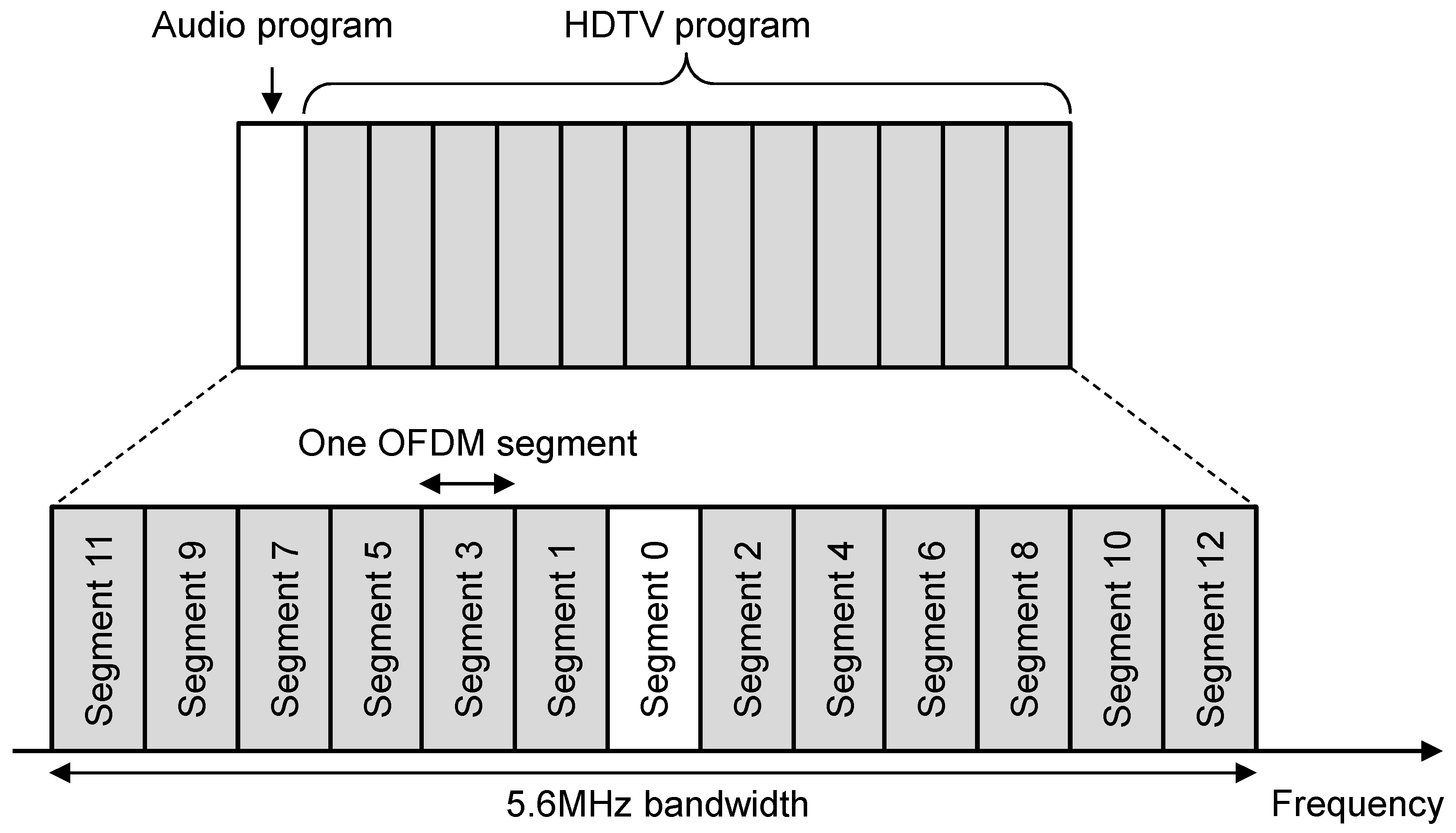
Orthogonal frequency division multiplexing (OFDM) is a multi-carrier technique that achieves a higher spectrum efficiency by using minimally spaced orthogonal subcarriers without increasing the implementation complexity. The success of OFDM is witnessed by its adoption into a lot of international digital television terrestrial broadcasting (DTTB) standards, including digital television/terrestrial multimedia broadcasting (DTMB), advanced television systems committee (ATSC) 3.0, digital video broadcasting-terrestrial-second generation (DVB-T2), and integrated services digital broadcasting-terrestrial (ISDB-T) [1,2,3,4]. Although many DTTB standards share a common OFDM framework, different technical features could be found [5,6]. The unique feature in ISDB-T is the use of band segmented transmission OFDM (BST-OFDM) to support different services and applications. A fundamental feature of BST-OFDM is the capability of using different coding and modulation schemes in one or more OFDM segments, which leads to the basis of hierarchical transmission [4,5,6]. In BST-OFDM, the entire band is equally divided into 13 segments with the same bandwidth, making it possible to transmit an HDTV program by combining 12 segments. Moreover, it is possible for an audio program to be received using one segment.

Besides several advantageous features, the OFDM system has some major problems that must be resolved. One of the major weakness of OFDM is its sensitivity to carrier frequency offset (CFO) and sampling frequency offset (SFO) which are caused by the mismatch between transmitter and receiver oscillators [7,8]. If not accurately estimated and compensated, the CFO and SFO can destroy the orthogonality among the subcarriers, leading to performance loss at the OFDM receiver [9,10]. In the literature, several types of pilot-aided algorithms have been proposed to perform the joint estimation of CFO and SFO, including maximum likelihood (ML) and linear least-squares (LS) strategies [11,12,13,14,15,16,17,18,19,20,21,22,23]. The joint ML estimation scheme needs a two-dimensional search to obtain the exact estimation of CFO and SFO. Due to prohibitively high computational processing, a practical implementation of ML approaches developed in [12,13,14] may become unrealistic. To account for this issue, significant attention has been paid to a simplified joint estimation of CFO and SFO using one-dimensional search or closed-form solution [15,16,17,18,19,20,21,22,23]. Specifically, estimation of the CFO and SFO for an unknown channel’s frequency response (CFR) is first reported in [15], which is based on the phase differences between the equidistant pilot subcarriers over two consecutive OFDM symbols. In [16], the decision-directed estimation of CFO and SFO without the use of pilots is presented, which increases the computational complexity and suffers from error propagation. Alternative pilot-aided estimation method is proposed in [17], applying the LS regression in the estimation of a linear combination of the CFO and SFO. In [18,19], the estimates over all the pilot-subcarriers are weighted using the frequency-domain channel estimates to improve the estimation accuracy. A suboptimal ML-oriented method is proposed in [20], where the joint estimation of the CFO and SFO is performed in a decoupled manner such that only one-dimensional search is needed. Similarly, the works in [21,22] propose replacing the two-dimensional search of [13] with a decoupled estimation scheme that is composed of closed-form estimation of the CFO and an approximate ML estimation for the SFO. The estimation method studied in [23] is based on a polynomial approximation for the ML cost function and its performance comes close to ML performance without resorting to an exhaustive search.

In the ISDB-T system, various types of pilot symbols such as scattered pilot (SP), continuous pilot (CP), transmission and multiplexing configuration control (TMCC), and auxiliary channel (AC) are provided for the purpose of synchronization. Since the number of available CPs is very small and some pilot information is not revealed until the TMCC information is decoded in the ISDB-T system, a direct application of the conventional joint LS estimation scheme [17,18,19] to the ISDB-T system gives rise to the loss in estimation accuracy. In particular, the numbers of CP and SP are changed according to which modulation is used in each segment. Therefore, it is of importance to make necessary changes to the conventional estimation strategy. For the purpose of accommodating the segment format, the estimation schemes [17,18,19] can be modified to utilize information-conveying TMCC control signals, which are present in an equal number regardless of a segment type, instead of the limited number of explicit pilots.

In this paper, we propose an efficient joint estimation of CFO ad SFO in the BST-OFDM based HDTV broadcast system without relying on a priori knowledge of segment type. To end this, the proposed joint LS estimation of CFO and SFO uses information-bearing TMCC signals that are commonly present irrespective of a segment type. Using the repeated nature of TMCC signals to discard the phase ambiguity before decoding TMCC information, the proposed estimation scheme can be a good solution for reliable estimation of frequency offsets. We confirm via numerical simulations that the proposed joint estimation scheme has a comparable performance to the conventional estimation scheme in spite of using information-bearing TMCC signals in a blind manner.

The remainder of this paper is organized as follows. A description of signal models adopted in this paper is presented in Section 2. In Section 3, the conventional joint LS estimation of CFO and SFO is discussed, resulting in some limitations when applied to the ISDB-T system. In Section 4, the effective joint LS estimation of CFO and SFO in the ISDB-T system using TMCC signals is suggested and its mean squared error (MSE) is derived. Section 5 presents the simulation results that verify the reliable operation of the proposed joint LS estimation scheme. Conclusions are drawn in Section 6.

2. System Model

In this paper, we consider an OFDM system using N-point inverse fast Fourier transform (IFFT) of size N. One OFDM symbol comprises $N_u<N$ non-zero subcarriers, and remnant $N-N_u$ subcarriers are assumed to be zero-inserted. After IFFT operation, the time-domain signal can be generated and a guard interval (GI) with a length of $N_g$ is inserted at the front of OFDM symbols in order to remove both inter-symbol interference (ISI) and inter-carrier interference (ICI). The l-th transmitted time domain signal can be given by

$$\begin{array}{cc}\hfill x_l\left(n\right)& =\sum _{k=0}^{N-1}{X}_l\left(k\right)e^{j2\pi kn/N},n=-N_g,N_g+1,\cdots ,N-1,\hfill \end{array}$$

(1)

where $X_l\left(k\right)$ is the symbol transmitted at the k-th subcarrier. Consequently, the effective duration of one OFDM symbol is $N_s{T}_s$, where $T_s$ is the sample time interval and $N_s=N+N_g$. Since our focus is on the post-FFT frequency synchronization, it is assumed that the coarse symbol timing offset (STO) and frequency offset estimation has been performed at the pre-FFT stage. Since many accurate coarse estimation schemes were studied in the literature [24,25], it is reasonable to assume that residual STO, CFO, and SFO are small enough after pre-FFT synchronization stage. Let ${\Delta }_c$ be the normalized CFO by the subcarrier spacing ${\Delta }_f=1/N{T}_s$ and ${\Delta }_s$ be the normalized SFO by the sampling frequency interval $1/T_s$

After IFFT, the received frequency-domain signal can be represented as [20,21,22,23]

$$\begin{array}{cc}\hfill R_l\left(k\right)& =\alpha \left(k\right)H_l\left(k\right)X_l\left(k\right)e^{-j2\pi k{\Delta }_{\tau }/N}{e}^{j2\pi \phi \left(k\right)(l{N}_s+N_g)/N}+C_l\left(k\right)+Z_l\left(k\right),\hfill \end{array}$$

(2)

where $\phi \left(k\right)={\Delta }_c+k{\Delta }_s$, $\alpha \left(k\right)$ is an amplitude attenuation incurred by $\phi \left(k\right)$, $H_l\left(k\right)$ is the CFR with variance ${\sigma }_H^2$, ${\Delta }_{\tau }$ is the residual STO, $Z_l\left(k\right)$ is the zero-mean additive white Gaussian noise (AWGN) with variance ${\sigma }_Z^2$, and $C_l\left(k\right)$ is the frequency–offset-induced ICI with variance ${\sigma }_C^2$. In (2), $\alpha \left(k\right)$ and $C_l\left(k\right)$ can be expressed as

$$\begin{array}{c}\hfill \alpha \left(k\right)=\frac{sin\left(\pi \right(\phi \left(k\right))}{Nsin\left(\pi \phi \right(k)/N)}\end{array}$$

(3)

and

$$\begin{array}{cc}\hfill C_l\left(k\right)& =\sum _{n=0,n\ne k}^{N-1}{H}_l\left(n\right)X_l\left(n\right)e^{j2\pi \phi \left(n\right)(l{N}_s+N_g)/N}\frac{sin\left(\pi \right(\phi \left(n\right)+n-k\left)\right)}{Nsin\left(\pi \right(\phi \left(n\right)+n-k)/N)}{e}^{j\pi (N-1)\left(\phi \right(n)+n-k)N}.\hfill \end{array}$$

(4)

Assuming that $X_l\left(n\right)$ are statistically independent for different n’s and l’s, from the central limit theorem $C_l\left(k\right)$ is treated as a zero-mean Gaussian random variable with variance [20]

$$\begin{array}{cc}\hfill {\sigma }_C^2& =E_X{\sigma }_H^2\sum _{n=0,n\ne k}^{N-1}\frac{{sin}^2\left(\pi (\phi \left(n\right)+n-k)\right)}{N^2{sin}^2(\pi (\phi \left(n\right)+n-k)/N)},\hfill \end{array}$$

(5)

where $E_X={|X_l\left(k\right)|}^2$. Note that $\alpha \left(k\right)\approx 1$ and ${\sigma }_C^2\approx E_X{\sigma }_H^2{\Delta }_c^2{\pi }^2/3$ for typical values of ${\Delta }_c$ and ${\Delta }_s$ [9].

Figure 1 shows the assignment of an OFDM segment and program in the ISDB-T system. As shown in Figure 1, one ISDB-T channel consists of 13 OFDM segments and up to three hierarchical layers can be supported with respect to these segments. The audio program segment is positioned in the middle of the frequency band, which is called narrowband ISDB-T. The narrowband ISDB-T mode only uses single or triple OFDM segments, whereas the wide-band ISDB-T system contains up to 13 segments and supports HDTV service.

Table 1. Transmission parameters for ISDB-T [4].

Parameters	Mode 1	Mode 2	Mode 3
FFT size	2k	4k	8k
Bandwidth	5.575 MHz	5.573 MHz	5.572 MHz
Subcarrier spacing	3.968 kHz	1.984 kHz	0.992 kHz
Effective symbol duration	252 $\mathsf{\mu }$s	504 $\mathsf{\mu }$s	1008 $\mathsf{\mu }$s
Number of segments	13	13	13
Number of carriers per segments	108	216	432
Number of usable carriers	1405	2809	5617
Number of SP carriers	$9\times N_c$	$18\times N_c$	$36\times N_c$
Number of CP carriers	$N_d+1$	$N_d+1$	$N_d+1$
Number of TMCC carriers	$N_c+5\times N_d$	$2\times N_c+10\times N_d$	$4\times N_c+20\times N_d$
Number of AC1 carriers	26	52	104
Number of AC2 carriers	$4\times N_d$	$9\times N_d$	$19\times N_d$

summarizes the basic transmission parameters of each mode for ISDB-T, where $N_d$ and $N_c$ are the numbers in differential-modulation and coherent-modulation segments, respectively. One OFDM frame includes 204 OFDM symbols and pilot carriers. The pilot signals include SP, CP, TMCC, and AC. The SP is present only in coherent-modulation segments in order to estimate the channel, whereas the other pilots can be mainly used to acquire time and frequency synchronization. The TMCC signal, which is inserted in the same format independent of segment types, includes system control information like the segment type and transmission parameters that the receiver has to decode first. Since the TMCC is information-bearing, the frequency estimation schemes that rely on the explicit pilots such as CP and SP are thus not adequate in this case of using TMCC signals as pilot symbols.

3. Conventional Estimation Scheme

The Post-FFT synchronization is practically performed in the frequency domain by the use of uniformly distributed pilot symbols as studied in [20,21,22,23]. Although the ISDB-T system provides periodically distributed SPs for receiver synchronization, its location will be known after decoding TMCC signals. On the other hand, the presence of CPs in many broadcast systems [2,3,4] makes it possible to correlate two consecutive OFDM symbols. Considering non-periodically distributed property of CPs in the frequency direction, the frequency–offset estimation scheme performed on a per-subcarrier basis is appropriate for the ISDB-T system. Therefore, this paper considers a carrier-by-carrier estimation scheme [17,18,19] that relies on the continuous-type pilot such as CP. By assuming that $H_l\left(k\right)=H_{l+1}\left(k\right)$ and $\alpha \left(k\right)\approx 1$, one obtains a conjugate product across consecutive symbols as [20]

$$\begin{array}{cc}\hfill Y_l\left(k\right)& =R_l^{*}\left(k\right)R_{l+1}\left(k\right)\hfill \\ & =|H_l{\left(k\right)|}^2{X}_l^{*}\left(k\right)X_{l+1}\left(k\right)e^{j2\pi \phi \left(k\right)\rho }+{\widehat{C}}_l\left(k\right)+{\widehat{Z}}_l\left(k\right),\hfill \end{array}$$

(6)

where $\rho =N_s/N$, ${\widehat{C}}_l\left(k\right)$ is the combined ICI given by

$$\begin{array}{cc}\hfill {\widehat{C}}_l\left(k\right)& =H_l^{*}\left(k\right)X_l^{*}\left(k\right)C_{l+1}\left(k\right)e^{j2\pi k{\Delta }_{\tau }/N}{e}^{-j2\pi \phi \left(k\right)(l{N}_s+N_g)/N}\hfill \\ & +H_{l+1}\left(k\right)X_{l+1}\left(k\right)C_l^{*}\left(k\right)e^{-j2\pi k{\Delta }_{\tau }/N}{e}^{j2\pi \phi \left(k\right)((l+1)N_s+N_g)/N}+C_l^{*}\left(k\right)C_{l+1}\left(k\right)\hfill \end{array}$$

(7)

and ${\tilde{Z}}_l\left(k\right)$ is the combined AWGN given by

$$\begin{array}{cc}\hfill {\widehat{Z}}_l\left(k\right)& =H_l^{*}\left(k\right)X_l^{*}\left(k\right)Z_{l+1}\left(k\right)e^{j2\pi k{\Delta }_{\tau }/N}{e}^{-j2\pi \phi \left(k\right)(l{N}_s+N_g)/N}\hfill \\ & +H_{l+1}\left(k\right)X_{l+1}\left(k\right)Z_l^{*}\left(k\right)e^{-j2\pi k{\Delta }_{\tau }/N}{e}^{j2\pi \phi \left(k\right)((l+1)N_s+N_g)/N}\hfill \\ & +C_{l+1}\left(k\right)Z_l^{*}\left(k\right)+C_l^{*}\left(k\right)Z_{l+1}\left(k\right)+Z_l^{*}\left(k\right)Z_{l+1}\left(k\right).\hfill \end{array}$$

(8)

From [20], $C_l\left(k\right)$ behaves like zero-mean Gaussian noise with variance ${\sigma }_C^2$. Since $E\left\{C_l\left(k\right)\right\}=E\left\{Z_l\left(k\right)\right\}=0$, it immediately follows from (7) and (8) that $E\{{\widehat{C}}_l\left(k\right)\}=E\{{\widehat{Z}}_l\left(k\right)\}=0$.

If $X_l\left(k\right)$ and $X_{l+1}\left(k\right)$ are known pilots at the receiver, by averaging the conjugate product across the multiple pilot pairs, the pilot-compensated signal is obtained as

$$\begin{array}{cc}\hfill {\tilde{Y}}_l\left(k\right)& =\sum _{l=1}^{N_a}{Y}_l\left(k\right)X_l\left(k\right)X_{l+1}^{*}\left(k\right)\hfill \\ & =\sum _{l=1}^{N_a}{|H_l\left(k\right)|}^2{E}_X^2{e}^{j2\pi \phi \left(k\right)\rho }+\sum _{l=1}^{N_a}{\widehat{C}}_l\left(k\right)X_l\left(k\right)X_{l+1}^{*}\left(k\right)+\sum _{l=1}^{N_a}{\widehat{Z}}_l\left(k\right)X_l\left(k\right)X_{l+1}^{*}\left(k\right)\hfill \end{array}$$

(9)

and its argument can be expressed as

$$\begin{array}{cc}\hfill \arg \{{\tilde{Y}}_l\left(k\right)\}& =2\pi \phi \left(k\right)\rho +I_l\left(k\right)\hfill \\ & =2\pi ({\Delta }_c+k{\Delta }_s)\rho +I_l\left(k\right),\hfill \end{array}$$

(10)

where $\arg \left\{x\right\}$ is the radian phase angle of the complex number x, $I_l\left(k\right)$ is the appropriate AWGN plus ICI contribution after taking an argument, and $N_a$ is the number of averaging used for mitigating interferences. Note that the effect of residual STO is cancelled out in the second term of the right-hand side (RHS) in (6) after conjugate operation because the phase rotation due to ${\Delta }_{\tau }$ is not a function of time inedex l. Since $\phi \left(k\right)$ is a linear function of ${\Delta }_c$ and ${\Delta }_s$ in (10), the LS estimates of ${\Delta }_c$ and ${\Delta }_s$ are computed as follows [17,18,19]:

$$\begin{array}{cc}\hfill {\widehat{\Delta }}_c& =\frac{1}{2\pi \rho N_f}\sum _{i=1}^{N_f}\arg \{{\tilde{Y}}_l\left(k_i\right)\}\hfill \\ & ={\Delta }_c+\frac{1}{2\pi \rho N_f}\sum _{i=1}^{N_f}{I}_l\left(k_i\right)+\frac{{\Delta }_s}{N_f}\sum _{i=1}^{N_f}{k}_i\hfill \end{array}$$

(11)

and

$$\begin{array}{cc}\hfill {\widehat{\Delta }}_s& =\frac{1}{2\pi \rho M_f}\sum _{i=1}^{N_f}{k}_i\arg \{{\tilde{Y}}_l\left(k_i\right)\}\hfill \\ & ={\Delta }_c+\frac{1}{2\pi \rho M_f}\sum _{i=1}^{N_f}{k}_i{I}_l\left(k_i\right)+\frac{{\Delta }_c}{M_f}\sum _{i=1}^{N_f}{k}_i,\hfill \end{array}$$

(12)

where $N_f$ is the number of CPs, $k_i$ is the index of the i-th CP subcarrier, the last terms of the RHS are the additional interference caused by the use of non-symmetrically distributed CPs, and

$$\begin{array}{cc}\hfill M_f& =\sum _{i=1}^{N_f}{k}_i^2.\hfill \end{array}$$

(13)

As reported in the literature [17,18,19], the drawback of LS estimation scheme is that its performance is strongly influenced by the noise under low signal-to-noise ratio (SNR). Since the ISDB-T system has no sufficient CPs for synchronization, it gives rise to a significant loss in estimation accuracy of (11) and (12). To overcome such a problem, an information-carrying TMCC signal can be considered as pilot symbols for the synchronization purpose.

4. Proposed Estimation Scheme

In this section, we present an effective joint LS estimation of CFO and SFO in the ISDB-T system without decoding TMCC signals. Since the same TMCC signals are transmitted by means of multiple carriers, such a repetition property can be incorporated for blind frequency–offset estimation. To show the effectiveness of the joint LS estimation scheme, the MSE performance is theoretically analyzed in the BST-OFDM context.

4.1. Algorithm Description

The number and position of TMCC subcarriers are changed in accordance with which modulation is being used in ISDB-T segments. Until the segment format is identified, which is completed after TMCC decoding, some TMCC subcarriers are unknown. Fortunately, there are common TMCC signals regardless of the segment format in the ISDB-T system, which is transmitted by means of the differential BPSK (DBPSK) modulation. Hence, the differential relation ${\overline{X}}_l\left(k\right)=X_l^{*}\left(k\right)X_{l+1}\left(k\right)=\pm {|X_l\left(k\right)|}^2$ is the same for all TMCC subcarrier positions. In order to remove its corresponding phase ambiguity, the product across adjacent pilot subcarriers $k_i$ and $k_{i+1}$ can be used instead of multiplying known pilots to $Y_l\left(k_i\right)$ as done in the conventional approach (9). With the above properties in mind, the phase-compensated signal is defined as follows:

$$\begin{array}{cc}\hfill {\overline{Y}}_l\left(k_i\right)& =\sum _{l=1}^{N_a}{Y}_l\left(k_i\right)Y_l\left(k_{i+1}\right)\hfill \\ & =\sum _{l=1}^{N_a}|H_l\left(k_i\right){|}^2{|H_l\left(k_{i+1}\right)|}^2{\overline{X}}_l\left(k_i\right){\overline{X}}_l\left(k_{i+1}\right)e^{j2\pi \overline{\phi }\left(k_i\right)\rho }+\sum _{l=1}^{N_a}{\overline{C}}_l\left(k_i\right)+\sum _{l=1}^{N_a}{\overline{Z}}_l\left(k_i\right),i=1,2,\cdots ,N_p-1,\hfill \end{array}$$

(14)

where $N_p$ is the number of common TMCC signals, $\overline{\phi }\left(k\right)=2{\Delta }_c+(k_i+k_{i+1}){\Delta }_s$, ${\overline{C}}_l\left(k_i\right)$ is the combined zero-mean ICI given by

$$\begin{array}{cc}\hfill {\overline{C}}_l\left(k_i\right)& =|H_l\left(k_i\right){|}^2{X}_l^{*}\left(k_i\right)X_{l+1}\left(k_i\right){\widehat{C}}_l\left(k_{i+1}\right)e^{j2\pi \phi \left(k_i\right)\rho }\hfill \\ & +|H_l\left(k_{i+1}\right){|}^2{X}_l^{*}\left(k_{i+1}\right)X_{l+1}\left(k_{i+1}\right){\widehat{C}}_l\left(k_i\right)e^{j2\pi \phi \left(k_{i+1}\right)\rho }+{\widehat{C}}_l\left(k_i\right){\widehat{C}}_l\left(k_{i+1}\right)\hfill \end{array}$$

(15)

and ${\overline{Z}}_l\left(k_i\right)$ is the zero-mean AWGN contribution given by

$$\begin{array}{cc}\hfill {\overline{Z}}_l\left(k_i\right)& =|H_l\left(k_i\right){|}^2{X}_l^{*}\left(k_i\right)X_{l+1}\left(k_i\right){\widehat{Z}}_l\left(k_{i+1}\right)e^{j2\pi \phi \left(k_i\right)\rho }\hfill \\ & +|H_l\left(k_{i+1}\right){|}^2{X}_l^{*}\left(k_{i+1}\right)X_{l+1}\left(k_{i+1}\right){\widehat{Z}}_l\left(k_i\right)e^{j2\pi \phi \left(k_{i+1}\right)\rho }\hfill \\ & +{\widehat{C}}_l\left(k_i\right){\widehat{Z}}_l\left(k_{i+1}\right)+{\widehat{C}}_l\left(k_{i+1}\right){\widehat{Z}}_l\left(k_i\right)+{\widehat{Z}}_l\left(k_i\right){\widehat{Z}}_l\left(k_{i+1}\right).\hfill \end{array}$$

(16)

Recognizing the fact that the TMCC information is common to all TMCC subcarriers and is DBPSK modulated, $\arg \{{\overline{X}}_l\left(k_i\right)\}=\arg \{{\overline{X}}_l\left(k_{i+1}\right)\}$ for all pilot subcarrier indices i’s during the l-th period. Therefore, ${\overline{X}}_l\left(k_i\right){\overline{X}}_l\left(k_{i+1}\right)=E_X^2$ such that

$$\begin{array}{cc}\hfill {\overline{Y}}_l\left(k_i\right)& =\sum _{l=1}^{N_a}|H_l\left(k_i\right){|}^2{|H_l\left(k_{i+1}\right)|}^2{E}_X^2{e}^{j2\pi \overline{\phi }\left(k_i\right)\rho }+\sum _{l=1}^{N_a}{\overline{C}}_l\left(k_i\right)+\sum _{l=1}^{N_a}{\overline{Z}}_l\left(k_i\right),i=1,2,\cdots ,N_p-1,\hfill \end{array}$$

(17)

where $E_X={|X_l\left(k\right)|}^2$ is the TMCC symbol energy. The property (17) is the basis of the CFO and SFO estimation in the proposed blind method, which is only valid for binary-modulated signals.

Since $E\{{\overline{C}}_l\left(k_i\right)\}=E\{{\overline{Z}}_l\left(k_i\right)\}=0$, it follows that

$$\begin{array}{cc}\hfill \arg \left\{E\left\{{\overline{Y}}_l\left(k_i\right)\right\}\right\}& =2\pi \overline{\phi }\left(k\right)\rho \hfill \\ & =4\pi {\Delta }_c\rho +2\pi (k_i+k_{i+1}){\Delta }_s\rho .\hfill \end{array}$$

(18)

When compared to (10), it is obvious from (18) that the amount of phase rotation of ${\overline{Y}}_l\left(k_i\right)$ due to frequency offsets is approximately twice, which leads to the robustness to the noise. On the contrary, one can see from (9) and (17) that the noise contribution in (17) becomes approximately four times as large as that in (9). Recalling from (18) that $\overline{\phi }\left(k\right)=2{\Delta }_c+(k_i+k_{i+1}){\Delta }_s$ is a linear function of ${\Delta }_c$ and ${\Delta }_s$, the proposed joint estimation of CFO and SFO can be constructed in the LS manner as follows:

$$\begin{array}{cc}\hfill {\widehat{\Delta }}_c& =\frac{1}{4\pi \rho (N_p-1)}\sum _{i=1}^{N_p-1}\arg \left\{{\overline{Y}}_l\left(k_i\right)\right\}\hfill \end{array}$$

(19)

and

$$\begin{array}{cc}\hfill {\widehat{\Delta }}_s& =\frac{1}{2\pi \rho M_p}\sum _{i=1}^{N_p-1}(k_i+k_{i+1})\arg \left\{{\overline{Y}}_l\left(k_i\right)\right\},\hfill \end{array}$$

(20)

where

$$\begin{array}{cc}\hfill M_p& =\sum _{i=1}^{N_p-1}{(k_i+k_{i+1})}^2.\hfill \end{array}$$

(21)

It is worthwhile to mention that the number of common TMCC signals $N_p=13$ for 2k mode, $N_p=26$ for 4k mode, and $N_p=52$ for 8k mode [4]. Since the number of the common TMCC subcarriers may be insufficient in the case of 2k mode, we adopt the averaged estimation over $N_a$ symbol intervals as in (14). Of course, the cost to be paid for using this averaging approach is an increase in computational complexity.

For notational convenience, (17) is rearranged into

$$\begin{array}{cc}\hfill {\overline{Y}}_l\left(k_i\right)& =\sum _{l=1}^{N_a}|H_l\left(k_i\right){|}^2{|H_l\left(k_{i+1}\right)|}^2{E}_X^2{e}^{j2\pi \overline{\phi }\left(k_i\right)\rho }\left[1+\frac{{\sum }_{l=1}^{N_a}\{{\overline{C}}_l\left(k_i\right)+{\overline{Z}}_l\left(k_i\right)\}{e}^{-j2\pi \overline{\phi }\left(k\right)\rho }}{{\sum }_{l=1}^{N_a}|H_l\left(k_i\right){|}^2{|H_l\left(k_{i+1}\right)|}^2{E}_X^2}\right].\hfill \end{array}$$

(22)

Under the high SNR condition and pilot boosting, the argument of ${\overline{Y}}_l\left(k_i\right)$ can be well approximated by

$$\begin{array}{c}\hfill \arg \left\{{\overline{Y}}_l\left(k_i\right)\right\}\approx 2\pi \overline{\phi }\left(k_i\right)\rho +\frac{{\sum }_{l=1}^{N_a}{\tilde{C}}_l^Q\left(k_i\right)+{\sum }_{l=1}^{N_a}{\tilde{Z}}_l^Q\left(k_i\right)}{{\sum }_{l=1}^{N_a}|H_l\left(k_i\right){|}^2{|H_l\left(k_{i+1}\right)|}^2{E}_X^2},\end{array}$$

(23)

where $X^Q$ be the quadrature component of X, and ${\tilde{C}}_l\left(k\right)={\overline{C}}_l\left(k\right)e^{-j2\pi \overline{\phi }\left(k\right)\rho }$ and ${\tilde{Z}}_l\left(k\right)={\overline{Z}}_l\left(k\right)e^{-j2\pi \overline{\phi }\left(k\right)\rho }$ are statistically equivalent to ${\overline{C}}_l\left(k\right)$ and ${\overline{Z}}_l\left(k\right)$, respectively. From (19)–(23), it is easy to find that the estimation error of CFO and SFO is calculated by

$$\begin{array}{cc}\hfill {\widehat{\Delta }}_c-{\Delta }_c& =\frac{1}{4\pi \rho (N_p-1)E_X^2}\sum _{i=1}^{N_p-1}\frac{{\sum }_{l=1}^{N_a}{\tilde{C}}_l^Q\left(k_i\right)+{\sum }_{l=1}^{N_a}{\tilde{Z}}_l^Q\left(k_i\right)}{{\sum }_{l=1}^{N_a}|H_l\left(k_i\right){|}^2{|H_l\left(k_{i+1}\right)|}^2}+I\left({\Delta }_s\right)\hfill \end{array}$$

(24)

and

$$\begin{array}{cc}\hfill {\widehat{\Delta }}_s-{\Delta }_s& =\frac{1}{2\pi \rho M_p{E}_X^2}\sum _{i=1}^{N_p-1}(k_i+k_{i+1})\frac{{\sum }_{l=1}^{N_a}{\tilde{C}}_l^Q\left(k_i\right)+{\sum }_{l=1}^{N_a}{\tilde{Z}}_l^Q\left(k_i\right)}{{\sum }_{l=1}^{N_a}|H_l\left(k_i\right){|}^2{|H_l\left(k_{i+1}\right)|}^2}+I\left({\Delta }_c\right),\hfill \end{array}$$

(25)

where $I\left({\Delta }_s\right)$ and $I\left({\Delta }_c\right)$ are the biases incurred from non-equidistant TMCC subcarriers given by

$$\begin{array}{cc}\hfill I\left({\Delta }_s\right)& =\frac{{\Delta }_s}{2(N_p-1)}\sum _{i=1}^{N_p-1}(k_i+k_{i+1})\hfill \end{array}$$

(26)

and

$$\begin{array}{cc}\hfill I\left({\Delta }_c\right)& =\frac{2{\Delta }_c}{M_p}\sum _{i=1}^{N_p-1}(k_i+k_{i+1}).\hfill \end{array}$$

(27)

As shown in (26) and (27), $I\left({\Delta }_s\right)$ and $I\left({\Delta }_c\right)$ are functions of frequency offsets and pilot indices so that they are constant as the SNR increases. Since frequency offsets are sufficiently small during the post-FFT tracking mode and TMCC subcarriers are evenly distributed over the entire transmission spectrum, $I^2\left({\Delta }_s\right)$ and $I^2\left({\Delta }_c\right)$ are insignificant as compared to the powers of their respective first terms in (24) and (25).

4.2. MSE Analysis

As a performance measure of the estimation scheme, we drive a closed-form expression of MSE of joint LS estimation in the frequency-selective fading channel. In our analysis, we assume that the channel is sufficiently frequency-selective such that the channel fading coefficients between neighboring subcarriers become uncorrelated. Having in mind that $E\{{\tilde{C}}_l^Q\left(k_i\right)\}=E\{{\tilde{Z}}_l^Q\left(k_i\right)\}=0$ and ${\tilde{C}}_l^Q\left(k_i\right)$ is statistically independent of ${\tilde{Z}}_l^Q\left(k_i\right)$, we obtain from (24)

$$\begin{array}{cc}\hfill E\left\{{\left|{\widehat{\Delta }}_c-{\Delta }_c\right|}^2\right\}& ={\left(\frac{1}{4\pi \rho (N_p-1)E_X^2}\right)}^2\sum _{i=1}^{N_p-1}E\left\{\frac{{\sum }_{l=1}^{N_a}{|{\tilde{C}}_l^Q\left(k_i\right)|}^2}{({\sum }_{l=1}^{N_a}|H_l\left(k_i\right){|}^2|H_l\left(k_{i+1}\right){{|}^2)}^2}\right\}\hfill \\ & +{\left(\frac{1}{4\pi \rho (N_p-1)E_X^2}\right)}^2\sum _{i=1}^{N_p-1}E\left\{\frac{{\sum }_{l=1}^{N_a}{|{\tilde{Z}}_l^Q\left(k_i\right)|}^2}{({\sum }_{l=1}^{N_a}|H_l\left(k_i\right){|}^2|H_l\left(k_{i+1}\right){{|}^2)}^2}\right\}+I^2\left({\Delta }_s\right).\hfill \end{array}$$

(28)

After substituting (15) to (28), we immediately establish

$$\begin{array}{cc}\hfill E\left\{\frac{{\sum }_{l=1}^{N_a}{|{\tilde{C}}_l^Q\left(k_i\right)|}^2}{({\sum }_{l=1}^{N_a}|H_l\left(k_i\right){|}^2|H_l\left(k_{i+1}\right){{|}^2)}^2}\right\}& =E_X^{2}E\left\{\frac{{\sum }_{l=1}^{N_a}|H_l\left(k_i\right){|}^4{|{\widehat{C}}_l^Q\left(k_{i+1}\right)|}^2}{({\sum }_{l=1}^{N_a}|H_l\left(k_i\right){|}^2|H_l\left(k_{i+1}\right){{|}^2)}^2}\right\}\hfill \\ & +E_X^{2}E\left\{\frac{{\sum }_{l=1}^{N_a}|H_l\left(k_{i+1}\right){|}^4{|{\widehat{C}}_l^Q\left(k_i\right)|}^2}{({\sum }_{l=1}^{N_a}|H_l\left(k_i\right){|}^2|H_l\left(k_{i+1}\right){{|}^2)}^2}\right\}\hfill \\ & +E\left\{\frac{{\sum }_{l=1}^{N_a}|{\widehat{C}}_l^Q\left(k_i\right){|}^2{|{\widehat{C}}_l^Q\left(k_{i+1}\right)|}^2}{({\sum }_{l=1}^{N_a}|H_l\left(k_i\right){|}^2|H_l\left(k_{i+1}\right){{|}^2)}^2}\right\}.\hfill \end{array}$$

(29)

Since the variance of ${\widehat{C}}_l\left(k\right)$ in (15) is ${\sigma }_{\widehat{C}}^2=2E_X{\sigma }_H^2{\sigma }_C^2+{\sigma }_C^4$, one can readily find that $E\{{\widehat{C}}_l^Q\left(k_i\right){|}^2|{\widehat{C}}_l^Q\left(k_{i+1}\right){|}^2\}={(E_X{\sigma }_H^2{\sigma }_C^2+{\sigma }_C^4/2)}^2$. Recalling from (5) that ${\sigma }_C^2\approx E_X{\sigma }_H^2{\Delta }_c^2{\pi }^2/3$ and pilot symbol is booted at $E_X=16/9$, the power of the last term of the RHS in (29) is very small compared to the powers of other terms; thereby, we can omit this term. Considering that the channel is time-invariant during $N_a$ symbol durations, after substituting (7) to (29), it can be calculated as

$$\begin{array}{cc}\hfill E\left\{\frac{{\sum }_{l=1}^{N_a}{|{\tilde{C}}_l^Q\left(k_i\right)|}^2}{({\sum }_{l=1}^{N_a}|H_l\left(k_i\right){|}^2|H_l\left(k_{i+1}\right){{|}^2)}^2}\right\}& =\frac{E_X^3{\sigma }_C^2}{N_a}\sum _{m=0}^{1}E\left\{\frac{1}{|H_l\left(k_{i+m}\right){|}^2}\right\}+\frac{E_X^2{\sigma }_C^4}{2N_a}\sum _{m=0}^{1}E\left\{\frac{1}{|H_l\left(k_{i+m}\right){|}^4}\right\}.\hfill \end{array}$$

(30)

It is obvious from (16) that the variance of ${\widehat{Z}}_l\left(k\right)$ is ${\sigma }_{\widehat{Z}}^2=2E_X{\sigma }_H^2{\sigma }_Z^2+2{\sigma }_C^2{\sigma }_Z^2+{\sigma }_Z^4$. Therefore, the variances of ${\widehat{C}}_l\left(k_i\right){\widehat{Z}}_l\left(k_{i+1}\right)$ and ${\widehat{Z}}_l\left(k_i\right){\widehat{Z}}_l\left(k_{i+1}\right)$ are very small compared to the powers of other terms in (16). In a similar way, neglecting these terms leads to

$$\begin{array}{cc}\hfill E\left\{\frac{{\sum }_{l=1}^{N_a}{|{\tilde{Z}}_l^Q\left(k_i\right)|}^2}{({\sum }_{l=1}^{N_a}|H_l\left(k_i\right){|}^2|H_l\left(k_{i+1}\right){{|}^2)}^2}\right\}& =E_X^{2}E\left\{\frac{{\sum }_{l=1}^{N_a}|H_l\left(k_i\right){|}^4{|{\widehat{Z}}_l^Q\left(k_{i+1}\right)|}^2}{({\sum }_{l=1}^{N_a}|H_l\left(k_i\right){|}^2|H_l\left(k_{i+1}\right){{|}^2)}^2}\right\}\hfill \\ & +E_X^{2}E\left\{\frac{{\sum }_{l=1}^{N_a}|H_l\left(k_{i+1}\right){|}^4{|{\widehat{Z}}_l^Q\left(k_i\right)|}^2}{({\sum }_{l=1}^{N_a}|H_l\left(k_i\right){|}^2|H_l\left(k_{i+1}\right){{|}^2)}^2}\right\},\hfill \end{array}$$

(31)

which is further derived as

$$\begin{array}{cc}\hfill E\left\{\frac{{\sum }_{l=1}^{N_a}{|{\tilde{Z}}_l^Q\left(k_i\right)|}^2}{({\sum }_{l=1}^{N_a}|H_l\left(k_i\right){|}^2|H_l\left(k_{i+1}\right){{|}^2)}^2}\right\}& =\frac{E_X^3{\sigma }_Z^2}{N_a}\sum _{m=0}^{1}E\left\{\frac{1}{|H_l\left(k_{i+m}\right){|}^2}\right\}\hfill \\ & +\frac{E_X^2}{2N_a}(2{\sigma }_C^2{\sigma }_Z^2+{\sigma }_Z^4)\sum _{m=0}^{1}E\left\{\frac{1}{|H_l\left(k_{i+m}\right){|}^4}\right\}.\hfill \end{array}$$

(32)

Since the probability density function of $x=|H_l{\left(k\right)|}^2$ in (32) is a central chi-square distribution with two degrees of freedom denoted by $f_H\left(x\right)={\sigma }_H^{-2}{e}^{-x/{\sigma }_H^2}$, it is effortlessly obtained that for any positive integer n

$$\begin{array}{cc}\hfill E\left\{\frac{1}{|H_l\left(k_{i+m}\right){|}^{2n}}\right\}& ={\int }_{p_{min}}^{\infty }\frac{1}{x^n{\sigma }_H^2}{e}^{-x/{\sigma }_H^2}dx\hfill \\ & ={(-1)}^n\frac{1}{(n-1)!{\left({\sigma }_H^2\right)}^n}{E}_i(-p_{min}/{\sigma }_H^2)\hfill \\ & +\frac{e^{-p_{min}/{\sigma }_H^2}}{p_{min}^{n-1}{\sigma }_H^2}\sum _{k=0}^{n-2}\frac{{(-1)}^k{(p_{min}/{\sigma }_H^2)}^k}{n(n-1)\cdots (n-k)},m=0,1,\hfill \end{array}$$

(33)

where $E_i(-x)=-{\int }_x^{\infty }{e}^{-t}/tdt$. From (30) and (32), one can see that they are not indepedent of index i. Therefore, plugging (30) and (32) into (28), we have

$$\begin{array}{c}E\left\{{\left|{\widehat{\Delta }}_c-{\Delta }_c\right|}^2\right\}\hfill \\ =\frac{1}{16{\pi }^2{\rho }^2{N}_a(N_p-1)}\left(\frac{{\sigma }_Z^2}{E_X}\sum _{m=0}^{1}E\left\{\frac{1}{|H_l\left(k_{i+m}\right){|}^2}\right\}+\frac{2{\sigma }_C^2{\sigma }_Z^2+{\sigma }_Z^4}{2E_X^2}\sum _{m=0}^{1}E\left\{\frac{1}{|H_l\left(k_{i+m}\right){|}^4}\right\}\right)\hfill \\ +\frac{1}{16{\pi }^2{\rho }^2{N}_a(N_p-1)}\left(\frac{{\sigma }_C^2}{E_X}\sum _{m=0}^{1}E\left\{\frac{1}{|H_l\left(k_{i+m}\right){|}^2}\right\}+\frac{{\sigma }_C^4}{2E_X^2}\sum _{m=0}^{1}E\left\{\frac{1}{|H_l\left(k_{i+m}\right){|}^4}\right\}\right)+I^2\left({\Delta }_s\right).\hfill \end{array}$$

(34)

Using (33), after some manipulations, the final MSE of the LS CFO estimate can be obtained by

$$\begin{array}{cc}\hfill E\left\{{\left|{\widehat{\Delta }}_c-{\Delta }_c\right|}^2\right\}& =\frac{1}{8{\pi }^2{\rho }^2{N}_a(N_p-1)}\left(\frac{{\lambda }_1}{{\gamma }_z}+\frac{{\lambda }_2}{{\gamma }_z{\gamma }_c}+\frac{{\lambda }_2}{2{\gamma }_z^2}\right)\hfill \\ & +\frac{1}{8{\pi }^2{\rho }^2{N}_a(N_p-1)}\left(\frac{{\lambda }_1}{{\gamma }_c}+\frac{{\lambda }_2}{2{\gamma }_c^2}\right)+I^2\left({\Delta }_s\right),\hfill \end{array}$$

(35)

where ${\lambda }_1=-E_i(-p_{min}/{\sigma }_H^2)$, ${\lambda }_2=E_i(-p_{min}/{\sigma }_H^2)+e^{-p_{min}/{\sigma }_H^2}/(p_{min}/{\sigma }_H^2)$, ${\gamma }_z={\sigma }_H^2{E}_X/{\sigma }_Z^2$ is the average SNR, and ${\gamma }_c={\sigma }_H^2{E}_X/{\sigma }_C^2$ is the average signal-to-ICI ratio. Similarly, the MSE of the SFO estimate can be conceptually given by

$$\begin{array}{cc}\hfill E\left\{{\left|{\widehat{\Delta }}_s-{\Delta }_s\right|}^2\right\}& ={\left(\frac{1}{2\pi \rho M_p{E}_X^2}\right)}^2\sum _{i=1}^{N_p-1}{(k_i+k_{i+1})}^{2}E\left\{\frac{{\sum }_{l=1}^{N_a}{|{\tilde{C}}_l^Q\left(k_i\right)|}^2}{({\sum }_{l=1}^{N_a}|H_l\left(k_i\right){|}^2|H_l\left(k_{i+1}\right){{|}^2)}^2}\right\}\hfill \\ & +{\left(\frac{1}{2\pi \rho M_p{E}_X^2}\right)}^2\sum _{i=1}^{N_p-1}{(k_i+k_{i+1})}^{2}E\left\{\frac{{\sum }_{l=1}^{N_a}{|{\tilde{Z}}_l^Q\left(k_i\right)|}^2}{({\sum }_{l=1}^{N_a}|H_l\left(k_i\right){|}^2|H_l\left(k_{i+1}\right){{|}^2)}^2}\right\}+I^2\left({\Delta }_c\right).\hfill \end{array}$$

(36)

Substituting (30) and (32) to (36) yields the final MSE of the SFO estimate as

$$\begin{array}{cc}\hfill E\left\{{\left|{\widehat{\Delta }}_s-{\Delta }_s\right|}^2\right\}& =\frac{1}{2{\pi }^2{\rho }^2{N}_a{M}_p}\left(\frac{{\lambda }_1}{{\gamma }_z}+\frac{{\lambda }_2}{{\gamma }_z{\gamma }_c}+\frac{{\lambda }_2}{2{\gamma }_z^2}\right)\hfill \\ & +\frac{1}{2{\pi }^2{\rho }^2{N}_a{M}_p}\left(\frac{{\lambda }_1}{{\gamma }_c}+\frac{{\lambda }_2}{2{\gamma }_c^2}\right)+I^2\left({\Delta }_c\right),\hfill \end{array}$$

(37)

where the first term of the RHS disappears as SNR increases and the other terms form an irreducible error floor caused by frequency offsets.

As a baseline for the performance of the estimators, we use the Cramer–Rao bound (CRB) for the estimates of ${\Delta }_c$ and ${\Delta }_s$, calculated assuming that the CFR is unknown and no averaging is used [20]

$$\begin{array}{cc}\hfill \mathrm{CRB}\left\{{\Delta }_c\right\}& =\frac{{\sigma }_Z^2}{4{\pi }^2{\rho }^2{N}_p{E}_X}·\frac{J\left(3\right)}{J\left(1\right)J\left(3\right)-J^2\left(2\right)}\hfill \end{array}$$

(38)

and

$$\begin{array}{cc}\hfill \mathrm{CRB}\left\{{\Delta }_s\right\}& =\frac{{\sigma }_Z^2}{4{\pi }^2{\rho }^2{N}_p{E}_X}·\frac{J\left(1\right)}{J\left(1\right)J\left(3\right)-J^2\left(2\right)},\hfill \end{array}$$

(39)

where $J\left(g\right)=(1/N_p){\sum }_{i=1}^{N_p}{k}_i^{g-1}{|H_l\left(k_i\right)|}^2$ for $g=1,2,3$.

4.3. Computational Complexity

Let us now consider the computational load of the estimation schemes. To make a parallel between the conventional and proposed estimation schemes, we consider the situation where the conventional scheme uses $N_f=N_p$ explicit pilots, although in practice the number of explicit CPs is very small compared to that of TMCC signals.

Table 2. The complexity of the joint estimation schemes.

Algorithm	Complex Multiplication	Real Multiplication	Real Addition
Conventional	$N_a{N}_f$	$4N_a{N}_f+N_f+2$	$2(N_f-1)$
Proposed	$N_a(2N_p-1)$	$N_p+1$	$2(N_p-1)$

shows the complexity of the conventional and proposed estimation schemes. The complexity of the estimation methods is compared with respect to the number of real floating point operations (flops). We assume that a complex multiplication is counted as six flops [26]. With this provision, the number of real flops needed to jointly get the estimate is $10N_a{N}_f+3N_f$ for the conventional scheme, whereas the proposed scheme requires $6N_a(2N_p-1)+3N_p-1$ real flops.

5. Simulation Results and Discussion

The performance of an OFDM system is evaluated with the ISDB-T transmission parameters summarized in Table 1 and the following parameter settings: a common carrier frequency of $f_c=800$ MHz, a sampling time of $T_s$ = 63/512 $\mathsf{\mu }$s, and GI ratio of 1/8 for all tramsmission modes [4]. The channel profile is the 6-tap Typical Urban defined in [27], where the amplitude of each tap is Rayleigh distributed such that a non-line-of-sight (NLOS) scenario is considered. In our simulations, Doppler effects due to mobility are not considered for the purpose of verifying the accuracy of MSE analysis. For fair comparison, we consider that $N_f=N_p$ for the conventional and proposed methods.

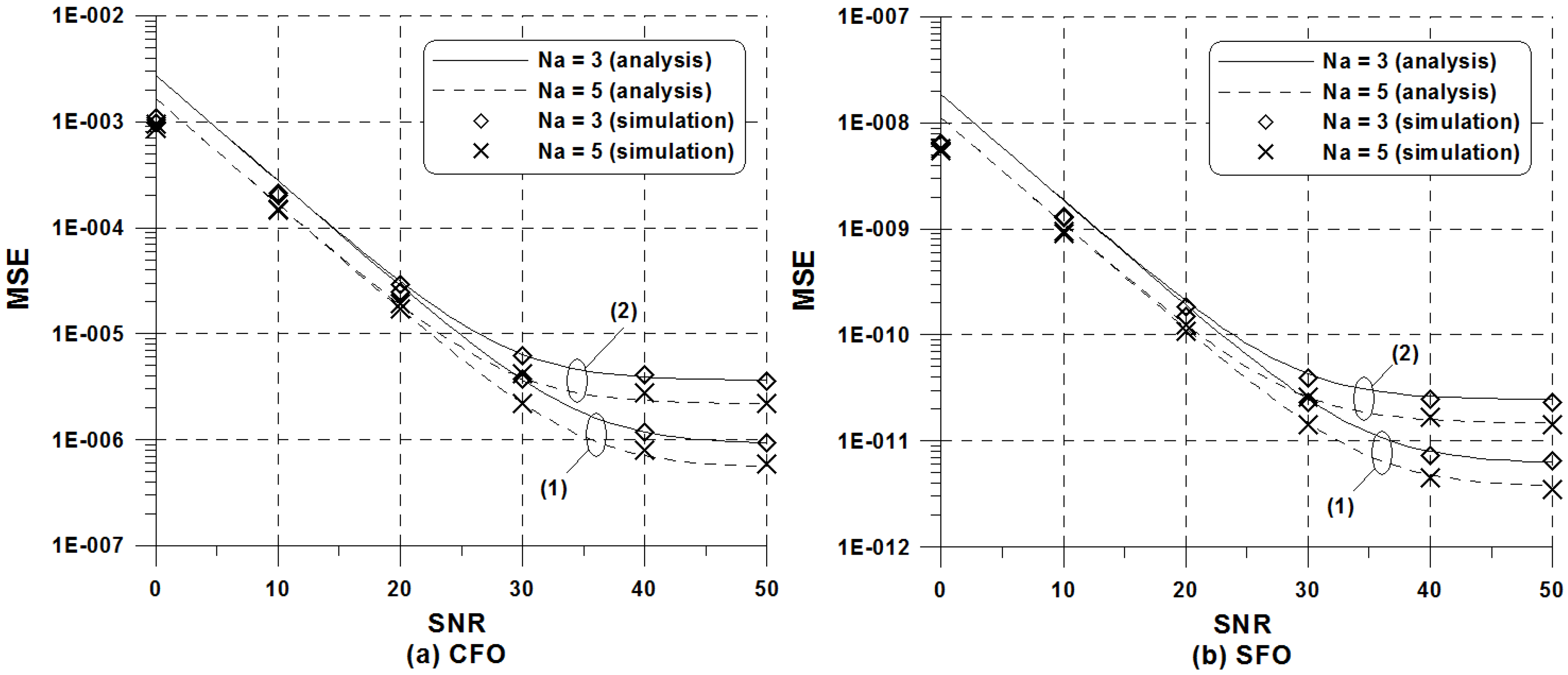
Figure 2 shows the MSE of the proposed joint LS estimator versus the number of averaging in the ISDB-T 2k mode. The probability of Rayleigh distributed random variable $|H_l\left(k\right)|$ exceeding a minimum level $p_{min}$ is $e^{-p_{min}/{\sigma }_H^2}$ such that the 99.9% level of Rayleigh fading could be achieved when $p_{min}/{\sigma }_H^2=-30$ dB, which is used to calculate the MSE in (35) and (37). It is observed that theoretical results closely match to the simulation results regardless of $N_a$ and frequency offsets. There is a small gap between the simulated and analytical curves at low SNR because of the approximation used in (23). As expected, one can see that the averaging strategy is an attractive solution to improve the estimation accuracy at the expense of computational complexity and processing delay. Nevertheless, the increase of frequency offsets leads to a severe irreducible error floor as the SNR grows.

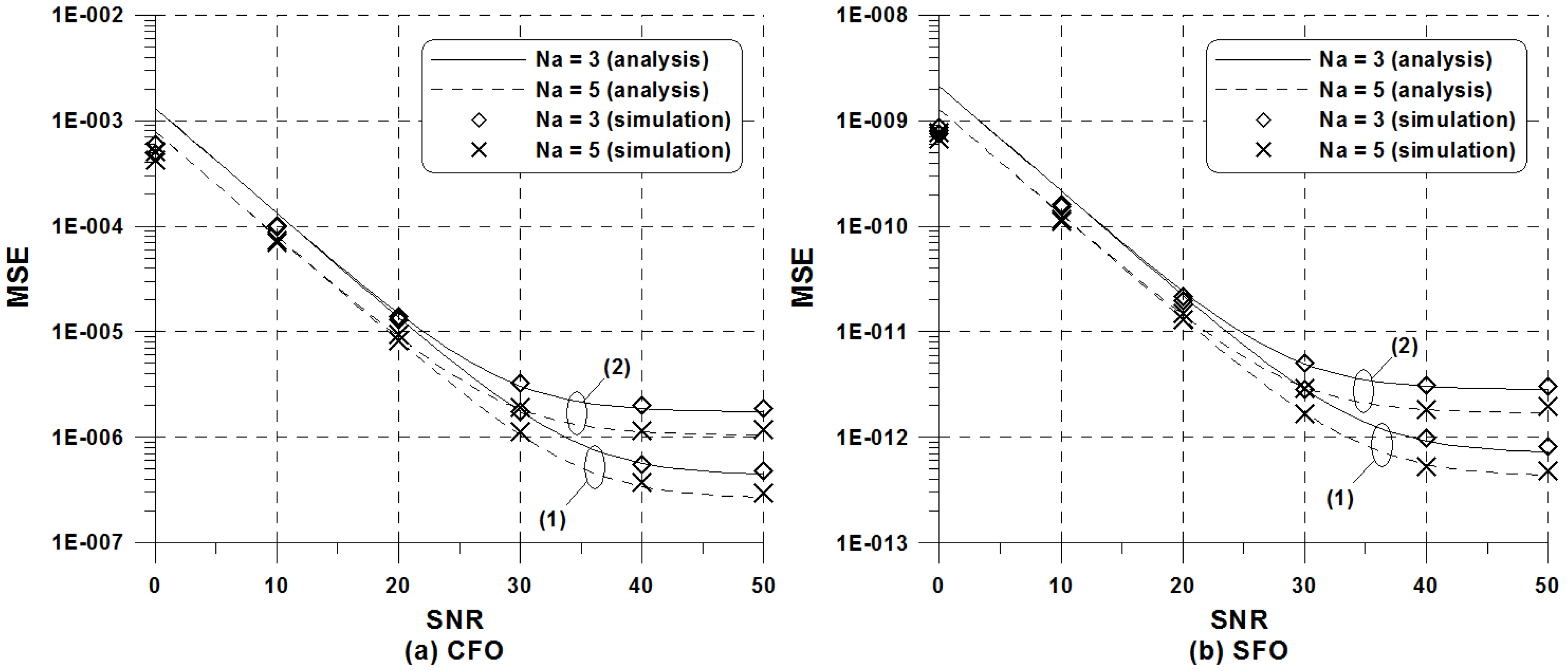
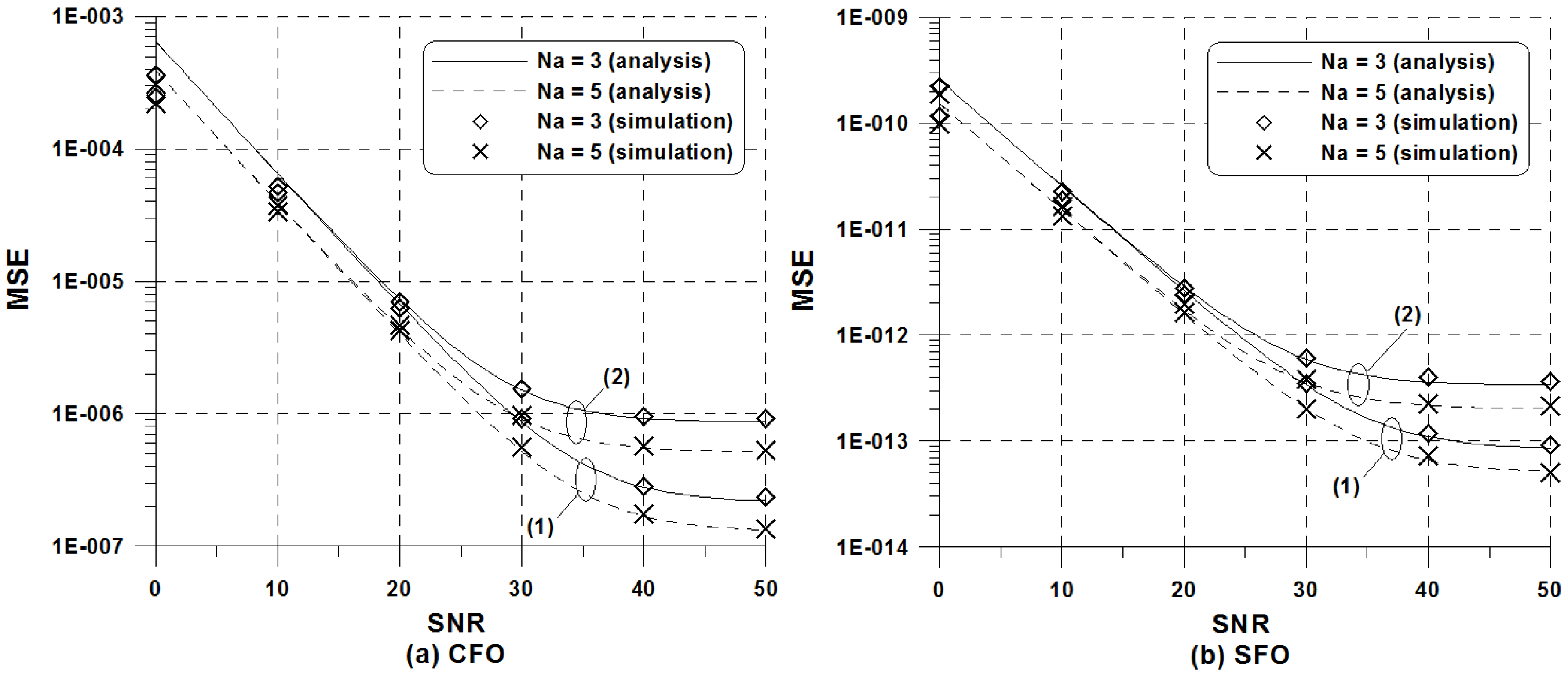
Figure 3 and Figure 4 illustrate the MSE of the proposed joint LS estimator versus $N_a$ in the ISDB-T 4k and 8k modes, respectively, under the same simulation scenarios to Figure 2. In these examples, $N_p=26$ for 4k mode and $N_p=52$ for 8k mode. Here, we can see a similar trend to that of Figure 2 where $N_p=13$ is used in 2k mode. It is evident that the large number of TMCC signals tends to give a more accurate match between the simulated and analytical curves. The more TMCC signals available in one OFDM symbol that can take part in the joint estimation of CFO and SFO, the better the ICI can be mitigated, as the ICI is similarly treated as AWGN.

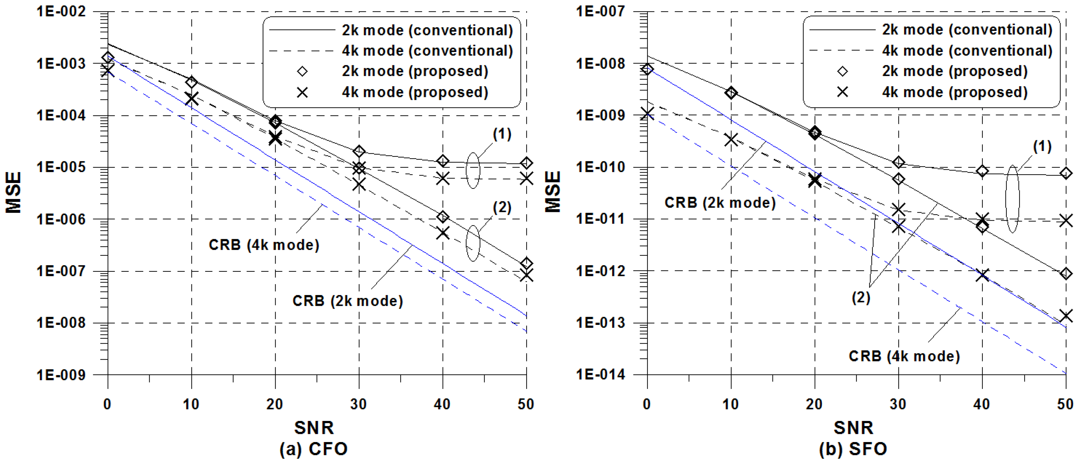
Figure 5 presents the MSE comparison between the conventional and proposed LS estimators when $N_a=1$, ${\Delta }_c=0.02$, and ${\Delta }_s=20$ ppm. The CRBs using (38) and (39) are also presented as a baseline reference. It can be seen that the MSE performance is the same for both schemes and all algorithms suffer from an error floor for higher SNR values, regardless of the transmission mode. In practice, the conventional joint LS estimation scheme cannot be directly applied to the ISDB-T system because of an unknown phase of TMCC signals, whereas the proposed estimation scheme resolves this problem using the repeated property of TMCC signals as done in (17). The performance difference between 2k and 4k modes becomes more visible in the case of SFO estimation. This is because the performance of the SFO estimation scheme relies on both the number and location of TMCC subcarriers as in (37), whereas the CFO estimation performance is dependent on only $N_p$. In order to examine the effect of bias caused by the use of non-uniformly distributed pilot, we also consider the scenario that there is no ICI. In this case, one can see that the bias of the proposed scheme is more significant than that of the conventional scheme at the high SNR. Regarding the number of flops when $N_a=1$, the proposed estimation scheme needs $15N_p-7$ real flops, whereas the conventional estimation scheme requires $13N_f$. Considering that $N_p=N_f$, the complexity of the proposed scheme is slightly increased by 11% and 13% in comparison with that of the conventional scheme considering 2k and 4k modes, respectively. In summary, we confirm that the information-carrying TMCC signal can be efficiently used for reliable joint LS estimation of CFO and SFO, achieving a satisfactory performance with moderate computational burden.

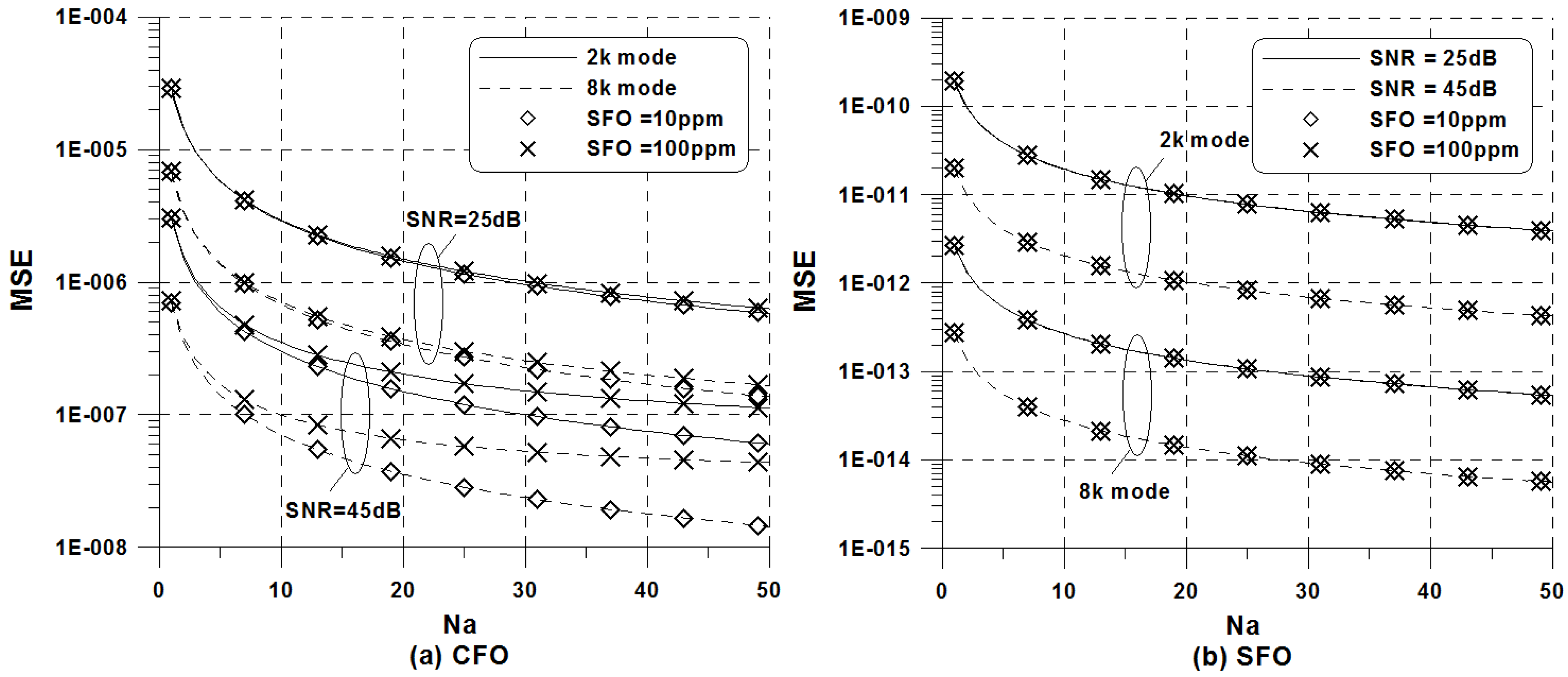
The impact of the parameter $N_a$ on the performance of the proposed joint LS estimation scheme is further investigated in Figure 6. The performance of the SFO estimator is not affected by the increase of SFO values, whereas the increased SFO leads to a severe error floor in the CFO estimation at high SNR. The reason for that primarily stems from the fact that the impact of $I\left({\Delta }_s\right)$ becomes more dominant compared to that of SFO-induced ICI at high SNR. In order to obtain the same MSE of the CFO regardless of SNR, approximately four times as many $N_a$ are needed in the 2k mode, compared to 8k mode. As expected, the effect of averaging over $N_a$ is pronounced for $N_a<10$, whereas the attainable performance gain becomes marginal when $N_a>10$ and the price to be paid for using the averaging strategy is an increased processing delay. To account for this problem, the use of TMCC in combination with AC1, which is also present in an equal number irrespective of a segment type, can enhance the estimation accuracy because the receiver knows the locations of TMCC and AC1 subcarriers.

6. Conclusions

In the ISDB-T system, the pilot configuration depends on whether a segment is differential modulated or coherent modulated. For fast synchronization of CFO and SFO, it is crucial to perform frequency–offset estimation regardless of the segment format in BST-OFDM based ISDB-T systems. Towards addressing this issue, in this paper, we studied the problem of fast joint estimation of CFO and SFO without relying on the segment format in the ISDB-T system. To enable a convenient operation of the joint estimation of CFO and SFO, the proposed frequency–offset estimation scheme utilizes the information-conveying TMCC control signals in a blind manner and the joint LS estimation is then incorporated at each pilot subcarrier. For fair comparison, we compared the proposed scheme with the conventional scheme that uses the same number of explicit pilots as the proposed approach, although the number of explicit CPs is very small compared to that of TMCC signals. The simulation results showed that the performance of the proposed scheme is comparable to that of the conventional scheme in spite of using information-conveying TMCC control signals as pilot symbols. It was found that there is a sufficient structural features to estimate the frequency offsets regardless of segment formats in the ISDB-T system. Future work will focus on investigating the feasibility of the use of TMCC and AC1 signals together under various channel conditions, especially including the time-varying nature of the channel.

References

- GB20600-2006. Framing Structure, Channel Coding and Modulation for Digital Television Terrestrial Broadcasting System. Available online: http://www.gbstandards.org/ (accessed on 16 July 2018).
- Document A/322. ATSC Standard: Physical Layer Protocol. Available online: https://www.atsc.org/ (accessed on 16 July 2018).
- Etsi, E.N. Digital video broadcasting (DVB). Available online: https://www.dvb.org/ (accessed on 16 July 2018).
- ARIB Standard STD-B31 Ver.2.2. Transmission System for Digital Terrestrial Television Broadcasting. Available online: https://www.arib.or.jp/ (accessed on 16 July 2018).
- El-Hajjar, M.; Hanzo, L. A survey of digital television broadcast transmission techniques. IEEE Commun. Surv. Tutor. 2013, 15, 1924–1941. [Google Scholar] [CrossRef]
- Dai, L.; Wang, Z.; Yang, Z. Next-generation digital television terrestrial broadcasting systems: Key technologies and research trends. IEEE Commun. Mag. 2012, 50, 150–158. [Google Scholar] [CrossRef]
- Pollet, T.; Van Bladel, M.; Moeneclaey, M. BER sensitivity of OFDM systems to carrier frequency offset and Wiener phase noise. IEEE Trans. Commun. 1995, 43, 191–193. [Google Scholar] [CrossRef]
- Pollet, T.; Moeneclaey, M. Synchronizability of OFDM signals. In Proceedings of the GLOBECOM’95, Singapore, 14–16 November 1995; pp. 2054–2058. [Google Scholar]
- Speth, M.; Fechtel, S.A.; Fock, G.; Meyr, H. Optimum receiver design for wireless broad-band systems using OFDM-Part I. IEEE Trans. Commun. 1999, 47, 1668–1677. [Google Scholar] [CrossRef]
- Dantas, C.; Castro, D.; Panazio, C. On enhancing the pilot-aided sampling clock offset estimation of mobile OFDM systems. J. Commun. Inf. Syst. 2016, 31, 108–117. [Google Scholar] [CrossRef]
- Liu, W.; Bian, X.; Deng, Z.; Mo, J.; Jia, B. A novel carrier loop algorithm based on maximum likelihood estimation (MLE) and Kalman filter (KF) for weak TC-OFDM signals. Sensors 2018, 18, 2256. [Google Scholar] [CrossRef] [PubMed]
- Yuan, J.; Torlak, M. Joint CFO and SFO estimator for OFDM receiver using common reference frequency. IEEE Trans. Broadcast. 2016, 62, 141–149. [Google Scholar] [CrossRef]
- Kim, Y.H.; Lee, J.H. Joint maximum likelihood estimation of carrier and sampling frequency offsets for OFDM systems. IEEE Trans. Broadcast. 2013, 57, 277–283. [Google Scholar]
- Jose, R.; Hari, K.V.S. Maximum likelihood algorithms for joint estimation of synchronisation impairments and channel in multiple input multiple output orthogonal frequency division multiplexing system. IET Commun. 2013, 7, 1567–1579. [Google Scholar] [CrossRef]
- Speth, M.; Fechtel, S.A.; Fock, G.; Meyr, H. Optimum receiver design for OFDM-based broadband transmission-Part II: a case study. IEEE Trans. Commun. 2001, 49, 571–578. [Google Scholar] [CrossRef]
- Shi, K.; Serpedin, E.; Ciblat, P. Decision-directed fine synchronization in OFDM systems. IEEE Trans. Commun. 2005, 53, 408–412. [Google Scholar] [CrossRef]
- Liu, S.; Chong, J.A. Study of joint tracking algorithms of carrier frequency offset and sampling clock offset for OFDM-based WLANs. In Proceedings of the IEEE 2002 International Conference on Communications, Circuits and Systems and West Sino Expositions, Chengdu, China, 29 June–1 July 2002; pp. 109–113. [Google Scholar]
- Tsai, P.Y.; Kang, H.Y.; Chiueh, T.D. Joint weighted least-squares estimation of carrier-frequency offset and timing offset for OFDM systems over multipath fading channels. IEEE Trans. Veh. Technol. 2005, 54, 211–223. [Google Scholar] [CrossRef]
- Chiang, P.H.; Lin, D.B.; Li, H.J.; Stuber, G.L. Joint estimation of carrier-frequency and sampling-frequency offsets for SC-FDE systems on multipath fading channels. IEEE Trans. Commun. 2008, 56, 1231–1235. [Google Scholar] [CrossRef]
- Morelli, M.; Moretti, M. Fine carrier and sampling frequency synchronization in OFDM systems. IEEE Trans. Wirel. Commun. 2010, 9, 1514–1524. [Google Scholar] [CrossRef]
- Wang, X.; Hu, B. A low-complexity ML estimator for carrier and sampling frequency offsets in OFDM systems. IEEE Commun. Lett. 2014, 18, 503–506. [Google Scholar] [CrossRef]
- Jose, R.; Ambat, S.K.; Hari, K.V.S. Low complexity joint estimation of synchronization impairments in sparse channel for MIMO-OFDM system. Int. J. Electron. Commun. 2014, 68, 151–157. [Google Scholar] [CrossRef]
- Murin, Y.; Dabora, R. Low complexity estimation of carrier and sampling frequency offsets in burst-mode OFDM systems. Wirel. Commun. Mob. Comput. 2016, 16, 1018–1034. [Google Scholar] [CrossRef]
- Chiueh, T.D.; Tsai, P.Y.; Lai, I.W. Baseband Receiver Design for Wireless MIMO-OFDM Communications; John Wiley & Sons: Hoboken, NJ, USA, 2012. [Google Scholar]
- Nasir, A.A.; Durrani, S.; Mehrpouyan, H.; Blostein, S.D.; Kennedy, R.A. Timing and carrier synchronization in wireless communication systems: a survey and classification of research in the last 5 years. Eur. J. Wirel. Commun. Netw. 2016, 2016, 1–38. [Google Scholar] [CrossRef]
- Golub, G.H.; Van Loan, C.F. Matrix Computations; The Johns Hopkins University Press: Baltimore, MD, USA, 1996. [Google Scholar]
- Failli, M. Digital Land Mobile Radio Communications-COST 207; Final Report; Commission of the European Community: Brussels, Belgium, 1989. [Google Scholar]
Figure 1.
ISDB-T segment and program allocations [4].
Figure 2.
MSE of the proposed LS estimator versus in the ISDB-T 2k mode: (1) and ppm (2) and ppm.
Figure 3.
MSE of the proposed LS estimator versus in the ISDB-T 4k mode: (1) and ppm (2) and ppm.
Figure 4.
MSE of the proposed LS estimator versus in the ISDB-T 8k mode: (1) and ppm (2) and ppm.
Figure 5.
MSE of the conventional and proposed LS estimators when (1) ICI is present and (2) no ICI is present.
Figure 6.
MSE of the proposed LS estimator versus when = 0.01: (a) CFO estimator; (b) SFO estimator.