Denoising of Magnetocardiography Based on Improved Variational Mode Decomposition and Interval Thresholding Method


Department of Information and Communication Engineering, Harbin Engineering University, Harbin 150001, China
*
Author to whom correspondence should be addressed.
Symmetry 2018, 10(7), 269; https://doi.org/10.3390/sym10070269
Submission received: 23 May 2018
/
Revised: 5 July 2018
/
Accepted: 5 July 2018
/
Published: 9 July 2018
(This article belongs to the Special Issue Symmetry in Electromagnetism)
Abstract
:Recently, magnetocardiography (MCG) has attracted increasing attention as a non-invasive and non-contact technique for detecting electrocardioelectric functions. However, the severe background noise makes it difficult to extract information. Variational Mode Decomposition (VMD), which is an entirely non-recursive model, is used to decompose the non-stationary signal into the intrinsic mode functions (IMFs). Traditional VMD algorithms cannot control the bandwidth of each IMF, whose quadratic penalty lacks adaptivity. As a result, baseline drift noise is still present or medical information is lost. In this paper, to overcome the unadaptable quadratic penalty problem, an improved VMD model via correlation coefficient and new update formulas are proposed to decompose MCG signals. To improve the denoising precision, this algorithm is combined with the interval threshold algorithm. First, the correlation coefficient is calculated, to determine quadratic penalty, in order to extract the first IMF made up of baseline drift. Then, the new update formulas derived from the variance that describes the noise level are used, to perform decomposition on the rest signal. Finally, the Interval thresholding algorithm is performed on each IMF. Theoretical analysis and experimental results show that this algorithm can effectively improve the output signal-to-noise ratio and has superior performance.
1. Introduction
In recent years, the research on signal processing, modeling, imaging theory, and methods related to bio-electromagnetism has become a hot topic. With the efforts of many experts and scholars, this field already has high-level research results. The magnetocardiography [1] signal plays an increasingly important role in heart disease diagnosis, which is detected with Superconducting Quantum Interference Devices (SQUID) [2] and has considerable advantages over electrocardiography (ECG) [3]. As the detecting instrument of the magnetocardiography signal, the SQUID operates from low to high temperature, and changes the number of channels from the original single channel into multiple channels. Magnetocardiography signals transmitted to the human chest surface are incredibly helpful toward both cardiac model reconstruction and clinical application [4,5]. The relationship between heart function and heart disease is studied by researching the characteristics of magnetic field strength changes at different locations; this type of study can be called interdisciplinary basic research. Generally, such measurements are conducted in order to detect small magnetic field signals in the presence of large background noise [6,7]. Removing background noise and recovering useful signals are chief objectives. For periodic signals, adequate suppression of uncorrelated noise may often be achieved by the signal averaging method [8]. If the signal and noise have separate bandwidths, one can use conventional frequency domain filtering [9] techniques. Adaptive filtering techniques [10] measure the noise level of the measurement signal channels by measuring the noise channels. However, these simple preprocessing methods have limited effectiveness. The wavelet transform method [11] for signal denoising is based on the use of a set of predefined basis functions, in order to decompose the measured signals and remove components corresponding to noise. The main disadvantage of this method is that the selection of wavelet basis seriously affects the denoising results. Empirical Mode Decomposition (EMD) [12,13] is one of the decomposition methods of signal denoising, and is widely used to decompose a signal into different modes recursively. This method is, however, prone to mode mixing, and limited by sensitivity to noise and sampling [14]. The mode mixing is significantly reduced by a modified noise-assisted data analysis method known as the Ensemble Empirical Mode Decomposition (EEMD) method [14,15]. The denoising principle of magnetocardiography (MCG) signals by EEMD based methods was reported in [16,17]. However, the decomposition results were unsatisfactory because of the low signal-to-noise ratio. In addition, the decomposition results of EMD and EEMD heavily depend on the extremum seeking algorithm and the ending criterion. A lack of mathematical approach and predefined filter boundaries reduce the accuracies of such detections [18]. Lately, based on the definition of intrinsic mode functions (IMF), a new adaptive decomposition method called Variational Mode Decomposition (VMD) [19] has been proposed. Supporting documents [20] proposed using the VMD method to denoise ECG signals. However, the research results showed that the decomposition results lack adaptability. The results of studies [21,22] showed that baseline drift noise was not filtered out by the VMD method. In practice, it is not always possible to have the first IMF to be a noise-only IMF.
In order to overcome the problems above, we propose an improved VMD method that determines the bandwidth of modes adaptively via the optimized quadratic penalty. The proposed correlation coefficient, between the IMF obtained by VMD [19,23] and the baseline drift model, is calculated repeatedly until the criterion is satisfied and the baseline drift noise is extracted. The new IMFs are then obtained by using new proposed update formulas that can be deduced by the relationship between the penalty factor and noise. The interval threshold method is used for the subsequent processing of each component, which removes noise components.
The rest of this paper is organized as follows: Section 2 introduces the data model required for the VMD algorithm. In Section 3, a new VMD scheme based on the correlation coefficient and new updated formulas is proposed. The application for denoising methods of MCG is shown in Section 4. Conclusions are given in Section 5.
2. Data Model
In the expression of the traditional EMD and EEMD methods, the IMF is defined as a function where the difference between the number of zeros and poles does not exceed one [24]. In recent studies, the definition of the modality is changed to amplitude-modulated-frequency-modulated (AM-FM) signal, defined as follows:
In the above equation, the phase is a non-decreasing function, whose first derivative is , where the envelope is non-negative; both the envelope and the instantaneous frequency vary much slower than the phase [25,26].
The Hilbert transform [27] is the convolution of a real function and the corresponding impulse response of in time domain. It is an all-pass filter, characterized by the transfer function in frequency domain. The Hilbert transform of a purely real IMF can be expressed as , and the complex-valued analytic signal is now defined as:
where is the phase, while the amplitude is governed by the real envelope. The expression . is the instantaneous frequency. The amplitude for kth IMF signal changes slowly enough.
Research has shown, on a sufficiently long interval, that the mode can be considered to be a purely harmonic signal. In other words, the newer definition of signal components is slightly more restrictive than the original one, and the VMD mode is the particular case of the EMD mode.
3. Proposed New VMD Scheme
VMD as a new decomposition method, is a process to solve variational problems based on classic Wiener filtering and Hilbert transformation. We can use the VMD method to decompose a multi-component signal into several band-limited modes non-recursively, which are redefined as IMFs. However, the VMD algorithm cannot extract baseline drift noise when decomposing MCG signals. As such, a new VMD method framework is proposed in this paper.
3.1. Eliminate Baseline Drift Noise Using Proposed Formulas
To overcome the unadaptable quadratic penalty problem, we propose an improved VMD method with correlation coefficient and new update formulas. First, we need to extract the expected baseline drift noise that will be included in the first mode. The steps are given as follows:
- Compute the associated analytic signal of each mode by means of the Hilbert transform, that is:
- Mix each mode with an exponential adjustment to the respective estimated center frequency in order to shift the mode spectrum to “baseband”.where is the center frequency of the kth IMF .
- Estimate the bandwidth through the squared -norm of the gradient. The expression of the constrained variational problem is as follows:where and are shorthand notations for the set of all modes and their center frequencies. In order to render the problem unconstrained, a quadratic penalty term and Lagrangian multiplier are brought in. The quadratic penalty can encourage reconstruction fidelity, typically in the presence of additive Gaussian noise. The Lagrange equation can enforce constraints strictly. Therefore, we introduce the augmented Lagrange equation as follow [28]:
Alternate direction method of multipliers (ADMM) is brought to solve the original minimization problem [29,30,31]. To update the mode , we can get the equivalent minimization problem as the following:
where is the number of iterations. Now, making use of the Parseval/Plancherel Fourier isometry under the norm, this problem can be solved in spectral domain. Then, performing a change of variables in the first term, we can get the following expression:
Exploiting the Hermitian symmetry of the real signals, we can write both terms as half-space integrals, then making the negative frequencies of the first variation disappeared as follows:
This is clearly identified as Wiener filtering of the current residual, with signal prior ; the time domain mode is obtained as the real part of the inverse Fourier transform of this filtered analytic signal. In order to obtain each component, the center frequency, corresponding to each component, needs to be solved. The center frequency appears in the bandwidth prior, but not in the reconstruction fidelity term. The relevant problem thus reads:
As before, the optimization can be taken place in Fourier domain, and we end up optimizing:
In general, the baseline drift frequency is lower than the low frequency component of the MCG signal. The center frequency of the first IMF is approximately zero, and we need to reduce the bandwidth of the first IMF until the signal and baseline drift are separated. We need to know that the larger the penalty factor, the narrower the mode bandwidth. After completing the above iterative process, we can get the final and . In order to extract low-frequency baseline drift noise, we need to follow the above process to obtain the first IMF:
To understand the relationship between the first IMF and baseline drift noise, we propose the correlation coefficient to estimate the relationship. Assuming that the baseline drift noise model is and the correlation coefficient are calculated by Equation (13):
In the above formula, the variable is simplified for convenience. Where represents the length of the data, and represent the mean of the baseline drift noise model and the first IMF, respectively. We believe that signal and baseline drift noise can be separated when the correlation coefficient reaches a certain threshold . We increase according to the proposed formulas to repeat the above process until satisfying . This satisfies the following formulas:
where is a constant and is the number of loop decomposition. After each updating of modes and center frequencies, the Lagrange multiplier is also updated by Equation (15):
The updating stops until following equation is set up,
From the above, the first IMF is the baseline drift noise.
3.2. Proposed Adaptive Decomposition
In order to get more reasonable decomposition results, we define . Document 19 proposed that the penalty factor introduced by the traditional VMD method is inversely proportional to the noise level in the signal. In a limited high frequency noise environment, we can assume that the weight of penalty is directly proportional to the power (which may be obtained by calculating variance) of each IMF. In order to further improve the adaptability of the penalty factor, we propose . From the foregoing description, we can see that the low-frequency signal component has a large penalty factor, which can achieve low-frequency refinement and degrade the noise component in each signal mode. The original augmented Lagrange equation becomes:
Since the iterative solution process for each IMF component is performed in the frequency domain, the derivation of the penalty factor requires the use of a time-domain representation of each component. In order to obtain accurate decomposition results, we need to solve the penalty factors for each iteration, and then substitute the new penalty factors into the next iteration, which leads to the loop, which is very time-consuming. As such, we need to unify the derivation process into the frequency domain. Expanding the formula to solve the variance creates the following:
According to Parseval’s Theorem, we know that and the first item in the above formula can thus be converted into a frequency representation. By applying the Fourier transform of the second term to the above formula, we can get the frequency–domain description of penalty factor:
where is a constant and N is the length of the data. Combine the penalty factor into the previous update formulas, we can get the new update formulas for , and :
The Lagrange multiplier update formula and iteration stop criterion remain unchanged.
3.3. Iterative Thresholding and Improved VMD Method
In this section, we obtain a new denoising process by combining the interval threshold and the improved variational mode decomposition. In this paper, the hard and soft thresholding methods, with multiples of Donoho-Johnstone threshold known as universal threshold parameters, are proposed, in order to cut off each IMF after performing the improved VMD. The threshold parameters are defined as:
where C is a constant and N is the length of the data. It is necessary to adopt a scale dependent threshold for each IMF instead of an identical universal threshold for all IMFs. The values of the scaling factor C are the range [0.6, 1.2]. We use the interval thresholding (IT) method to alleviate the catastrophic consequences caused by the direct application of thresholding. In this method, the first step is to find the zero points of each IMF. The second step is to compare the threshold and the extremum between two zero crossing intervals; if the extremum exceeds the threshold, it will allow all of the samples within the interval to be retained. The interval thresholding can be represented as:
where varies from 1 to , indicates the number of zero crossings of the kth IMF, indicates the sample at the time instance between the two successive zero points at and , and refers to the samples from the instant to of the kth IMF.
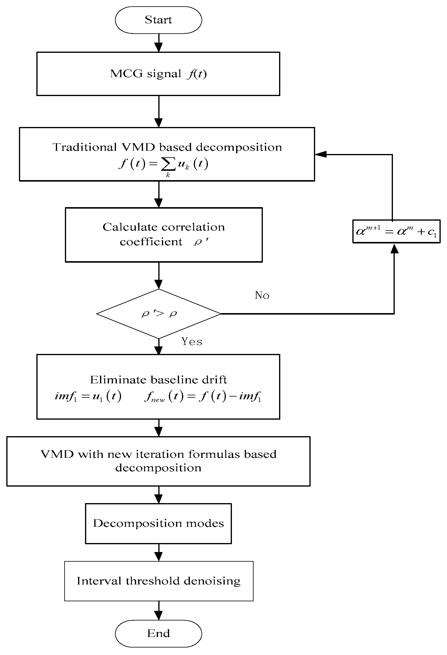
Summarizing this denoising process as follows: First, the MCG signal with noise is decomposed into corresponding IMFs by improved VMD. The first order IMF, including the baseline drift noise, is eliminated. Second, the interval thresholding is performed on the rest IMFs. Clearly, the higher the order, the greater the frequency of the IMF. The detailed procedures are as follows:
- Acquire the MCG signal with noise and initialize the number of modes k, the default of the penalty factor is 2000, the default of the bandwidth is 0.
- Determine the value of penalty factor by performing the improved VMD method based on the correlation coefficient and obtain the first IMF.
- Eliminate the first IMF that contains baseline drift noise. Decompose the rest signal with the final update formulas and obtain several IMFs.
- Perform the interval thresholding operation on the IMFs obtained from step 3.
- Add all the processed IMFs together and refactor the MCG signal.
In Figure 1 we show the flow chart of the improved VMD algorithm:
4. Results and Discussion
Three different types of noise have been added to the MCG signal, in order to investigate the effectiveness of denoising by an improved VMD and the interval thresholding method. The types of noise include a low frequency (0.3 Hz) sinusoidal signal for simulating the baseline drift, 50 Hz sinusoidal signal for simulating the interference at power line frequency, and high frequency random noise. In Figure 2, we compare the waveforms of an original simulation signal and a mixed signal. It is clearly seen that background noise affects signal analysis. It is very significant in the process of measuring MCG signals to detect heart disease.
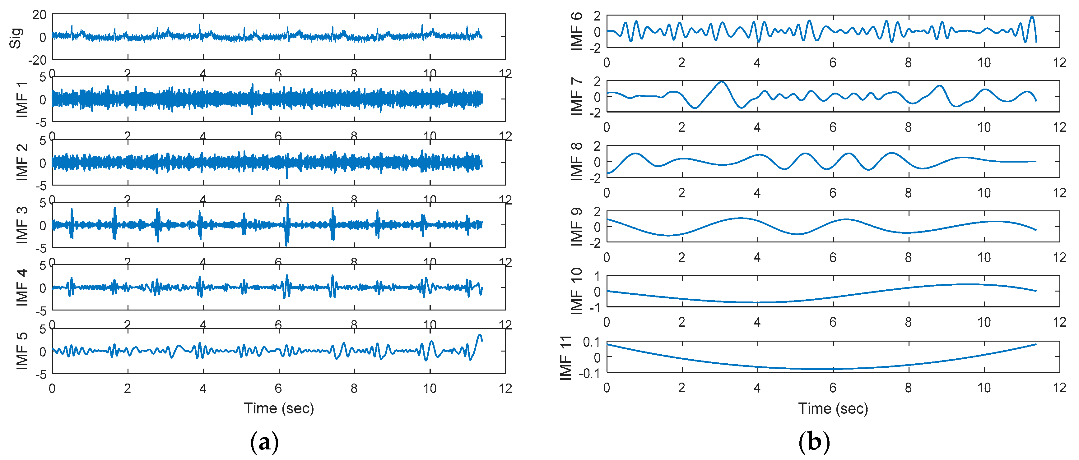
The signal is denoised by different algorithms. In Figure 3a,b, we show the signal decomposition results obtained by the EEMD method. In Figure 3, according to the length of the data, the MCG signal is decomposed into ten IMFs, and the frequency of IMFs reduces as the order increases. In general, the low frequency smooth variation of the baseline is expected to be contained in the residue of the higher order IMFs. However, we cannot determine the low-frequency component that contains baseline drift noise. It is evident that we can extract signal characteristics from IMF2 to IMF6. Unfortunately, other IMFs may also contain useful signal components that are invisible to the human eye. Given this, we apply thresholds only to a few low order IMFs that contain contributions from the high frequency noise components, then exclude a few high order IMFs that contain the low frequency contents with a view, to ensure that the low frequency contents of the MCG signal are not affected or distorted by thresholding.
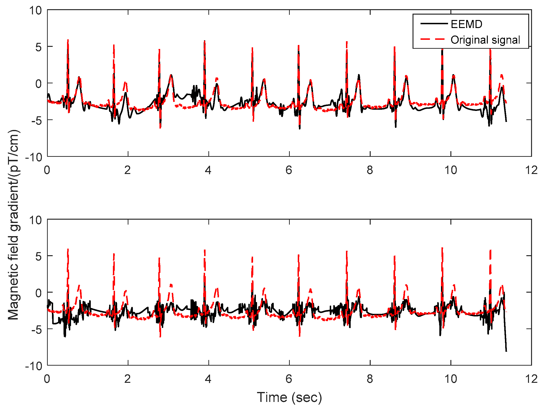
In Figure 4, we compare the original signal with the reconstructed signals obtained from EEMD based denoising methods using soft and hard thresholding. The results show that the hard threshold processing can reconstruct the QRS peak waves, but there are obvious errors in the reconstruction of other signal parts. The signal obtained by soft thresholding processing has errors compared with the original signal, especially the QRS peaks. It is seen from Figure 4 that EEMD algorithm is difficult to distinguish noise components from signal components. And the number of low frequency IMFs is too many to result in waveform distortion after performing thresholding operation. It may also be noted that, hard-IT (hard thresholding subsequently interval thresholding) is adopted for EEMD based denoising of the experimental data. At the same time, we can see that the signal waveform is not smooth and slightly distorted.
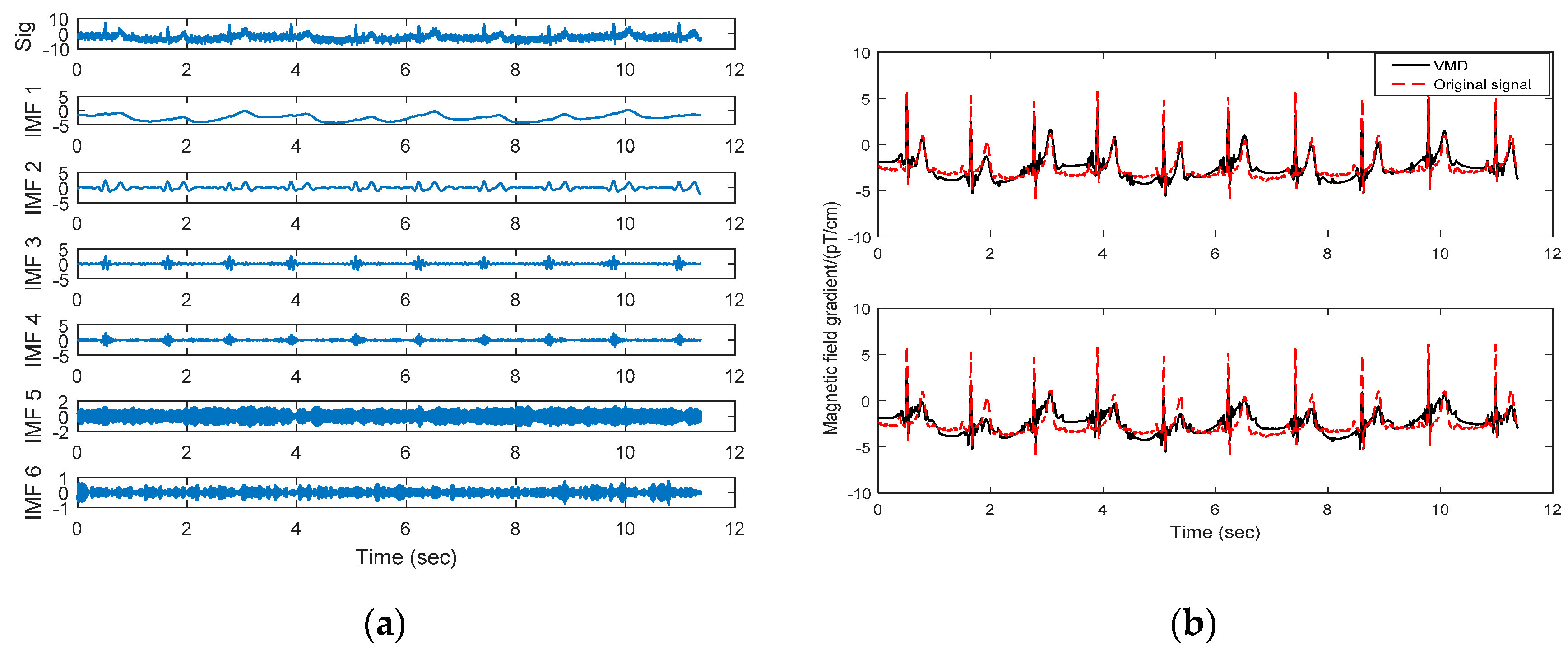
Based on the bandwidth of the measurement signal and multiple tests, the number of modes decomposed by VMD is assigned to 6. The original algorithm proposer studied some of the convergence characteristics of the VMD algorithm and its sensitivity to the initial conditions, then got relatively suitable initialization parameters. The initial value of quadratic penalty is assigned to 2000, and the default of the bandwidth is 0. With this method, the MCG signal is divided into several frequency bands centering on respective center frequency, which benefits subsequent operation. As shown in Figure 5a, the MCG signal is divided into six IMFs. The baseline drift noise is found in IMF1. In Figure 5b, we compare the original signal with the reconstructed signals obtained from VMD methods with soft and hard thresholding. The results show that the baseline of the reconstructed signal is not uniform with the original signal. To make matters worse, there is serious distortion in the reconstructed signal from the soft thresholding processing. It is obvious that the algorithm cannot effectively remove baseline drift noise. The decomposition process of the algorithm lacks of adaptability. Improper decomposition results can easily lead to waveform distortion after threshold processing.
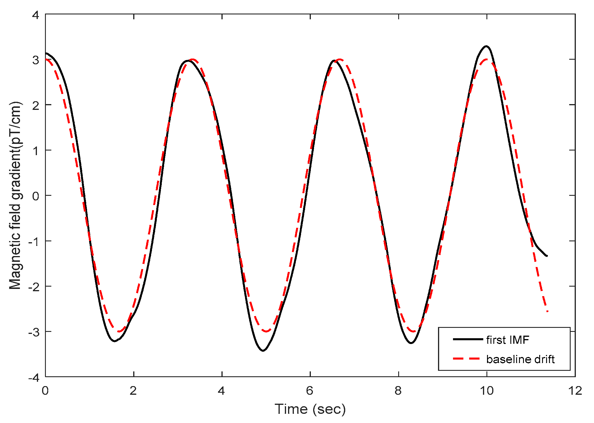
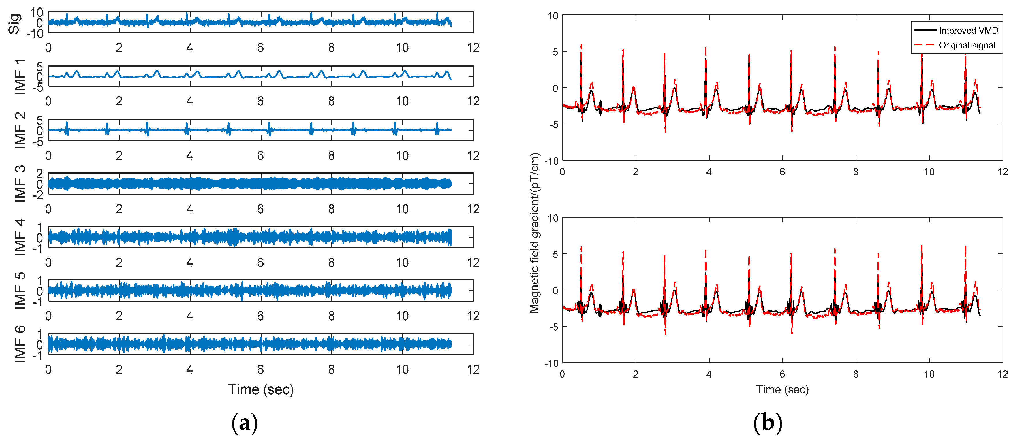
To get a better result, we use the proposed method to decompose the signal. According to many experiments, we choose the parameter value with better effect as the next simulation initial values. The threshold value of correlation coefficient is assigned as 0.95. The value of the scaling factor is the range 1500 and 2000. The value of can be set according to the detailed data features and is assigned as 3.5. As Figure 6 shown, the baseline noise is extracted. After removing the noise, the signal is divided into six modes adaptively. According to iterative formulas for multiple iterations, the penalty factors for six components are [1790, 987, 956, 218, 223, 208]. The decomposition results are shown in Figure 7a and the denoising results are shown in Figure 7b.
The range of the value of the penalty factors can support the adaptive decomposition result. From this result, it can be seen that the low-frequency IMF’s penalty factors are large, and the penalty factor increases approximately with the increasing of the center frequency, achieving the purpose of the meticulous decomposition of low-frequency signal component. In addition, we can obtain a set of different penalty factors by adjusting the size of to adjust the decomposition result. By comparing the reconstructed signal with the original signal, we can find that the fitting degree between the reconstructed signal and the original signal is good, and all three kinds of noise in the signal are effectively removed. It may also be noted that, signal to noise ratio improvement is much better of the hard interval thresholding (IT) method compared to the soft interval thresholding.
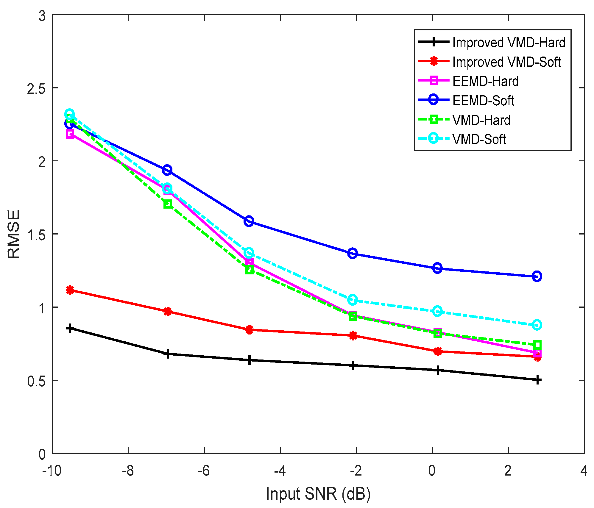
In order to better compare the performance of the algorithms, we use the root-mean-square error (the square root of the mean of the sum of squared residuals, RMSE) to characterize the fitting degree of the reconstructed signal and the original signal. In Figure 8, we compare the root-mean-square deviation (RMSE) of the three methods with the input signal-to-noise ratio (SNR). In the case of low input SNR, the RMSE of the improved VMD method is significantly less than the other two methods, and the method has better denoising performance even with the low input SNR.
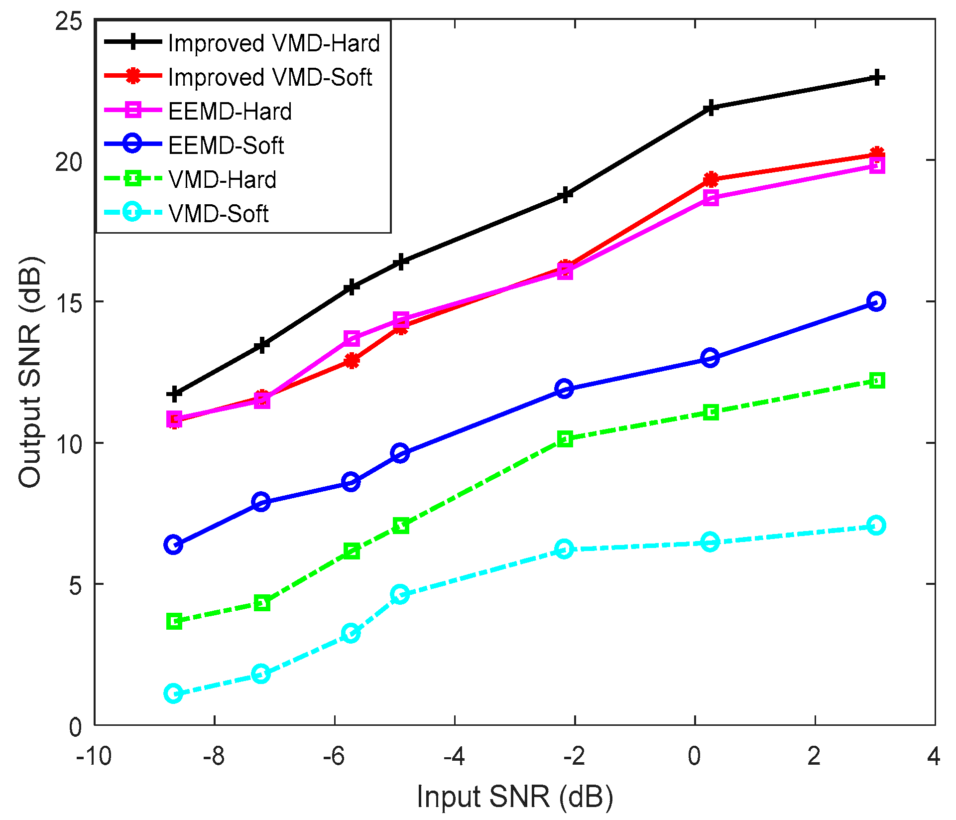
In Figure 9, we compare the performance of the original VMD method, the improved VMD method, and the EEMD methods, using soft and hard thresholding in each case. For computing SNR, the logarithmic ratio of variance of a signal (from the beginning of P-wave to the end of T-wave for one cardiac cycle) to the variance of noise (from the end of T-wave to the beginning of P-wave, i.e., in the TP interval) has been taken. The reduction in the SNR for the soft thresholding method is due to the reduction of signal components of the lower frequency IMFs. Hereafter, hard-IT (hard thresholding is subsequently applied to the interval thresholds) is appropriate for both EEMD and VMD based denoising of the experimental data. It is seen from Figure 9 that the improved VMD method is capable of achieving better SNR when compared with EEMD and VMD methods.
From the above simulation results, we can see that the proposed algorithms have better denoising performance compared with EEMD and VMD methods. It should be noted, however, that the waveform is still distorted, even by the proposed method; this is a crucial detail in electrocardiographic-like signals. One encouraging factor, is that results of medical research have shown that the QRS spikes and S-T waves contain information on the main electrical function parameters of the heart. The MCG signal is filtered by the algorithm proposed in this paper, in order to obtain QRS spikes and S-T waves that approximate the original signal. Although there are slight disturbances in the QRS spikes and S-T waves obtained by filtering, it does not affect the calculation of heart related parameters! Measurements of magnetic field energy and current density remain accurate). In the case of the low input signal-to-noise ratio used in this paper, the SNR improvement of the proposed algorithm can be up to 20 dB. The algorithm filtering results can support feature extraction of MCG and detection of heart disease.
Despite these positive results, the MCG signals measured in a clinical non-magnetic shielding environment would still contain a large amount of background noise, which would still cause the waveform, denoised by the improved VMD method proposed in this paper, to produce severe distortion. In order to solve this problem, we need to study the spatial filtering technology in order to further denoise the MCG signal, in efforts to achieve the purpose of joint filtering in the time domain, frequency domain, and space domain.
5. Conclusions
The proposed method in this paper overcomes the unadaptable quadratic penalty problem of VMD, which improves the availability and precision of denoising of the MCG signal. This method adaptively adjusts the bandwidth of modes by repeatedly executing the VMD method with different quadratic penalties. The low-frequency noise is eliminated, according to the correlation coefficient for baseline drift noise, and the first mode. The new update formulas are used to decompose residual signals adaptively. Then, threshold processing is performed on each IMF to eliminate other noise. The simulation experiments show the superiority of the improved VMD in denoising performance of the MCG signal. The acceleration of the proposed method, and the suitable signal preprocessing methods, should be considered in future research and applications.
Author Contributions
Conceptualization, Y.L. and Q.G.; Methodology, C.H.; Software, C.H.; Validation, Y.L. and Q.G.; Writing—original draft, C.H.; Writing—review & editing, Y.L. and C.H.
Funding
This work is supported partially by the National Key Research and Development Program of China (2016YFC0101700), by National Natural Science Foundation of China 61301201 and 61371175, Heilongjiang Postdoctoral Research Foundation LBH-Q14039.
Acknowledgments
The authors are grateful to the anonymous referees for their valuable comments and suggestions that improved this paper.
Conflicts of Interest
The authors declare no conflicts of interest.
References
- Mäkijärvi, M.; Montonen, J.; Toivonen, L. Identification of patients with ventricular tachycardia after myocardial infarction by high-resolution magnetocardiography and electrocardiography. J. Electrocardiol. 1993, 26, 117–124. [Google Scholar] [CrossRef]
- Shanehsazzadeh, F.; Fardmanesh, M. Low Noise Active Shield for SQUID-Based Magnetocardiography Systems. IEEE Trans. Appl. Supercond. 2017, 99, 1–5. [Google Scholar] [CrossRef]
- Farré, J.; Shenasa, M. Medical Education in Electrocardiography. J. Electrocardiol. 2017, 50, 400–401. [Google Scholar] [CrossRef] [PubMed]
- Fenici, R.; Brisinda, D. Magnetocardiography provides non-invasive three-dimensional electroanatomical imaging of cardiac electrophysiology. Anatol. J. Cardiol. 2006, 22, 595. [Google Scholar] [CrossRef] [PubMed]
- Ha, T.; Kim, K.; Lim, S. Three-Dimensional Reconstruction of a Cardiac Outline by Magnetocardiography. IEEE Trans. Biomed. Eng. 2015, 62, 60–69. [Google Scholar] [CrossRef] [PubMed]
- Mariyappa, N.; Parasakthi, C.; Sengottuvel, S. Dipole location using SQUID based measurements: Application to magnetocardiography. Phys. C Supercond. 2012, 477, 15–19. [Google Scholar] [CrossRef]
- Tiporlini, V.; Alameh, K. Optical Magnetometer Employing Adaptive Noise Cancellation for Unshielded Magnetocardiography. Univ. J. Biomed. Eng. 2013, 1, 16–21. [Google Scholar] [CrossRef]
- Kim, K.; Lee, Y.H.; Kwon, H. Averaging algorithm based on data statistics in magnetocardiography. Neurol. Clin. Neurophysiol. 2004, 2004, 42. [Google Scholar] [PubMed]
- Dang-Ting, L.; Ye, T.; Yu-Feng, R.; Hong-Wei, Y.; Li-Hua, Z.; Qian-Sheng, Y.; Geng-Hua, C. A novel filter scheme of data processing for SQUID-based Magnetocardiogram. Chin. Phys. Lett. 2008, 25, 2714–2717. [Google Scholar] [CrossRef]
- Tiporlini, V.; Nguyen, N.; Alameh, K. Adaptive noise canceller for magnetocardiography. In Proceedings of the High Capacity Optical Networks and Enabling Technologies, Riyadh, Saudi Arabia, 19–21 December 2011; pp. 359–363. [Google Scholar]
- Dong, Y.; Shi, H.; Luo, J. Application of Wavelet Transform in MCG-signal Denoising. Mod. Appl. Sci. 2010, 4, 20. [Google Scholar] [CrossRef]
- Huang, N.E.; Shen, Z.; Long, S.R.; Wu, M.C.; Shih, H.H.; Zheng, Q.; Yen, N.C.; Tung, C.C.; Liu, H.H. The empirical mode decomposition and the Hilbert spectrum for nonlinear and non-stationary time series analysis. Proc. R. Soc. Lond. A 1998, 454, 903–995. [Google Scholar] [CrossRef]
- Attoh-Okine, N.; Barner, K.; Bentil, D.; Zhang, R. Editorial: The empirical mode decomposition and the hilbert-huang transform. EURASIP J. Adv. Signal Process. 2008. [Google Scholar] [CrossRef]
- Wu, Z.; Huang, N.E. Ensemble empirical mode decomposition method: A noise-assisted data analysis method. Adv. Adapt. Data Anal. 2009, 1, 1–41. [Google Scholar] [CrossRef]
- Tong, W.; Zhang, M.; Yu, Q. Comparing the applications of EMD and EEMD on time–frequency analysis of seismic signal. J. Appl. Geoph. 2012, 83, 29–34. [Google Scholar]
- Mariyappa, N.; Sengottuvel, S.; Parasakthi, C. Baseline drift removal and denoising of MCG data using EEMD: Role of noise amplitude and the thresholding effect. Med. Eng. Phys. 2014, 36, 1266–1276. [Google Scholar] [CrossRef] [PubMed]
- Mariyappa, N.; Sengottuvel, S.; Patel, R. Denoising of multichannel MCG data by the combination of EEMD and ICA and its effect on the pseudo current density maps. Biomed. Signal Process. Control. 2015, 18, 204–213. [Google Scholar] [CrossRef]
- Smruthy, A.; Suchetha, M. Real-Time Classification of Healthy and Apnea Subjects Using ECG Signals With Variational Mode Decomposition. IEEE Sens. J. 2017, 17, 3092–3099. [Google Scholar] [CrossRef]
- Dragomiretskiy, K.; Zosso, D. Variational Mode Decomposition. IEEE Trans. Signal Process. 2014, 62, 531–544. [Google Scholar] [CrossRef]
- Sun, Z.G.; Lei, Y.; Wang, J. An ECG signal analysis and prediction method combined with VMD and neural network. In Proceedings of the IEEE International Conference on Electronics Information and Emergency Communication, Macau, China, 21–23 July 2017; pp. 199–202. [Google Scholar]
- Maji, U.; Pal, S. Empirical mode decomposition vs. variational mode decomposition on ECG signal processing: A comparative study. In Proceedings of the International Conference on Advances in Computing, Communications and Informatics, Jaipur, India, 21–24 September 2016; pp. 1129–1134. [Google Scholar]
- Mert, A. ECG signal analysis based on variational mode decomposition and bandwidth property. In Proceedings of the IEEE Signal Processing and Communication Application Conference, Zonguldak, Turkey, 16–19 May 2016; pp. 1205–1208. [Google Scholar]
- Viswanath, A.; Jose, K.J.; Krishnan, N. Spike Detection of Disturbed Power Signal Using VMD ☆. Procedia Comput. Sci. 2015, 46, 1087–1094. [Google Scholar] [CrossRef]
- Kopsinis, Y.; Mclaughlin, S. Development of EMD-Based Denoising Methods Inspired by Wavelet Thresholding. IEEE Trans. Signal Process. 2009, 57, 1351–1362. [Google Scholar] [CrossRef]
- Daubechies, I.; Lu, J.; Wu, H.T. Synchrosqueezed wavelet transforms: An empirical mode decomposition-like tool. Appl. Comput. Harmonic Anal. 2011, 30, 243–261. [Google Scholar] [CrossRef]
- Gilles, J. Empirical Wavelet Transform. IEEE Trans. Signal Process. 2013, 61, 3999–4010. [Google Scholar] [CrossRef]
- Unser, M.; Sage, D.; Van, D.V.D. Multiresolution monogenic signal analysis using the Riesz-Laplace wavelet transform. IEEE Trans. Image Process. 2009, 18, 2402–2418. [Google Scholar] [CrossRef] [PubMed]
- Bertsekas, D.P. Multiplier methods: A survey. Automatica 1976, 12, 133–145. [Google Scholar] [CrossRef] [Green Version]
- Hestenes, M.R. Multiplier and gradient methods. J. Optim. Theory Appl. 1969, 4, 303–320. [Google Scholar] [CrossRef]
- Rockafellar, R.T. A dual approach to solving nonlinear programming problems by unconstrained optimization. Math. Program. 1973, 5, 354–373. [Google Scholar] [CrossRef] [Green Version]
- Boley, D. Local Linear Convergence of the Alternating Direction Method of Multipliers on Quadratic or Linear Programs. Siam J. Optim. 2013, 23, 2183–2207. [Google Scholar] [CrossRef] [Green Version]
Figure 1.
The flow chart of the improved Variational Mode Decomposition (VMD) algorithm.

Figure 2.
A comparison of the approximately pure magnetocardiography (MCG) signal with the noisy signal; waveform characteristics can be clearly seen in (a); (b) shows the signal waveform with three kinds of noise. The signal is drowned in the noise under high noise circumstances.
Figure 2.
A comparison of the approximately pure magnetocardiography (MCG) signal with the noisy signal; waveform characteristics can be clearly seen in (a); (b) shows the signal waveform with three kinds of noise. The signal is drowned in the noise under high noise circumstances.

Figure 3.
The noisy signal and the intrinsic mode functions (IMFs) obtained by Ensemble Empirical Mode Decompositioning (EEMD) are shown in (a,b).
Figure 3.
The noisy signal and the intrinsic mode functions (IMFs) obtained by Ensemble Empirical Mode Decompositioning (EEMD) are shown in (a,b).

Figure 4.
A comparison of the original signal (dotted line) with the reconstructed signals (solid line) obtained from EEMD based denoising methods with soft and hard thresholding. The panel above is the result of hard thresholding processing and the following panel is the result of soft thresholding processing.

Figure 5.
The noisy signal and the IMFs obtained from VMD are shown in (a). A comparison of the original signal (dotted line) with the reconstructed signals (solid line) obtained from VMD based denoising methods with soft and hard thresholding is shown in (b). The panel above is the result of hard thresholding processing and the following panel is the result of soft thresholding processing.

Figure 6.
The first IMF obtained from the improved VMD method (solid line) and baseline drift noise (dotted line). It is seen that the solid line and the dotted line basically coincide. This method can effectively remove baseline drift noise.
Figure 6.
The first IMF obtained from the improved VMD method (solid line) and baseline drift noise (dotted line). It is seen that the solid line and the dotted line basically coincide. This method can effectively remove baseline drift noise.

Figure 7.
(a) The noisy signal and the IMFs obtained from the improved VMD method; (b) A comparison of the original signal (dotted line) with the reconstructed signals (solid line) obtained from the improved VMD method with soft and hard thresholding for interval thresholding. The panel above is the result of hard thresholding processing and the following panel is the result of soft thresholding processing.

Figure 8.
The root-mean-square deviation (RMSE) of the EEMD, the VMD, and the improved VMD methods are revealed, for both soft and hard thresholding of interval thresholding. The improved VMD method outperforms other methods.
Figure 8.
The root-mean-square deviation (RMSE) of the EEMD, the VMD, and the improved VMD methods are revealed, for both soft and hard thresholding of interval thresholding. The improved VMD method outperforms other methods.

Figure 9.
The variation of the output signal-to-noise ratio (SNR) by EEMD, VMD and the improved VMD methods with soft and hard thresholds for interval thresholding. The improved VMD method outperforms other methods.
Figure 9.
The variation of the output signal-to-noise ratio (SNR) by EEMD, VMD and the improved VMD methods with soft and hard thresholds for interval thresholding. The improved VMD method outperforms other methods.

© 2018 by the authors. Licensee MDPI, Basel, Switzerland. This article is an open access article distributed under the terms and conditions of the Creative Commons Attribution (CC BY) license (http://creativecommons.org/licenses/by/4.0/).
Share and Cite
MDPI and ACS Style
Liao, Y.; He, C.; Guo, Q. Denoising of Magnetocardiography Based on Improved Variational Mode Decomposition and Interval Thresholding Method. Symmetry 2018, 10, 269. https://doi.org/10.3390/sym10070269
AMA Style
Liao Y, He C, Guo Q. Denoising of Magnetocardiography Based on Improved Variational Mode Decomposition and Interval Thresholding Method. Symmetry. 2018; 10(7):269. https://doi.org/10.3390/sym10070269
Chicago/Turabian StyleLiao, Yanping, Congcong He, and Qiang Guo. 2018. "Denoising of Magnetocardiography Based on Improved Variational Mode Decomposition and Interval Thresholding Method" Symmetry 10, no. 7: 269. https://doi.org/10.3390/sym10070269
Note that from the first issue of 2016, this journal uses article numbers instead of page numbers. See further details here.