Article

On the Symmetry of the Bone Structure Density over the Nasopalatine Foramen via Accurate Fractal Dimension Analysis

by
Michael M. Bornstein
1,
Manuel Fernández-Martínez
2,
Juan L. G. Guirao
3,*,
Francisco J. Gómez-García
4,
Yolanda Guerrero-Sánchez
4 and
Pía López-Jornet
4
1
Department of Applied Oral Sciences of the Faculty of Dentistry, University of Hong Kong, Hong Kong, China
2
University Center of Defence at the Spanish Air Force Academy, MDE-UPCT, 30720 Santiago de la Ribera, Murcia, Spain
3
Departamento de Matemática Aplicada y Estadística, Universidad Politécnica de Cartagena, Hospital de Marina, 30203 Cartagena, Región de Murcia, Spain
4
Department of Dermatology, Stomatology, Radiology and Physical Medicine, Morales Meseguer General Universitary Hospital, Avda. Marqués de los Vélez, 30008 Murcia, Spain
*
Author to whom correspondence should be addressed.
Symmetry 2019, 11(2), 202; https://doi.org/10.3390/sym11020202
Submission received: 17 December 2018 / Revised: 1 February 2019 / Accepted: 3 February 2019 / Published: 11 February 2019
(This article belongs to the Special Issue New Trends in Dynamics)

Abstract

:
The objective of the present paper is to describe all the anatomical considerations surrounding the nasopalatine foramen by relating them to the study of bone structure density via an accurate fractal dimension analysis in that area. We consecutively selected a sample of 130 patients, all of them with cone beam computed tomography (CBCT) images performed for treatment needs. We chose a specific window (ROI), which coincides with an axial cut at the level of the anterior nasal spine. Different anthropometric measurements were analyzed and a novel fractal dimension analysis was performed. Our sample consisted of 130 patients and was divided into two groups: group one (consisting of 65 subjects without loss of teeth) and group two (consisting of 65 patients with the absence of some teeth). In the sample, 52.31% were women (68 people). Mann–Whitney tests were applied to obtain the statistical results. The mean age of the patients in that sample was 53.67 years with a standard deviation of 8.20 years. We conclude that fractal dimension, a mathematical invariant, behaves symmetrically for binary images from the CBCT scanners of each subject of our sample of study. We also conclude that there were no significant differences between all the anthropometric measures used neither in the subjects themselves nor in the different groups. Therefore, some patterns of symmetry were appreciated at a complete range of levels.

1. Introduction

Embryologically, the formation (histogenesis) and mineralisation (ossification) of hard facial tissues takes place after that of the soft tissues, at the end of embryonic period (10–12 weeks). There are two types of ossification. On the one hand, intramembranous, made from mesenchyme, which will become osteoid ossification centers, and will be arranged by forming a 3D network of trabeculae. The other type is an endochondral or cartilaginous mold, in which a cast of hyaline cartilage will be replaced by bone tissue. The type of ossification will depend on the future function of the bone. In growth areas exposed to stress, the mechanism of ossification is intramembranous. The ossification is endochondral wherever there is pressure, since the cartilage is rigid and flexible, properly supporting this type of loads. Intramembranous ossification predominates in face bones or viscerocranium. The ossification of maxillary bone commences at the end of the sixth week of intrauterine life and takes place from two points, one of them located in the anterior (premaxillary), and the another one in the posterior (postmaxillary) area. The trabeculae formed from the premaxillary ossification center are rapidly directed in three directions: (1) upward, to form the anterior wall of the descending process; (2) forward, towards the anterior nasal spine; and (3) downward, to form the alveolar processes of upper incisors. Both cranial and facial growths are performed in the three dimensions of space. Usually, it is harmonic and proportional though not uniform. That growth is produced by the combination of four different biological phenomena, namely, (1) replacement of cartilage by bone; (2) growth at suture level; (3) peripheral bone affectation associated with internal resorption; and (4) dental rash [1]. From an anatomic viewpoint, maxillary bone is part of mass or facial bone complex, being its functional center. The external configuration of upper jaw is quite irregular. However, a quadrilateral shape may be recognized so both external and internal faces are distinguished as well as four edges. Maxillary bone is even and fused in the midline by intermaxillary suture so it constitutes the center of upper facial mass. As such, it is part of buccal cavity, bony palate, orbital, nasal, pterygopalatine, and zygomatic pits. We would like to point out that maxillary bone consists of:
  • Body: it is most of the bone, pyramidal, is part of orbit, nasal cavity, infratemporal fossa, and the middle third of the face. It presents, in its anterior region, both the anterior nasal spine and the nasal notch.
  • Frontal apophysis, which is articulated with nasal, frontal, ethmoid, and lacrimal bones.
  • Zygomatic apophysis, that is articulated medially with the maxillary process of zygomatic bone.
  • Palatine process, extending medially by forming the greatest part of hard palate, articulating in the middle line with the contralateral maxilla one, and later with palatal bone, and
  • Alveolar process, which supports the upper teeth. The convex region that covers canine by vestibular is the canine eminence. There is a concavity mesial to this, i.e., the incisive fossa. Also, the canine fossa is a concavity which is distal to the canine one. The most posterior region of the alveolar process is the tuberosity of the maxilla [2].
Topographically, there are three zones, namely,
  • Anterior zone, which covers from the intermaxillary suture to the canine eminence.
  • Middle zone: canine eminence and zygomatic-alveolar or infratemporal crest, and
  • Posterior zone: distal to zygomatic-alveolar crest.
The anterior maxilla, also called as the premaxilla area, contains a key anatomical structure, the anterior palatal, incisor, or nasopalatine canal (NPC in the sequel). NPC is located immediately below the incisive papilla. Both anterior palatine ducts open into the incisive fossa of the osseous palate, and possibly pass through the junction line of the incisor (premaxillary) bone with the maxilla. It constitutes the primitive communication between the mouth and the nose. NPC was first described in a general way by Stenson in 1683. It is located in the midline of the palate, posterior to the central incisors, and below the interincisal papilla. It is projected vertically in the premaxillary region and consists of two extremes: one towards the nasal floor with two openings being directed towards each side of the septum, known as foramines or Stenson holes; the second end corresponds to the opening towards the oral cavity, called incisor hole, whose diameter is equal to 3.62 mm. That anatomical structure houses both the nasopalatine nerve and the nasopalatine artery, which originates from the sphenopalatine artery (terminal branch of the internal maxillary), both going to innervate and simultaneously irrigating the nasal floor mucosa and the anterior palatal mucosa. NPC is also composed of fibrous connective tissue, fatty tissue, and some minor salivary glands [3]. The balance, symmetry, and harmony between facial structures are fundamental elements in the attainment of facial beauty, since it plays a fundamental role in the psychosocial development of the individual. In this sense, due to the close relationship of teeth with the formation and preservation of alveolar processes, the loss of these causes an irreversible process of reduction of bone volume, both horizontally and vertically, which is greater in the maxilla, higher in the jaw, and vestibular in the palatine, with serious clinical, functional, and aesthetic implications [4]. The rhythm of that bone loss depends on several factors, such as the existence of more teeth in the arch, maneuvers performed for exodontia, and the presence of previous infectious or cystic pathology, as well as the complication of healing by alveolitis. Patients with a long period of partial or total edentulism suffer severe atrophy of the jaws, with great asymmetry of dental arches. As a consequence, the retention and stability of partial or complete removable prostheses is negatively affected [5]. Currently, in developed countries, dental implants are considered the best option to replace lost teeth with others (removable prosthesis or bridge). However, in case of bone deficiency, the placement of implants may be quite complicated, especially in the maxilla, where the bone loss may be so pronounced that the floor of the maxillary sinus is practically in contact with the palatal fibromucosa. In such cases, it becomes necessary to perform maneuvers of bone volume increase to allow the placement of implants with greater length and diameter, and in a more favorable position, thus improving the results in the medium and long term [6]. These advanced oral surgery techniques require a thorough morphological study of the area to be treated, for which 3D radiology is essential. When no distortion is found, that type of technique allows better planning of implant treatments according to the receptor site. In this way, the cone beam computed tomography (CBCT) allows clinicians to carry out a variety of analyzes to know the characteristics of bone structures, such as bone quality, or to inspect the topography and thickness of cortical bones. Bone volume can be examined essentially to predict vascularity for bone maturation and preservation. Bone defect detections are crucial to decide on a graft procedure. The use of CBCT specialized in dentomaxillofacial area has been a step forward compared to conventional CT for its greater precision, lower cost, radiation, accessibility, and short duration of the scanner [7]. The most relevant anatomical formation of the anterior region of the maxilla is the NPC. In the scientific literature, surgical difficulties and anatomical limitations during implant surgery have been described in relation with the location of that structure. In the study conducted by Bornstein et al. [8] to evaluate the different anatomical variations of NPC, they found a single channel that was identified in 45 cases, two parallel channels separated in 15 cases, and variations of the “Y” type, that were observed in 40 cases. The dimensions of the NPC revealed an average diameter of the nasal openings of 3.49 mm, and a broad incisive foramen with a diameter equal to 4.45 mm. The average length of the NPC was found to be equal to 10.99 mm. The dimensions of the buccal bone plate showed an increasing width from the crest to the apical measurements. Liang et al. [9] in 2009, conducted a study to determine the anatomical variability of NPC as well as its characteristics, both anatomical and histological. The diameter of the canal was found to be enlarged with age and in edentulous patients. In 2018, Hakbilen et al. [10], analyzed three-dimensionally (by CBCT) the anatomical dimensions of NPC of 619 individuals aged from 17 to 86 years, and correlated them with age, gender, and edentulism status. They found large morphological differences among individuals. In particular, 26.17 % of them had a conical shape, 24.71 % were hourglass, 16.80 % cylindrical, 15.83 % funnel, 11.14 % banana, and 5.33 % of the channels were branched. Men and women showed significant differences in regard to the length of the channels, as well as in the thickness of the vestibular cortices in the sagittal sections. Age and edentulism also affected the length of the NPC and the thickness of the vestibular cortex.
The knowledge about the establishment of theories that may clarify the etiopathogenesis of the development of the nasopalatine region and NPC in humans becomes necessary to understand the morphology of such a region and the morbidity that takes place therein, being the tomography a great help for that purpose. Related to all these types of studies that have been conducted there has never been a parallel study of the bone density analysis. The studies we have reviewed always use the same technique to deal with fractal dimension calculations, namely, the box-counting technique ([8,9]). As we have explained previously ([10,11]), our technique consists of a much more precise algorithm that throws reliable results, much closer to reality than the others. In summary, the objective of this work is to carry out an exhaustive analysis of the area surrounding the nasopalatine foramen, helping us with new mathematical techniques with the idea of detect generic symmetry patterns to provide some empirical evidence that bony trabeculate resembles in its structure a fractal, and therefore, possesses a fractal dimension whose real value can be accurately approximated by our procedure. As such, the main research question in this study is as follows: Are there patterns of symmetry on bone structure density over nasopalatine foramen?

2. Materials and Methods

This is a cross-sectional and observational clinical study for which we selected a sample of 153 patients consecutively from the University dental clinic of Murcia (Spain). The study was approved by the Bioethics Committee of the University of Murcia. All individuals gave their informed consent in writing before participating. The following inclusion criteria were applied; patients in health conditions both systemic and dental, not pregnant, images that do not contain artefacts. A total amount of 130 patients that met all the criteria described above (five were discarded because they were submitted to treatments with bisphosphonates as well as 18 other subjects, since their images presented artefacts or were not considered with enough quality to be able to apply our fractal dimension procedure). All CBCTs were performed using the same Planmeca® equipment, Planmeca ProMax 3D Max (Planmeca Oy, Helsinki, Finland) calibrated according to technical considerations. X-rays were obtained with the patient in the same position (prone position). The beam emission parameters were kV = 96 , mA = 8 , exposure time of 12 s ( 11.94 s) with an image size of 501 × 501 × 466 voxels (each voxel being equivalent to 200 μ m). The evaluation software used was the Romexis 2.5.1® program (Planmeca Oy, Helsinki, Finland), which allowed observing the image in a multiple window where the axial, coronal and sagittal planes can be visualized in 0.2 mm intervals, in addition to a 3D vision. As indicated above, the sample was divided into three groups. We proceed to select a specific ROI that was obtained in the axial plane at the height of the nasal spine, visualising the nasopalatine foramen and the canine mamelons on both sides, see Figure 1.
We proceed to make the following measurements; distance anterior wall nasopalatine hole to anterior nasal spine (DCV), distance back wall foramen (NF) to border palate bone (DCP), distance right side wall NF to right canine mamelon (DVD), distance left lateral wall NF to left canine mamelon (DVI), area of the NF and other values provided by the software itself: W, H, mean, and standard deviation. All measurements were made by a single examiner duly trained for the purpose. The measurements were repeated by the examiner one month after performing the first ones and if there was a discrepancy in any measurement, the average of both is obtained and the kappa index was used. Once all the results were obtained, a database was created, and the necessary Mathematica® code was written to perform all the statistical analyses.

3. Results and Discussion

3.1. Description of the Sample

In this section, we shall describe the sample of patients that took part in our study. 130 subjects were involved with 52.31 % (68 people) being women. Each patient was assigned to one of the two following groups. Group one consisted of 65 patients, all of them without loss of teeth, and 65 subjects were assigned to group two (with the absence of some dental pieces). A first descriptive analysis was carried out with the aim to characterize our sample of patients. As such, for each patient in our study, the following attributes were considered.
  • Age: it was found a mean age equal to 53.67 years with a standard deviation of 8.20 years.
  • DCV: a mean of 7.54 and a standard deviation equal to 1.53 were found.
  • DCP: with a mean of 3.99 and a standard deviation equal to 1.65 .
  • DVD: a mean of 12.95 and a standard deviation of 1.75 were obtained.
  • DVI: with a mean of 12.98 and a standard deviation equal to 1.34 .
  • Area: a mean of 5.63 and a standard deviation equal to 2.18 were found.
  • W: a mean equal to 2.96 and a standard deviation of 0.71 were found.
  • H: with a mean equal to 2.23 and a standard deviation of 0.59 .
  • Mean: a mean equal to 158.66 and a standard deviation of 120.83 was obtained.
  • DIM: a mean fractal dimension of 1.69 and a standard deviation equal to 0.09 were found.
Table 1 summarizes the sample description by attributes.

3.2. Sample Description by Sex

Next, we shall describe in detail our sample of patients by sex groups.

3.2.1. Female Population

It contained 68 subjects ( 52.31 % of the whole sample) of which 34 people were assigned to group one and 34 people were assigned to group two. In regard to the attributes explored for each female patient in the present study, the results we obtained are as follows.
  • Age: a mean age of 54.62 years with a standard deviation equal to 8.99 years was found.
  • DCV: a mean equal to 7.29 and a standard deviation of 1.63 were obtained.
  • DCP: with a mean equal to 4.05 and a standard deviation equal to 1.69 .
  • DVD: a mean of 12.82 and a standard deviation equal to 1.62 were found.
  • DVI: it was found a mean equal to 12.38 with a standard deviation of 1.62 .
  • Area: with a mean equal to 5.33 and a standard deviation equal to 1.98 .
  • W: a mean equal to 3.03 and a standard deviation of 0.72 were found.
  • H: a mean of 2.26 and a standard deviation equal to 0.44 were found.
  • Mean: a mean of 142.65 and a standard deviation of 107.52 were obtained.
  • DIM: a mean fractal dimension of 1.68 and a standard deviation equal to 0.13 were found.

3.2.2. Male Population

It contained 62 people ( 47.69 % of the whole sample) in our study. Of them, 31 people were assigned to group one and 31 were assigned to group two. Similarly to our female population, some descriptive statistics regarding the attributes of the male one were calculated. The results are provided below.
  • Age: it was found a mean age equal to 53.03 years with a standard deviation of 7.05 years.
  • DCV: a mean of 8.75 and a standard deviation equal to 1.35 were found.
  • DCP: with a mean of 4.13 and a standard deviation equal to 1.26 .
  • DVD: a mean of 13.71 and a standard deviation of 1.96 were obtained.
  • DVI: with a mean equal to 13.13 and a standard deviation of 1.70 .
  • Area: a mean of 5.18 and a standard deviation equal to 2.60 were found.
  • W: a mean equal to 2.64 and a standard deviation of 0.73 were found.
  • H: with a mean of 2.01 and a standard deviation equal to 0.66 .
  • Mean: a mean equal to 160.16 and a standard deviation of 98.83 were obtained.
  • DIM: a mean fractal dimension equal to 1.69 and a standard deviation of 0.10 were found.

3.3. Some Comparisons by Sex

Some preliminary comparisons were carried out between each attribute for both the female and the male populations involved in this study. The obtained results appear below. All the conclusions were obtained by working at a confidence level of 95 % .
  • Age: no significative differences were found. In fact, a p-value equal to 0.12 was obtained by the Mann–Whitney test.
  • DCV: in this case, significative differences were found by a p-value of 0.01* (* means that significative differences were found at a confidence level of 95%.) in the Mann–Whitney test.
  • DCP: no significative differences were found by a Mann–Whitney p-value equal to 0.25 .
  • DVD: a p-value of 0.25 was provided by the Mann–Whitney test. As such, no significative differences were found.
  • DVI: the Mann–Whitney test provided a p-value equal to 0.11 . Thus, no significative differences were found.
  • Area: no differences were observed. In fact, the Mann–Whitney test provided a p-value equal to 0.13 .
  • W: a p-value of 0.71 was found in the Mann–Whitney test. As such, no significative differences were found.
  • H: There were no significative differences. In fact, the Mann–Whitney test provided a p-value of 0.26 .
  • Mean: the Mann–Whitney test threw a p-value equal to 0.45 , so no significative differences were found.
  • DIM: no significative differences were found. In fact, a p-value of 0.33 was provided by the Mann–Whitney test.

3.4. A First Step towards Symmetry

We compared the variable DVD (distance right side wall nasopalatine hole to right canine mamelon) to DVI (distance left lateral wall nasopalatine hole to left canine mamelon) regarding the female population. As a result, no significant differences at a significance level of 95 % were found. In fact, we obtained a p-value equal to 0.34 in the Mann–Whitney test. Thus, both variables DVD and DVI behave symmetrically in regard to the female population. A similar study was carried out concerning the male population. A p-value equal to 0.33 in the Mann–Whitney test also highlights a symmetric behavior between these two lateral variables.

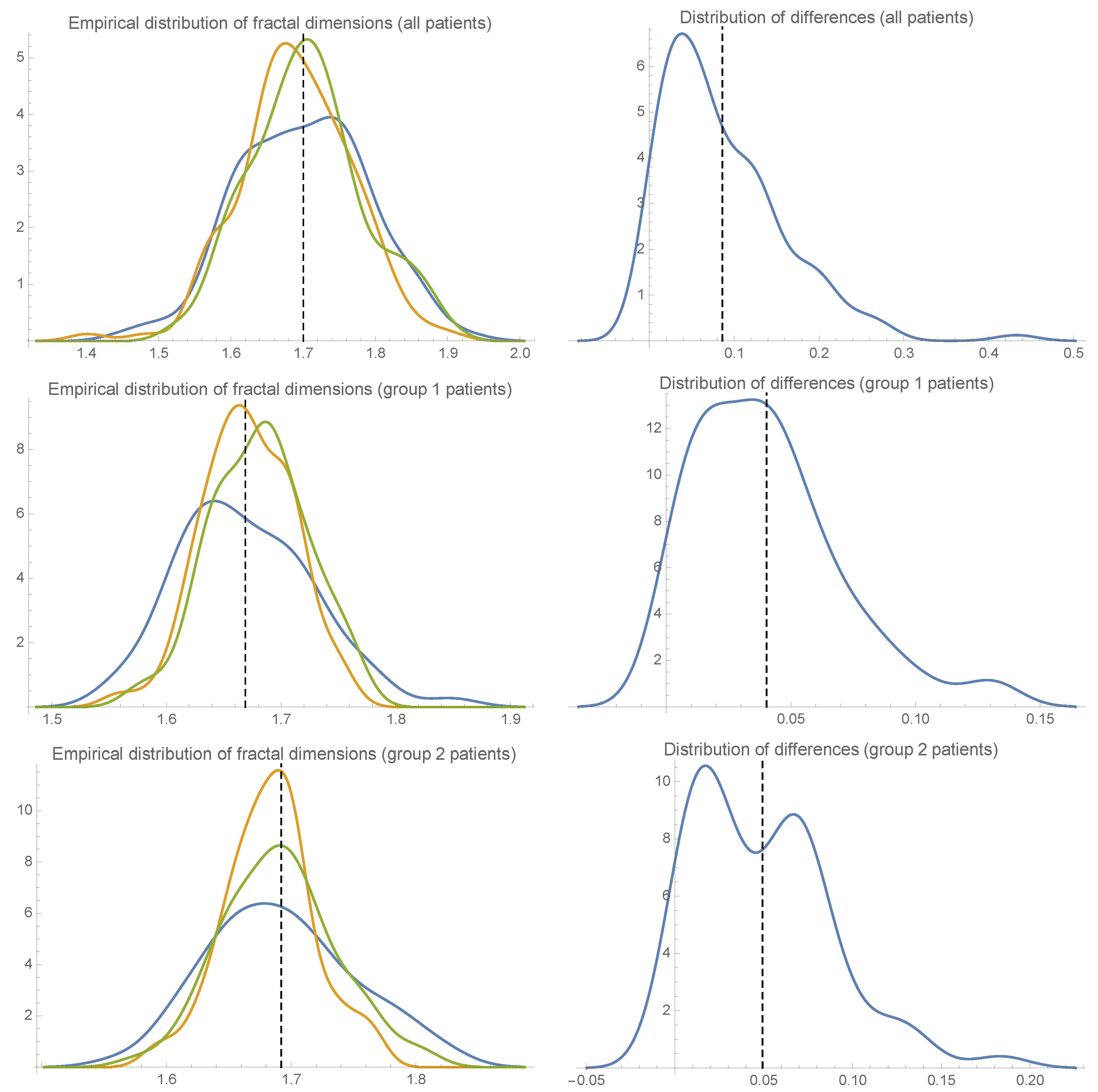
3.5. Fractal Dimension Analysis

The fractal dimensions of 130 binary images from each patient in our sample have been accurately calculated and analyzed. To deal with, an appropriate collection of scanners was selected from each patient taking part in our study. Next step was to convert such scanners to binary images by assigning “ones” to those pixels exceeding a certain color threshold and “zeros” otherwise. For illustration purposes, Figure 2 provides a graphical representation of an actual scanner from a subject that took part in our study together with its binary images for illustration purposes.
Thus, a mean fractal dimension equal to 1.70 and a standard deviation of 0.09 were found. We also extracted both left and right sides of each binary image in the sample and calculated their fractal dimensions. A mean fractal dimension equal to 1.68 and a standard deviation of 0.08 were obtained for the left side binary images. Similarly, a mean fractal dimension of 1.72 and a standard deviation equal to 0.08 were found for the right side images. The results of the fractal dimension analysis carried out for each kind of binary images and each group appear in Table 2. The differences (in absolute value) between the fractal dimensions from each left binary image and its corresponding right side one were calculated. Thus, a mean difference equal to 0.09 with a standard deviation of 0.07 were obtained. Table 3 contains the results of the analysis of the differences among the fractal dimensions of each left binary image and its corresponding right side one for each group. In addition, Figure 3 (left, first row) illustrates the empirical distribution of the fractal dimension values for all the 130 binary images analyzed as well as the empirical distribution of the fractal dimensions from their corresponding lateral binary images. In addition, the empirical distribution of the differences between each left binary image and its corresponding right side one is depicted in Figure 3 (right, first row).
To properly test the null hypothesis μ a , l μ a , r = 0 , where μ a , l (resp., μ a , r ) denotes the mean of the fractal dimensions of the right (resp., left) side binary images of the whole sample, we obtained a (medium) effect size equal to 0.50 , and hence, a statistical power of 0.85 . Thus, such a significance level becomes adequate to properly carry out such a comparison.
In this way, a p-value equal to 0.21 was found by the Mann–Whitney test when comparing the (mean of the) fractal dimension values of the left side binary images of the whole sample with respect to the (mean of the) fractal dimensions of their corresponding right side ones for all the subjects in the sample. That empirical result suggests a symmetric behavior of the fractal dimensions of the left side binary images with respect to their corresponding right side ones for all the subjects involved in the present study.
Next, we analyse in detail the fractal dimension of the binary images of the subjects from each group.

3.6. Fractal Dimension Analysis for Group One Patients

Group one consists of 65 subjects. A mean fractal dimension of 1.67 with a standard deviation equal to 0.06 was found. Moreover, we obtained a mean fractal dimension equal to 1.66 and a standard deviation of 0.04 regarding the left side binary images for all the patients assigned to group one. Similarly, a mean fractal dimension of 1.68 and a standard deviation equal to 0.04 for the right side images from the subjects in group one were obtained. Further, for each patient in group one, the differences (in absolute value) between the fractal dimension of each right side image and the fractal dimension of its corresponding left side one were analyzed. As such, a mean difference equal to 0.04 and a standard deviation of 0.03 were found. Figure 3 (left, second row) shows the empirical distribution of the fractal dimensions of all the 65 binary images of each subject in group one as well as the empirical distribution of the fractal dimensions of their corresponding lateral images. On the other hand, Figure 3 (right, second row) illustrates the empirical distribution of the differences between the fractal dimension of each left side image and the fractal dimension of its corresponding right side one for the subjects in group one.
To appropriately test the null hypothesis μ 1 , l μ 1 , r = 0 , where μ 1 , l (resp., μ 1 , r ) refers to the mean of the fractal dimensions of the right (resp., left) side binary images of group 1 subjects, we obtained a (medium) effect size equal to 0.50 , leading to a statistical power of 0.85 at a confidence level of 0.05 . As such, that significance level becomes valid to properly carry out that comparison.
A p-value equal to 0.19 was provided by the Mann–Whitney test when comparing the (mean of the) fractal dimension values of the left side binary images with respect to the (mean of the) fractal dimensions of their corresponding right side ones for all the subjects in group one. That empirical result suggests a symmetric behavior of the fractal dimensions of the left side binary images with respect to their corresponding right side ones for all the patients in group one.

3.7. Fractal Dimension Analysis for Patients in Group Two

Group two contains 65 subjects. A mean fractal dimension of 1.70 with a standard deviation equal to 0.06 was found. Moreover, we obtained a mean fractal dimension equal to 1.68 and a standard deviation of 0.04 regarding the left side binary images for all the patients assigned to group one. Similarly, they were obtained a mean fractal dimension of 1.70 and a standard deviation equal to 0.04 for the right side images from the subjects in group one. Further, for each patient in group two, the differences (in absolute value) between the fractal dimension of each right side image and the fractal dimension of its corresponding left side one were analyzed. As such, a mean difference equal to 0.05 and a standard deviation of 0.04 were found. Figure 3 (left, third row) shows the empirical distribution of the fractal dimensions of all the 65 binary images of each subject in group two as well as the empirical distribution of the fractal dimensions of their corresponding lateral images. On the other hand, Figure 3 (right, third row) illustrates the empirical distribution of the differences between the fractal dimension of each left side image and the fractal dimension of its corresponding right side one for the subjects in group two.
To properly test the null hypothesis μ 2 , l μ 2 , r = 0 , where μ 2 , l (resp., μ 2 , r ) refers to the mean of the fractal dimensions of the right (resp., left) side binary images of group 2 subjects, an effect size equal to 0.57 was obtained, leading to a statistical power of 0.85 at a confidence level of 0.05 . As such, that significance level was adequate to properly carry out such a comparison.
A p-value equal to 0.38 was provided by the Mann–Whitney test when comparing the (mean of the) fractal dimension values of the left side binary images with respect to the (mean of the) fractal dimensions of their corresponding right side ones for all the subjects in group two (at a confidence level of 95 % ). That empirical result suggests a symmetric behavior of the fractal dimensions of the left side binary images with respect to their corresponding right side ones for all the patients in group two.

3.8. Analysis of Fractal Dimension by Groups

In this section, we shall perform a series of pairwise comparisons by groups in regard to the (empirical) distribution of the (lateral) fractal dimensions of the binary images that were assigned to each of them. In fact, recall that the research question to tackle with in the present study is as follows: Are there patterns of symmetry on bone structure density over nasopalatine foramen? In this section, we provide some empirical evidence in regard to such symmetry patterns. More specifically, next we carry out all the pairwise comparisons between the fractal dimension distributions (resp., the lateral fractal dimension distributions) of the binary images from the three groups.

Fractal Dimension Comparison between Groups One and Two

Next, we compare the mean of the fractal dimensions of the whole binary images from group one patients with respect to the mean of the fractal dimensions of the whole binary images from group two patients. Figure 4 (first row) compares the empirical distributions of the fractal dimensions of all the binary images in each group.
To appropriately test the null hypothesis μ 1 μ 2 = 0 , where μ i : i = 1 , 2 denotes the mean of the fractal dimensions of the whole binary images of group i subjects, an effect size equal to 0.50 was obtained, leading to a statistical power of 0.85 at a confidence level of 0.05 . Thus, that significance level was adequate to properly carry out that comparison.
A p-value equal to 0.28 was provided by the Mann–Whitney test, which suggest that no significative differences were found.
We also compared the means of the fractal dimensions of the left side binary images from each group. Figure 4 (second row, left) depicts the empirical distributions of the fractal dimensions of the left binary images in each group.
Thus, to properly test the null hypothesis μ 1 , l μ 2 , l = 0 , where μ i , l : i = 1 , 2 denotes the mean of the fractal dimensions of the left side binary images of group i subjects, an effect size equal to 0.50 was obtained, leading to a statistical power of 0.85 at a confidence level of 0.05 . Therefore, such a significance level was adequate to properly carry out that comparison.
A p-value of 0.14 was found by the Mann–Whitney test at a confidence level of 95 % . That result throws some empirical evidence in regard to a similar behavior of the empirical distributions of the fractal dimensions of the left side binary images from both groups.
The means of the fractal dimensions of the right side binary images from each group were compared, as well. Figure 4 (second row, right) illustrates the empirical distributions of the fractal dimensions of the right binary images in each group.
Thus, to properly test the null hypothesis μ 1 , r μ 2 , r = 0 , where μ i , r : i = 1 , 2 denotes the mean of the fractal dimensions of the right side binary images of group i subjects, an effect size equal to 0.50 was obtained, which leads to a statistical power of 0.85 at a confidence level of 0.05 . Hence, that significance level was adequate to properly carry out such a comparison.
A p-value of 0.29 was found by the Mann–Whitney test at a confidence level of 95 % . Table 4 summarizes the results of the statistical comparison of means of the fractal dimensions of each kind of image and group. They suggest that the empirical distributions of the fractal dimensions of the right binary images from both groups are similar.

3.9. A Note on the Multiple Comparisons Problem

To prevent from Type I errors, we applied Bonferroni type adjustment. That procedure throws a more stringent p-value, which depends on the number of hypotheses tested, and makes it less likely to commit Type I errors. Thus, let H 1 , , H 6 be the 6 null hypotheses tested in that section. If p i denotes the (Mann–Whitney) p-value for testing the null hypothesis H i , Bonferroni procedure states that H i has to be rejected whenever p i 1 6 α , where α = 0.05 is the significance level considered throughout this article. In this way, the p-value provided by Bonferroni approach is α B = 0.01 . Since all the (Mann–Whitney) p-values calculated (c.f., e.g., Table 4) stand > α B , we discard significative effects from Type I errors.
On the other hand, recall that type II error consists of accepting the null hypothesis when it is actually false. Since statistical power is the probability of rejecting the null hypothesis when it is false, then we have that statistical power = 1 β , where β denotes the probability of type II error. In this paper, we tested the null hypothesis μ i = μ j with i , j = 1 , 2 , 3 and i j , where μ i denotes the mean of the fractal dimensions of the binary images from all the patients in group i. To deal with, a significance level α = 0.05 was selected and our sample consisted of two groups containing 65 patients each. As stated in the previous revision of our article, a statistical power of 0.85 was obtained by such an experimental design. Hence, β = 0.15 is the probability of type II error in this study, i.e., the probability of accepting that null hypothesis when it is actually false equals 15 % . An option to reduce that β would consist of increasing the sample size in further studies. Indeed, that way would allow us to hold α at the desired level while still reducing β . As such, the statistical power of our study would increase.

4. Conclusions

All the anatomical considerations that surround the nasopalatine foramen have been described in this paper. Regarding them, an analysis of bone density via an efficient calculation of fractal dimension has been carried out in that area. A sample with 130 patients was considered. 65 of them were assigned to group one (without loss of teeth) and 65 to group two (with the absence of some teeth). 63 women took part in the final stage of our study. The mean age of the patients was equal to 53.16 years with a standard deviation of 8.73 years. For each subject, cone beam computed tomography was performed for treatment needs. A specific window, which coincides with an axial cut at the level of the anterior nasal spine, was selected. In that area, different anthropometric measurements were performed. In addition, we applied a novel and accurate approach to calculate the fractal dimension of binary images generated from each patient CBCT scanner. Three types of binary images were used for each subject including both right and left sides from the original one. Mann–Whitney tests threw some statistical evidence regarding a symmetric behavior of such binary images. Moreover, we found no significative differences regarding the anthropometric measures explored in the different groups of our study. Accordingly, several patterns of symmetry were appreciated at a complete range of levels.
In this paper, we highlight the utility of an accurate fractal dimension model as a reliable and unbiased approach for clinicians to analyse the density of the bone structure through CBCT images from a large sample of patients. In this way, it becomes a reproducible and non-invasive tool to properly quantify the bone structure density. Advanced surgical techniques for maxilla reconstruction need stable anatomic measures allowing the assessment of both morphological and structural characteristics of a given zone with the aim to perform minimally invasive interventions and with the best functional and aesthetic results, that have a positive impact on the quality of life of patients.
Mathematics provides the natural environment for modelling and analyzing problems from different areas in particular from health sciences, see for instance some applications to the war against cancer like [12,13]. In the next Appendix A we shall present all mathematical machinery used in this work.

Author Contributions

All authors of this paper have contributed in an equal way to the results presented.

Funding

This paper has been partially supported by grant No. MTM2015-64373-P (MINECO/FEDER, UE), MINECO grant number MTM2014-51891-P and Fundación Séneca de la Región de Murcia grant number 19219/PI/14.

Acknowledgments

The authors would like to express their gratitude to anonymous reviewers whose suggestions, comments, and remarks have allowed them to enhance the quality of this paper.

Conflicts of Interest

The authors declare no conflict of interest.

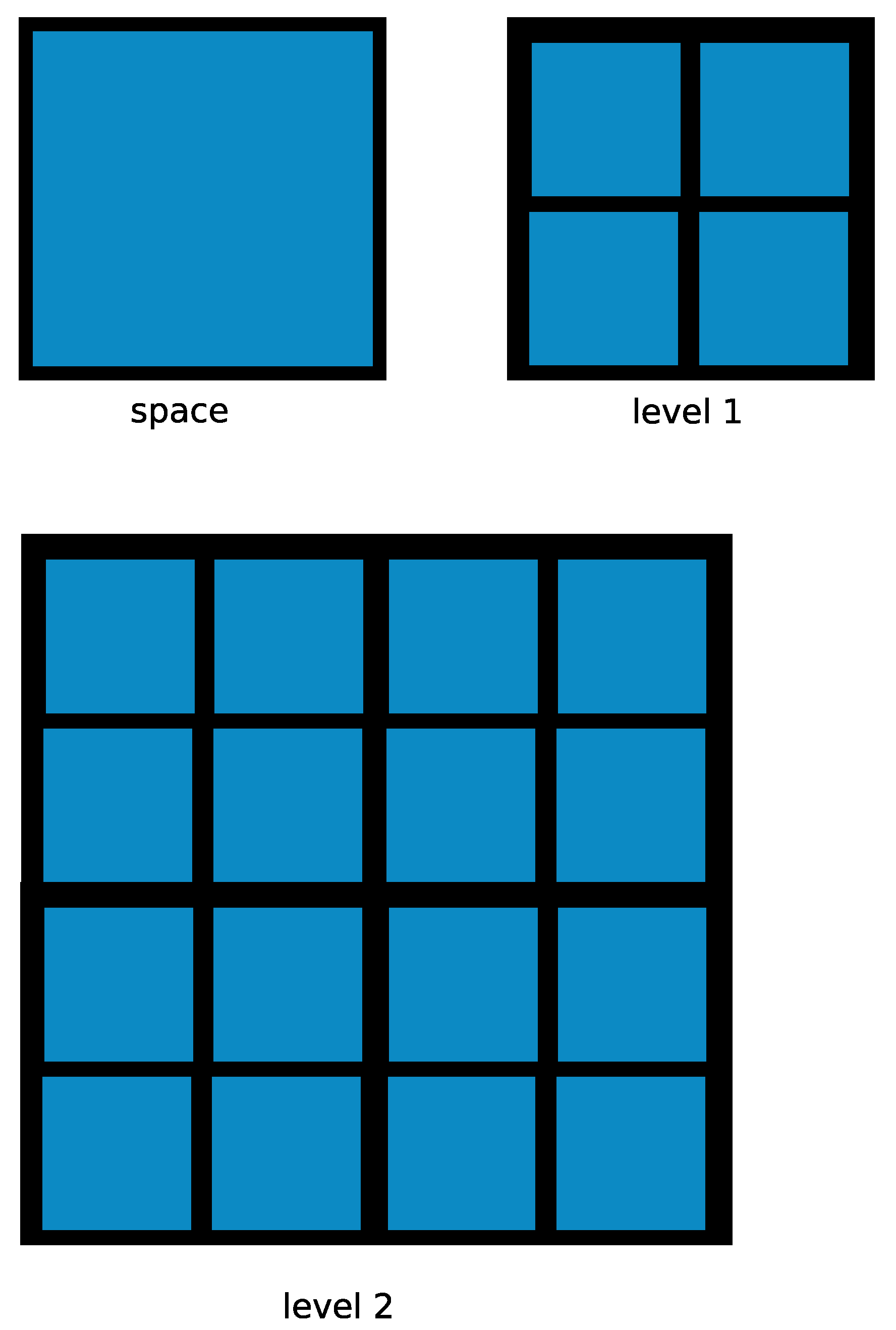
Appendix A. Mathematical Foundations on Fractal Dimension Calculations

This appendix contains the mathematical framework including notations, notions, theoretical results, and main ideas we applied to efficiently deal with the calculations of the fractal dimensions of CBCT images in this paper. We would like to highlight the role of the concept of fractal structure (c.f. upcoming Definition A2) to accurately deal with such calculations. As such, Theorem A1 is the key result applied throughout this work in regard to fractal dimension computations.
Let δ > 0 . A (plane) δ –cube is a set of the form [ δ k 1 , δ ( 1 + k 1 ) ] × [ δ k 2 , δ ( 1 + k 2 ) ] , where k 1 , k 2 Z . The standard definition of box dimension (for plane subsets) is provided below.
Definition A1.
Let F R 2 . Its (lower/upper) box dimension is given by
dim ̲ B ( F ) = lim ̲ δ 0 log N δ ( F ) log δ .
dim ¯ B ( F ) = lim ¯ δ 0 log N δ ( F ) log δ .
In particular, the box dimension of F, dim B ( F ) , is defined through the following limit (if it exists):
dim B ( F ) = lim δ 0 log N δ ( F ) log δ ,
where N δ ( F ) can be calculated as the number of δ –cubes that intersect F.
The utility of box dimension lies in the fact that it can be easily calculated in empirical applications (mainly on Euclidean spaces) involving fractal dimension. In fact, it can be estimated as the slope of a regression line to compare log δ vs. log N δ ( F ) over a discrete collection of scales properly chosen.
Another key concept to tackle with fractal dimension calculation is fractal structure. First, we recall that a covering of a set X is a collection of subsets, Γ , such that X = { A : A Γ } .
Definition A2.
Let Γ = { Γ n : n N } be a countable family of coverings of a given set X. We shall understand that Γ is a fractal structure provided that the two following statements hold:
(i) 
for each A Γ n + 1 , there exists B Γ n such that A B .
(ii) 
B = { A Γ n + 1 : A B } for all B Γ n .
It is worth mentioning that covering Γ n of Γ is called as level n of that fractal structure. Equivalently, Definition A2 states that level n + 1 is a strong refinement of level n of Γ . Additionally, the levels of the natural fractal structure on R 2 , Δ = { Δ n : n N } , are defined as
Δ n = k 1 2 n , 1 + k 1 2 n × k 2 2 n , 1 + k 2 2 n : k 1 , k 2 Z .
In particular, the natural fractal structure on R 2 can be induced on the unit square by defining
Δ n = k 1 2 n , 1 + k 1 2 n × k 2 2 n , 1 + k 2 2 n : k 1 , k 2 = 0 , 1 , , 2 n 1
The first two levels of the natural fractal structure on [ 0 , 1 ] × [ 0 , 1 ] are depicted in Figure A1.
Figure A1. First two levels of the natural fractal structure on [ 0 , 1 ] × [ 0 , 1 ] . Notice that the first level consists of four squares with sides equal to 1 2 , Γ 2 contains 4 2 squares with sides equal to 1 2 2 , and in general, level n consists of 4 n squares with sides equal to 1 2 n .
Symmetry 11 00202 g0a1
In this paper, we shall apply the following result to efficiently calculate the box dimension of a binary images from the CBCT scanner of each patient. Observe that it suffices with calculating the number of δ -cubes that intersect α 1 ( F ) [ 0 , 1 ] for (lower/upper) dim B ( F ) calculation purposes.
Theorem A1
(c.f. Corollary 2.6 in [14]). Let Δ be the natural fractal structure on [ 0 , 1 ] × [ 0 , 1 ] and assume that [ 0 , 1 ] is endowed with the fractal structure Γ with levels given by Γ n = { [ k 2 2 n , 1 + k 2 2 n ] : k = 0 , 1 , , 2 2 n 1 } . In addition, let F be a subset of [ 0 , 1 ] × [ 0 , 1 ] and α : [ 0 , 1 ] [ 0 , 1 ] × [ 0 , 1 ] a function with Δ = α ( Γ ) . The (lower/upper) box dimension of F can be calculated by the following expressions:
dim ̲ B ( F ) = 2 · lim ̲ δ 0 log N δ ( α 1 ( F ) ) log δ .
dim ¯ B ( F ) = 2 · lim ¯ δ 0 log N δ ( α 1 ( F ) ) log δ .
In particular, if there exists dim B ( F ) , then we have
dim B ( F ) = 2 · lim δ 0 log N δ ( α 1 ( F ) ) log δ .
To deal with the construction of the curve α , we refer the reader to ([14], Section 2.4). For additional details regarding this mathematica invariant, we refer the reader to [15].

References

  1. Gómez de Ferraris, M.E.; Campos Muñoz, A. Histología, Embriología e Ingeniería Tisular Bucodental; Panamericana: Madrid, Spain, 2009; ISBN 978-607-7743-01-9. [Google Scholar]
  2. Velayos Santana, J.L. Anatomía de la Cabeza para Odontólogos; Panamericana: Madrid, Spain, 2007; ISBN 978-84-9835-068-5. [Google Scholar]
  3. López Muñiz, A.; Hernández González, L.C.; del Valle Soto, M.; Suárez Garnacho, S.; Carbajo Pérez, E.; Junceda Moreno, J. Anatomía Topográfica Humana; Ediciones de la Universidad de Oviedo: Oviedo, Spain, 2008; ISBN 978-84-7468-911-2. [Google Scholar]
  4. Nart Molina, J.; Marcuschamer Gittler, E.; Rumeu Milá, J.; Santos Alemany, A.; Griffin, T.J. Preservación del reborde alveolar. Por qué y cuándo. Periodoncia y Osteointegración 2007, 17, 229–237. [Google Scholar]
  5. Chimenos Kustner, E.; Ribera Uribe, M.; López López, J. Gerodontología; Sociedad Española de Gerodontología: Santiago de Compostela, Spain, 2012; ISBN 978-84-695-3382-6. [Google Scholar]
  6. Misch, C.E. Contemporary Implant Dentistry; Mosby Elsevier: St. Louis, MI, USA, 2008; ISBN 978-0-323-04373-1. [Google Scholar]
  7. Shah, N.; Bansal, N.; Logani, A. Recent advances in imaging technologies in dentistry. World J. Radiol. 2014, 6, 794–807. [Google Scholar] [CrossRef] [PubMed]
  8. Bornstein, M.M.; Balsiger, R.; Sendi, P.; von Arx, T. Morphology of the nasopalatine canal and dental implant surgery: A radiographic analysis of 100 consecutive patients using limited cone beam computed tomography. Clin. Oral Implants Res. 2011, 22, 295–301. [Google Scholar] [CrossRef] [PubMed]
  9. Liang, X.; Jacobs, R.; Martens, W.; Hu, Y.Q.; Adriaensens, P.; Quirynen, M.; Lambrichts, I. Macro- and micro-anatomical, histological and computed tomography scan characterization of the nasopalatine canal. J. Clin. Periodontol. 2009, 36, 598–603. [Google Scholar] [CrossRef] [PubMed]
  10. Hakbilen, S.; Magat, G. Evaluation of anatomical and morphological characteristics of the nasopalatine canal in a Turkish population by cone beam computed tomography. Folia Morphol. 2018, 77, 527–535. [Google Scholar] [CrossRef] [PubMed]
  11. Ruttimann, U.E.; Webber, R.L.; Hazelrig, J.B. Fractal dimension from radiographs of peridental alveolar bone. Oral Surg. Oral Med. Oral Pathol. 1992, 74, 98–110. [Google Scholar] [CrossRef]
  12. Pérez-García, V.M.; Fitzpatrick, S.; Pérez-Romasanta, L.A.; Pesic, M.; Schucht, P.; Arana, E.; Sánchez-Gómez, P. Applied mathematics and nonlinear sciences in the war on cancer. Appl. Math. Nonlinear Sci. 2016, 1, 423–436. [Google Scholar] [CrossRef]
  13. Rojas, C.; Belmonte-Beitia, J. Optimal control problems for differential equations applied to tumor growth: State of the art. Appl. Math. Nonlinear Sci. 2018, 3, 375–402. [Google Scholar] [CrossRef]
  14. Fernández-Martínez, M.; Gómez García, F.J.; Sánchez Guerrero, Y.; López Jornet, P. An intelligent system to study the fractal dimension of trabecular bones. J. Intell. Fuzzy Syst. 2018, 35, 4533–4540. [Google Scholar] [CrossRef]
  15. Fernández-Martínez, M. A survey on fractal dimension for fractal structures. Appl. Math. Nonlinear Sci. 2016, 1, 437–472. [Google Scholar] [CrossRef]
Figure 1. Cutting selection to be studied and taking measurements.
Symmetry 11 00202 g001
Figure 2. Graphical representation of an actual cone beam computed tomography (CBCT) from a patient that took part in our study (left) and its corresponding binary images.
Symmetry 11 00202 g002
Figure 3. The blue line in each plot at the left illustrates the empirical distribution of the fractal dimension values for all the binary images analyzed from each group in our patient sample. Further, the discontinuous line marks the mean fractal dimension of the binary images from all the scanners analyzed. Notice also that the orange line (resp., the green line) represents the empirical distribution of the fractal dimensions of the left side (resp., the right side) binary images from each group of patients. On the other hand, each graph at the right depicts the empirical distribution of the differences (in absolute value) between each left side binary image and its corresponding right side one from each group of patients. The discontinuous line represents the mean of such differences.
Symmetry 11 00202 g003
Figure 4. Empirical distributions of the fractal dimensions of the binary images from both groups one (blue line) and two (picture at the first row) and empirical distributions of the fractal dimensions of their lateral binary images (second row). The discontinuous straight lines mark the mean fractal dimension of each group and each kind of binary images.
Symmetry 11 00202 g004
Table 1. Sample description by attributes. Recall that DCV denotes distance anterior wall nasopalatine hole to anterior nasal spine, DCP means distance back wall foramen (NF) to border palate bone, DVD is distance right side wall NF to right canine mamelon, DVI refers to distance left lateral wall NF to left canine mamelon, Area is the area of the NF, and W, H, mean, and standard deviation are provided by the software.
Whole Sample (n = 130)Female Group (n = 68)Male Group (n = 62)
AttributeMeanStd. Dev.MeanStd. Dev.MeanStd. Dev.
Age53.678.2054.628.9953.037.05
DCV7.541.537.291.638.751.35
DCP3.991.654.051.694.131.26
DVD12.951.7512.821.6213.711.96
DVI12.981.3412.381.6213.131.70
Area5.632.185.331.985.182.60
W2.960.713.030.722.640.73
H2.230.592.260.442.010.66
Mean158.66120.83142.65107.52160.1698.83
DIM1.690.091.680.131.690.10
Table 2. Results of the fractal dimension analysis for each kind of binary images and group.
Dim. of Binary ImagesDim. of Left ImagesDim. of Right Images
nMeanStd. Dev.MeanStd. Dev.MeanStd. Dev.
Whole sample1301.700.091.680.081.720.08
Group One651.670.061.660.041.680.04
Group Two651.700.061.680.041.700.04
Table 3. Analysis of the differences among the fractal dimensions of each left binary image and its corresponding right side one for each group.
Differences (in abs.) among Left and Right DIMs
MeanStd. Dev.Mann–Whitney (p-Value)
Whole sample0.090.070.21
Group One0.040.030.19
Group Two0.050.040.38
Table 4. Comparison of empirical distributions of (lateral) fractal dimensions from each group. They are provided the p-values from the Mann–Whitney tests involving both groups. No significative differences were found at a confidence level of 95 % .
Group One vs. Two Comparison
CBCT imagesM-W p-Value
Whole images0.28
Left images0.29
Right images0.19

