Dynamic Vehicle Routing Problem—Predictive and Unexpected Customer Availability

Abstract

The Dynamic Vehicle Routing Problem (DVRP) is one of the most important problems in the area of enterprise logistics. DVRP problems involve these dynamics: the appearance of customers, travel times, service times, or vehicle availability. One of the most often considered aspects of the DVRP is the availability of customers, in which a part or all of the customers are revealed dynamically during the design or execution of the routes. A classification of the DVRP problem due to various elements causing dynamism is proposed. The aim of the paper is to distinguish dynamic VRP, which takes into account the dynamic appearance of customers to serve during the design or execution of the routes. In particular, the difference between the predictive and unexpected aspects of the customer’s availability is considered. Above all, the variant of customer’s availability which is predicted according to an appropriate general rule is modeled using the algebraic-logical meta-model (ALMM). It is a methodology which enables making collective decisions in successive process stages, not separately for individual vehicles. The algebraic-logical model of the dynamic vehicle routing problem with predicted consumer availability is proposed. The paper shows the possibilities of applying the ALMM approach to dynamic problems both with predicted and unexpected customer availability.

1. Introduction

The basic Vehicle Routing Problem (VRP) consists in an efficient set of multiple routes for a fleet of vehicles that all start and end at a central depot to service a given set of customers (e.g., warehouses, stores, schools, cities), when each customer should be visited once by only one vehicle at the lowest cost. Thus, all data is known in advance, i.e., it is a static problem.

The real logistic and manufacturing problems are one of the most challenging because the large number of them is dynamic. In general, in the dynamic problem, a part or all of the input data is revealed dynamically during the design or implementation of a statically planned solution. Dynamic problems are much harder to solve than static combinatorial optimization problems, where all data are known in advance, i.e., before the optimization process has started. The Dynamic Vehicle Routing Problem (DVRP) is one of the important variants of VRP. Its aim consists in designing the optimal set of routes for a fleet of vehicles in order to serve a given set of customers while new customer orders arrive during the performance of the planned earlier work day. Thus, routes must be reconfigured dynamically while executing the current simulation [1]. The supply and distribution companies, courier services, transport of disabled people and medical emergency services are examples of real-life DVRP applications.

In the literature, the Vehicle Routing Problem (VRP) problems are widely discussed and a number of variants of classical VRP have been studied. The most popular variant is Capacitated VRP (CVRP), where each customer has a demand for good and vehicles have the finite capacity [2,3]. Second is the VRP with Time Windows (VRPTW), where each customer must be visited during a specific time frame [4]. If goods have to be picked up and delivered in specific amounts at the vertices, it means the Pick-up and Delivery VRP (PDP-VRP) [5]. In particular, the Vehicle Routing Problem with Simultaneous Pickup and Delivery (VRPSPD) considers clients that require pick-up and delivery service simultaneously [6,7]. The Heterogeneous fleet VRP (HVRP) denotes different capacities of vehicles [8,9,10,11]. In particular, the paper [8] presents heterogeneous VRP review, including classification, considerable input data characteristics, and decision making approaches, and heuristic and meta-heuristics algorithms. Routing problems that involve moving people between locations are referred to as Dial-A-Ride-Problem (DARP) [12,13] or Dial-A-Flight-Problem (DAFP), for air transport [14].

The DVRP is an NP-hard optimization problem. Because of that, the exact optimization techniques are not used effectively to solve it and usually approximate methods are used, although they do not guarantee an optimal solution. Dynamic problems have usually been solved using re-optimization (periodic re-optimization or continuous re-optimization) or fast insertion techniques heuristics with background optimization techniques [15]. The periodic re-optimization approaches start at the beginning of the day with a first optimization that produces an initial set of routes. Then, an optimization procedure periodically solves a static problem corresponding to the current state, either whenever the available data changes or at fixed intervals of time [16]. In continuous re-optimization approaches, the optimization is performed throughout the day. The information on good solutions is stored in an adaptive memory. Whenever the available data changes, a decision procedure aggregates the information from the memory to update the current routing [17].

The optimization techniques include meta-heuristics, for example, Genetic Algorithm (GA), Ant Colony System (AS), Multi-Particle Swarm Optimization (MAPSO), and Tabu Search (TS). In particular, DVRP can be considered as an extension to the standard VRPs that is created by decomposing a DVRP into a sequence of static VRPs [18]. Metaheuristics for Dynamic Vehicle Routing are described in the paper [1]. The authors deal with two methods of solving the problem: population-based metaheuristics (e.g., Ant Colony, Evolutionary Algorithms, and Particle Swarm Optimization) and trajectory-based metaheuristics (e.g., Tabu Search, Greedy Randomized Adaptive Search Procedure (GRASP), variable neighborhood search). Also, a number of real-life applications and dynamic performances measures of different metaheuristics are described. The approaches based on dynamic programming could be also classified as trajectory based simulations [19,20]. In [21] DVRP is solved using an enhanced Genetic Algorithm (GA) that tries to increase both diversity and the capability to escape from local optima.

Moreover, there are also dynamic problems where the existence of the input data is known but the exact time of their availability is not known in advance. This availability may depend on the state of the system and can be determined using a general rule specifying any dependencies between input data (for example rule according to which it can be determined from when it is possible to deliver to the given company). It is impossible to determine a priori values of all variables and parameters for this class of problems. In such problems, not all decisions are possible at every stage due to the existing constraints or dynamic input data. In consequence, it is hard or impossible to simply implement the improvement algorithms because a significant number of obtained solutions will not be allowed. Thus, such problems require a distinct approach that allows one to construct the solution sequentially and significantly reduce the number of impossible solutions. The decision-making process should be carried out in stages. An approach that meets these needs is the Algebraic-Logical Meta-Model (ALMM). The ALMM approach is based on a multistage decision-making process, where the decision is made jointly and considers the current situation (current process state). It is a trajectory-based simulation. Previously, the ALMM approach has been used for a dynamic vehicle routing problem [22] and the supply routes for a multi-location companies problem [23]. This paper presents an approach based on the ALMM methodology for a dynamic vehicle routing problem with the possibility of modeling the dynamic predictive events, in particular, the appearance of new customers to visit during the simulation according to an appropriate general rule.

The main contributions of this paper are as follows:

• supplementing and refining the classification of problems related to dynamic elements related to customers;
• presenting the possibilities of applying the Algebraic-Logical Meta-Model approach to dynamic problems where input data availability may depend on the state of the system and can be determined by a special rule. In particular, collective decision making in dynamic vehicle routing problems with predicted consumer availability is proposed;
• presenting the possibilities of applying the Algebraic-Logical Meta-Model approach to dynamic problems with unexpected customer availability;

The remainder of the paper is structured as follows. Section 1.1 reviews the literature of dynamic elements in VRP. Section 2 presents predictive and unexpected events in Dynamic VRP. The definition and features of Algebraic-Logical Meta-Model are presented in Section 3. Section 4 includes the description and formulation of the DVRP with predicted consumer availability. The particular elements of an algebraic-logical model of DVRP with predicted consumer availability are described in Section 5. In particular, an opportunity to model the problem with unexpected customer availability is proposed in Section 5.9. Section 6 presents the additional remarks connected with additional prediction, followed by discussion in Section 7.

1.1. Dynamic Elements in Vehicle Routing Problems

There are various reasons for changing the input data in Dynamic VRP. It is possible to define several dynamic features which cause dynamism in the classical VRP. It should be emphasized that various dynamic features imply a set of different Dynamic VRPs. The most often considered are uncertain inputs (e.g., new requests or cancellations can happen at any time, customers could modify size or deadline of their orders, the travel time for some routes could be increased due to a traffic accident) or stochastic inputs (e.g., customer demands are represented by random variables).

An extensive review of the DVRP literature has been presented by the Pillac at al. in [16]. The authors have introduced the notion of degree of dynamism. Additionally, a comprehensive review of applications and solution methods for dynamic vehicle routing problems is presented. Moreover, the authors draw attention to the need to introduce the taxonomy of dynamic vehicle routing problems. Thanks to this, more precise classification of approaches, evaluation of similarities between problems, and fostering the development of generic frameworks would be possible. An attempt to create such a taxonomy was taken in [24]. Psaraftis at al. have develop a taxonomy of DVRP papers according to 11 criteria: type of problem, logistical context, transportation mode, objective function, fleet size, time constraints, vehicle capacity constraints, the ability to reject customers, the nature of the dynamic element, the nature of the stochasticity, and the solution method.

A short overview of vehicle routing variants and a classification depending on the nature of the available data is presented in [15]. A short summary of various algorithms for solving dynamic and stochastic VRPs is included. Additionally, VRP with Stochastic Customers is described, where not all customer requests are known a priori, but stochastic information about the expected number of customer requests is considered. The dynamically revealed demand for a set of known customers is another example of DVPR. An example is a problem where customers’ demands follow known probability distributions and a customer’s actual demand is only revealed when the vehicle arrives at the customer location [20]. Another variant of dynamic stochastic VRP is presented in [25]. Authors also consider customers whose demand is known only when the vehicle arrives at them and they should be visited based on the sequence of the a priori tour, but additionally, the final route includes returns to the depot when the vehicle needs replenishment. The decision about replenishment depends on the demand of the next customer. Furthermore, dynamic VRP where customers’ demand distribution is unknown and not certain is discussed in [26].

Also, dynamic pickup and delivery problem with impatient customers is considered [27]. The fleet of vehicles transports a good from a pickup location to a delivery location. The vehicles have a unitary capacity. Each customer may cancel the request if the good is not picked up before a deadline. It is considered that the deadline is stochastic, requests’ arrival time and locations are distributed according to a certain stochastic process and the requests’ information is disclosed only at the arrival time.

VRP becomes Vehicle Routing Problems with Uncertainty (VRPU) when one or both of demand and edge costs, including transportation cost and travel time, are uncertain. The optimization approach for solving VRPU includes stochastic and robust optimization approaches [28]. A robust vehicle routing problem with hard time windows, in which travel times are considered uncertain due to potential delays based on weather conditions, port congestion or strikes, or mechanical problems, is presented in [29]. Moreover, more than fifty articles of stochastic VRPs have been described in [30]. The uncertain data was categorized into four stochastic factors: customer demand, travel time, customers, and service time.

An interesting example of a dynamic VRP is a vehicle routing with cross-docking [31,32]. A fleet of vehicles leaving from the cross-dock takes routes to visit backhaul suppliers to pick-up the ordered goods, then returns to the cross-dock. The delivered goods are sorted according to the orders and distributed to the destination customers. In the presented version, it is assumed that at the cross-docking stage the arrival time of all inbound vehicles is equal to the departure time of all outbound vehicles. The problem becomes even more complicated when these times are different and also the cross-docking capacity is limited. Then it is a problem in which decisions are made depends on the state of the system.

Finally, the source of dynamism is vehicle availability, the possible breakdown of vehicles for example. Tabu Search algorithms are developed to solve the problem of a vehicle breaks down during the delivery to minimizing the costs is considered in [33]. The multiple-depot vehicle type rescheduling problem (MDVTRSP) is a dynamic extension of the classic multiple-depot vehicle scheduling problem (MDVSP), where a heterogeneous fleet is considered in [34]. The authors consider the breakdown of vehicles and the need to create a new schedule by minimizing transportation costs and deviations from the original plan. The paper [35] introduces and studies real-time vehicle rerouting problems with time windows that undergo service disruptions due to vehicle breakdowns. A Lagrangian relaxation based-heuristic has been developed for solving the vehicles rerouting problem with the objective of minimizing a weighted sum of operating, service cancellation, and route disruption costs.

2. Predictive and Unexpected Events in Dynamic VRP

The various dynamic features imply a set of different Dynamic VRPs. Proper classification of the problem is very important for the selection of the solution method, and for dynamic problems, it is important to determine the type of dynamism. It may result, among others, from an availability of information which can distinguish two main types: locally available information (e.g., a number of available vehicles, a demand of a certain customer) and globally available information (e.g., current traffic intensity in the city traffic from the GPS, news about a road closure due to an accident broadcasted by radio).

Nature of Dynamic VRP is different and it depends largely on the element issues. One of the most often considered aspects of the dynamic problem DVRP is the availability of recipients. According to [36] some 80% of the problems involve the dynamic appearance of customers, whereas some 10% involve dynamic travel times, and some 3% consider vehicle break-downs. Nevertheless, the taxonomy of dynamic vehicle routing problem presented in Section 2 is not comprehensive and should be supplemented with more detailed information on the nature of customer dynamism. Thus, the following dynamic elements should be distinguished:

• dynamic consumers—the information about customers is revealed gradually and concurrently with actual route execution. In particular, the changes regarding consumers are related to
  • dynamic requests, including new requests and requests cancellations
  • dynamic localization, including changes in customers locations
  • dynamic demands, including changes in the number of ordered goods
  • dynamic customers’ availability—changing the time window of the consumer’s availability (soft time window or hard window) and the information on which customers are present is unknown a priori
  • dynamic order time—including changes in required by the customer serving or delivery time (customers usually speed up the serving or delivery deadline)
• dynamic travel—travel times can be time or environment dependent, e.g., weather or traffic conditions delay arrival at the given customer
• dynamic service times—the planned repair time may change depending on the problems identified on the site
• dynamic vehicle availability, including unexpected events like vehicle breakdowns

2.1. Dynamic Customers’ Availability

One of the important aspects of a dynamic problem is information about costumer’s availability. In static problems quality of information about costumer’s availability is known (deterministic), i.e., the customer is available all the time, the exact start time of availability or the time window of availability is known. There are various reasons for the dynamically changing availability of recipients. The predictive and unexpected events related to the availability of consumer should be considered. Firstly, there are many dynamic problems which consider knowledge on the dynamically revealed information to anticipate the future (they deal with predictive events) and predictive analytics can be used to accurately forecast future data. In this case, consumer availability can be determined as follows:

• stochastic—information about possible future events and progress can be based on historical data and described by probability distributions;
• calculated based on the given rules and restrictions of the problem;

Secondly, the availability of customer may result from an unexpected event. For example, new requests that can appear dynamically during the day can be treated as a new availability of customer. Then, because of the owned information, two types of customers should be distinguished:

• well-known customer—all data describing the consumer is known, i.e., customer location and data on roads leading to it;
• new unknown customer—it requires new knowledge of the customer location and data on roads leading to it—the data of the problem has to be supplemented; this can be possible thanks to technological advances (Electronic Data Interchange (EDI), positioning systems like GPS or Gallileo, Geographic Information Systems (GIS), Intelligent Vehicle Highway Systems (IVHS), mobile communication systems and mobile internet, traffic information systems). These technologies increase both the availability and quality of information on future inputs.

2.2. Determining the Availability Time of Customers

The time of customer’s availability may be known in advance, unknown but depend on various constraints or dependency, or unexpected. If the availability of customers is known in advance, we are dealing with a static and deterministic problem. On the other hand, if the customer placed an order, but the time of its availability has not been provided, then it is possible to distinguish between situations where this time can be calculated based on the given rules and restrictions of the problem or stochastically predict based on historical data if only future events and progress can be determined by probability distributions ${\phi }_{n_j}\left(t\right)$.

Therefore, you can consider the following cases of determining the availability of customers:

• all customers are available from the beginning. It does not change.
• customers are not available at the beginning, but each of them has a specific time from which they will be available and the release time $r_{n_j}$ is known in advance.
• customers are not available at the beginning and their time of availability is not given in advance due to the existing dependencies. A general rule $\rho$ according to which we can determine the customer availability is known. A customer is available since the conditions of availability are met. Thus, availability start time depends on the state of system $s$ and is appropriately denoted $r_{n_j}\left(s\right)$.
• customers are available only in the time windows, known in advance $\left[r{1}_{n_j},r{2}_{n_j}\right]$.
• customers are not available at the beginning and their time of availability or time window are not given in advance, but for each of them, we have historical data on the basis of which we can predict customer behavior in this area. The availability start time and the end of availability time are predicted using probability distributions ${\phi }_{n_j}\left(t\right)$ and are appropriately denoted $\widetilde{r{1}_{n_j}}$ i $\widetilde{r{2}_{n_j}}$. These values are determined appropriately considering the confidence interval.

The problem of predicted consumer availability according to general rule $\rho$ (case 3) is considered in the paper. You can also notice that (1) and (2) are its special cases. The problem with time windows (cases 4 and 5) is not considered in this work due to its specificity. It will be the subject of separate work.

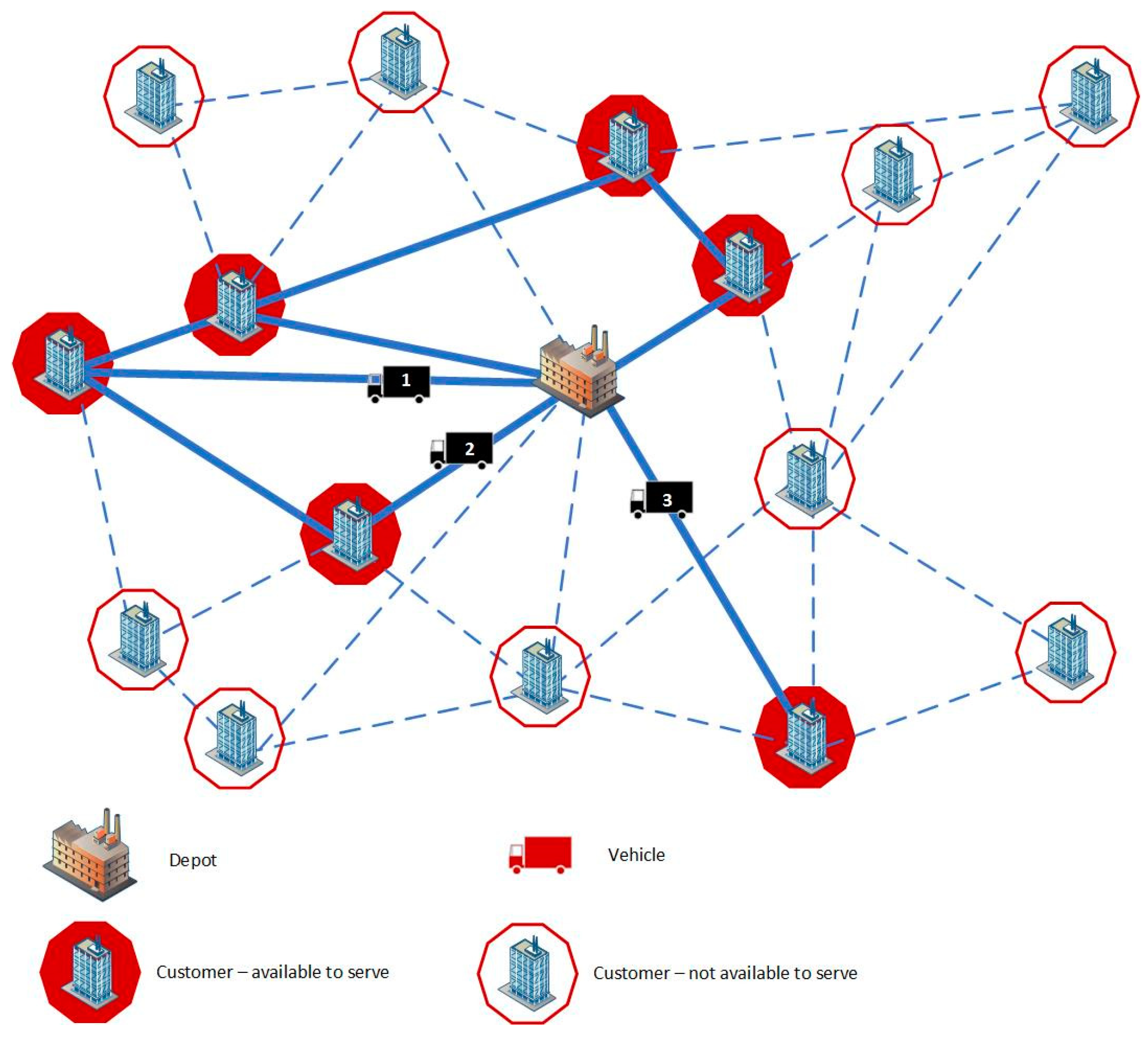
To better understand the class of dynamic problem under consideration (what we mean by dynamic), let’s consider an example of a company for which fifteen customers from all regular customers placed an order on a given working day. The customers may be served by three vehicles. The rule $\rho$ means that after serving the given customer by any vehicle, customers associated with the visited customer are available (previously unavailable). In the initial situation, only six out of fifteen customers are available to serve. Figure 1 illustrates the situation where three vehicles go to designated customers, three out of six available. Whereas, Figure 2 illustrates the next situation where customer service by a second vehicle results, according to given rule $\rho$, in the possibility of servicing another three customers, i.e., three additional clients are available now.

An example is a problem of providing services to multi-location companies. There is a need to visit the head office first (for example in order to negotiate, to establish the transaction conditions) before servicing branch offices. A branch office of a given company can be visited only if the head office of this company is already visited. However, after the head office has been visited, any salesperson from the team can visit any branch office of that company. Another example is hospital-internal logistics services, where the performance of certain subsequent services and tests is possible after sharing the results of research from other places.

Another example of a problem belonging to the considered class is a dynamic pickup and delivery problem with impatient customers, where each customer may cancel the request if the goods are not picked up before a deadline. But unlike the problem presented in [27] the deadline is determined directly by the customer (is deterministic). The customers’ location and request are known in advance (is not stochastic), but a decision in each state depends not only on previously taken decisions and also on exceeded deadlines.

3. Algebraic-Logical Meta-Model

The dynamic problem should be solved by approach considering the limitations related to the input data availability or dependencies between input data resulting from the state of the system. Methods that do not consider the possibility of changing input data cannot be used. Therefore, most dynamic approaches allow calculating the solution in the new state of the problem (including new data) and they use heuristic methods. Approaches for dynamic and deterministic vehicle routing problems can be divided into two categories: those based on periodic re-optimization, and those based on continuous re-optimization [36].

In this paper, an ALMM-based approach for collective decision making in dynamic vehicle routing problem is presented. ALMM (Algebraic-Logical Meta-Model) approach is based on a multistage decision-making process, where the decision is made jointly and considers the current situation (current process state). This approach is the process trajectory-based simulation, where the solution is constructed in stages. Thus, there is a possibility to consider the existing constraints or dynamic input data at a stage (given state of the problem). Let us recall Algebraic-Logical of Multistage Decision Process (AL of MDP) formal definition, devised by Dudek-Dyduch [37,38].

AL of MDP Definition.

Algebraic-logical of the multistage decision process is a process that is defined by the sextuple:

$$AL-MDP=\left(U,S,s_0,f,S_N,S_G\right)$$

(1)

where:

• $U$ is a set of decisions,
• $S=X\times T$ is a set of generalised states ($X$ is a set of proper states and $T\subset {\Re }^{+}{{\displaystyle \cup }}^{}\left\{0\right\}$ is a subset of non-negative real numbers representing the time instants),
• $s_0=\left(x_0,t_0\right)$ is an initial generalised state,
• $f:U\times S\to S$ is a partial function called a transition n function (it does not have to be defined for all elements of the set $U\times S$),
• $S_N\subset S$ is a set of not admissible generalised states,
• $S_G\subset S$ is a set of goal generalised states, i.e., the states in which we want the process to be at the end. □

Transition function $f$ is defined by means of two functions, i.e., $f=\left(f_x,f_t\right)$ where: $f_x:U\times X\times T\to X$ determines the next state and $f_t:U\times X\times T\to T$ determines the next time instant. As a result of the decision $u$ that is taken at some proper state $x$ and a moment $t$, the state of the process changes to $x^{\prime }=f_x\left(u,x,t\right)$ that is observed at the moment $t^{\prime }=f_t\left(u,x,t\right)=t+\Delta t$.

Since not all decisions defined formally make sense in certain situations, the transition function $f$ is defined as a partial one. Consequently, all limitations concerning the control decisions in a given state $s$ can be defined in a convenient way by means of so-called sets of possible decisions $U_p\left(s\right)=\left\{u\in U:\left(u,s\right)\in Dom f\right\}$.

To define a particular optimization problem in ALMM methodology, one should build an algebraic-logical model of the problem $P$ and give a specified optimisation criterion $Q$. The optimisation task is to find an admissible decision sequence $\tilde{u}$ that optimises criterion $Q$. Thus, the optimisation problem is defined by the pair $\left(P,Q\right)$.

The distinguishing features of ALMM methodology are as follows:

• values of particular coordinates of a state or/and decision do not have to be numerical and can be names of elements (symbols) as well as some objects, for example, a finite set and sequence;
• the set of possible decisions $U_P$, a set of non-admissible generalized states $S_N$, and a set of goal-generalized states $S_G$ are formally defined with the use of logical formula;

The ALMM approach uses a state space and enables process simulation, problem optimization, and study of the problem properties. Finding a solution to the problem lies in generating a finite sequence trajectory in state space (finding the path from the initial state to the state belonging to the set of goal states or set of non-admissible states finish set). The trajectory generation is started from the initial state. In each process stage, the new state is calculated using a transition function and depends on the previous state and the collective decision made at this state. The decision has to be chosen from $U_p\left(s\right)$—a set of possible decisions in the given state. Generation of the state sequence is terminated if the new state is a goal state, a non-admissible state, or a state with an empty set of possible decisions.

The trajectory generation is controlled through various general methods and/or specific optimization algorithms or heuristic algorithms for searching only admissible solutions. In particular, the following general approach based on ALMM methodology can be used:

• a method that uses a specially designed local optimization task and the idea of semi-metric—the special local optimization criterion $q\left(u,x,t\right)$ consists of the following three parts: components related to the value of the global index of quality for the generated trajectory, components related to additional limitations or requirements and components responsible for the preference of certain types of decisions resulting from problem analysis. Moreover, the local optimization task may use the semi-metrics term in the state space [39,40];
• learning-based methods— these use the above specially designed local optimization task and the idea of semi-metric and additionally gather the information about the quality of solution during a searching process. Learning is realized in such a way that gathered information is used to change the coefficients of the local optimization task components. In addition, the coefficient values can be changed during the generation of the same trajectory (e.g., when certain limitations are inactive or less important). The coefficient values established for the best trajectory represent aggregated knowledge obtained in the course of experiments [41,42];
• a method based on the learning process connected with pruning non-perspective solutions—an extended learning-based method in which it is possible to use gathered knowledge to also change local optimization task form. Some components can be removed or new components related to new limitations can be added because new additional limitations may arise in the current state. Additionally, collected information is used to prune non-perspective trajectories. It should be noted that every pruning, partial trajectory may be analyzed because pruning trajectories are this kind of source of information that can be used to modify the coefficients of a local criterion form [43];
• substitution tasks method—a solution is generated by means of a sequence of dynamically created local optimization tasks, so-called substitution tasks. This task is a certain substitution multistage process with the substitution criterion. Substitution tasks are created to facilitate the decision making at a given state by substituting global optimization task with a simpler local task. A new or modified substitution task is defined based on information gained during an automatic analysis of the new process state. To construct the substitution task the concept of so-called intermediate goals is used, which determine a certain set of final states of the substitution process [44];

In general, the ALMM approach is useful for a wide class of difficult (especially NP-hard problem) multistage decision problems, the parameters of which depend on the system state. Moreover, dynamic problems with unexpected events during the process can be modeled using ALMM methodology.

4. DVRP with Predicted Consumer Availability Problem Description and Formulation

Let us consider DVRP with predicted consumer availability. It is an example of dynamic problems where input data availability depends on the state of the system and can be determined by a special rule.

The company has got a limited number of cars (with employees), which are used to serve the customers. The vehicles start their planned route from the supplier company office (i.e., there is one initial location for vehicles, the depot) and return to it at the end of each working day after all customers are served.

The problem satisfies the following conditions:

• the company serves only well-known customers (the order can only be accepted if all consumer data and terms of cooperation are specified in advance);
• the location of the consumer is known and does not change;
• each customer is assigned to one route;
• each customer is serviced by one vehicle;
• each route has to begin and end at the depot and a vehicle has to visit at least one customer;
• each vehicle departs from the depot and returns to it at the end of each working day;
• distances between customers and depot $d\left(i,j\right)$ are known, symmetrical, and satisfy the triangle inequality;
• the travel time could be calculated by dividing the distance by velocity of the vehicle;
• the service time is much larger than the travel time, thus, it is omitted;
• there are no constraints in the capacity of the vehicle because there are no loads in the service and the volume/weight of the goods needed for service is relatively small as compared to vehicle capacity;
• not all customers are available from the beginning and are revealed dynamically during the design or execution of the routes;
• the general rule, according to which it can be determined from when it is possible to service the customer, is given;
• new orders from regular customers may appear.

The problem objective is to plan vehicle routes so that the whole set of customers is visited in the shortest time.

The information about customer availability is revealed gradually and concurrently with actual route execution, then the problem is dynamic. Note that the vehicle routing problem is NP-hard, thus, the considered problem also belongs to the class of NP-hard problems.

Let’s define the problem under consideration in a formal way.

$G=\left(N_A,\mathrm{E}\right)$ is a graph, where $N_A=\left\{n_0\right\}{{\displaystyle \cup }}^{}N$ and $N=\left\{n_1,n_2,\dots ,n_{\left|N\right|}\right\}$ is the set of vertices and $E=\{\left(n_i,n_j\right)|n_i\in N_A,n_j\in N_A,n_i\ne n_j\}$ is the set of edges. The vertex $n_0$ represents a depot company, where a fleet of $M=\left\{m_1,m_2,\dots m_{\left|M\right|}\right\}$ vehicles is located, while the vertex $n_i,i=1,\dots ,\left|N\right|$ represents a customer company (well-known customer, for which all data describing the consumer is known, i.e., customer location and data on roads leading to it). Each edge ($n_i,n_j$) ∀ $n_i,n_j\in N_A$ represents a non-negative distance between the customer location $n_i$ and the customer location $n_j$. The all distances between locations are presented in the distance matrix D, where individual elements $d_{ij}$ are the distances between the location $n_i$ and the location $n_j$, where $i,j=0,1,2,\dots ,\left|N\right|$ and $i\ne j$. All $d_{ii}$ elements are infinite. $G_W=\left(N_{AW},E_W\right)$ is a subgraph of $G$, where $N_{AW}=\left\{n_0\right\}{{\displaystyle \cup }}^{}{N}_W,N_W=\{n_1,n_2,\dots ,n_{\left|N_W\right|}\},N_W\subset N$ is the subset of vertices that represent a customer companies visit in a working day and $E_W=\{\left(n_i,n_j\right)|n_i\in N_{AW},n_j\in N_{AW},n_i\ne n_j\},E_W\subset E$ is the subset of edges.

In addition, let $a_i$ denote the available location to visit at working day and a set $A\left(s\right)\subset N$ is a set of all available location to visit in state s of the system. The number of its elements may change (is increasing or decreasing) in particular state $s$. The available customers to visit in a working day (in the initial state $s_0$) are known and are equal to $A$. The dates of availability of subsequent customers are calculated according to a predetermined general rule $\rho$. In particular, it means that the individual’s availability dates of customers to visit are dependent on the state of the system s, calculate according to a predetermined general rule $\rho$ and denoted as $r_{n_j}\left(s\right)$.

A vehicle travels with the velocity $v$, where the speed of individual cars varies due to traffic regulations and technical capabilities. Travel time between the location $n_i$ and the location $n_j$ could be calculated by dividing the distance by velocity of the vehicle. In addition, the time spent at every customer is omitted.

The problem objective is to visit the whole set of customers and return to depot company in the shortest time. Thus, dynamic vehicle routing problem is examined, where the aim of optimization is makespan $C_{max}$.

5. Algebraic-logical Model of the DVRP with Predicted Consumer Availability

The DVRP with predicted consumer availability problem has been modeled using ALMM methodology. Below, the elements of its algebraic-logical model have been described: the state of the system, the set of non-admissible states and the set of goal states, the decision, set of possible decisions and the transition function. Modelling the problem using the ALMM methodology allows easy modification of the ALM model of the problem and adapts to a similar one but with other constraints or features. Therefore, the algebraic-logical model of the problem is based on the model of another version of the dynamic VRP, proposed in [22]. The general structure and some elements of the model have been used, but significant modifications have been made to reflect the properties of the problem under consideration. Input data and output data were specified. The set of a well-known customer company is $N=\left\{n_1,n_2,\dots ,n_{\left|N\right|}\right\}$ and the subset is $N_W=\{n_1,n_2,\dots ,n_{\left|N_W\right|}\},N_W\subset N$ that represents a customer companies visit in a working day can be distinguished. This allowed us to propose to take into account unexpected events (new orders) during the working day.

To describe the problem, information on the type of activity and location of individual vehicles and also consumers information (in particular whether they are available, whether they are waiting for service, whether they are served or whether they have already been served). Targets are established situations (states of the system), in which all customers have been served and vehicles returned to the depot. An inadmissible (unacceptable) situation is the return of all vehicles when a customer has not been served. Decisions regarding the activity of vehicles are made when the vehicle ends the consumer service because the decision made earlier is not changed. Possible decisions vary with the stages of work or on the basis of additional information about the availability of customers. The different types of possibilities to determine customer availability have been considered in the set of possible decisions and transition functions.

5.1. Initial Data

• $G=\left(N_A,\mathrm{E}\right)$, $N_A=\left\{n_0\right\}{{\displaystyle \cup }}^{}N$ where $n_0$ denotes depot and $\mathrm{N}=\{n_1,n_2,\dots ,n_{\left|N\right|}\}$ is the set that represents all customers $n_i$, and $\mathrm{E}=\left\{\left(n_i,n_j\right)\right|n_i\in N_A,n_j\in N_A,n_i\ne n_j\}$ is the set that represents distances between customers, including depot;
• $G_W=\left(N_{AW},E_W\right)$ is a subgraph of $G$, where $N_{AW}=\left\{n_0\right\}{{\displaystyle \cup }}^{}{N}_W,N_W=\{n_1,n_2,\dots ,n_{\left|N_W\right|}\},N_W\subset N$, and $n_0$ denotes depot and $N_W=\left\{n_1,n_2,\dots ,n_{\left|N_W\right|}\right\}$ is the subset of vertices that represent a customer companies visit in a working day, and $E_W=\left\{\left(n_i,n_j\right)\right|n_i\in N_{AW},n_j\in N_{AW},n_i\ne n_j\},E_W\subset E$ is the subset that represents distances between company customers to be served in a working day, including depot;
• $D$ is the distance matrix, where individual elements $d_{ij}$ are the distances between the customer location $n_i$ and the customer location $n_j$, where $i,j=0,1,2,\dots ,\left|N\right|$ and $i\ne j$. All $d_{ii}$ elements are infinite;
• $a_i$ denotes the available customer to serve;
• $A$ is a set of available customers to serve at the beginning of the working day (in the initial state $s_0)$;
• $\rho$ is a general rule of customers availability;
• $r_{n_j}\left(s\right)$ is a time of $n_j$ customer availability (a release time dependent on system state $s$);
• $M=\left\{m_1,m_2,\dots m_{\left|M\right|}\right\}$ is the set that represents vehicles;
• $v^k$ is a velocity of the $k$-th vehicle ($k=1,\dots ,\left|M\right|$);

5.2. Process State

The process state $s=\left(x,t\right)$ in particular moment $t$ can be described by the state of all vehicles, a set of served customers and a set of customers available to serve at the current moment. The proper state $x$ is defined as

$$x=\left(x^0,x^1,\dots ,x^{\left|M\right|},x^{\left|M\right|+1}\right)$$

(2)

where

• $x^0$ is the set of customers, that have been visited until moment $t$,
• $x^k$ is the state of the $k$-th vehicle, for $k=1,2,\dots ,\left|M\right|$,
• $x^{\left|M\right|+1}$ is the set of customers available to serve at the current moment $t$ (i.e., set of available consumers who have not been served so far and no vehicle has yet been assigned to serve them).

At any given time it is important whether the vehicle performs some assigned work (goes to a specific customer) or remains at the last visited location (pending work assignment). Thus, the state of a $k$-th vehicle at a time $t$ is as follows:

$$x^k=\left(\eta ,\lambda \right)$$

(3)

where the values of individual variables are

• $\eta \in N_W{{\displaystyle \cup }}^{}{n}_0$ is the customer (location) the vehicle is going to serve or the location (related to the depot or the last served customer) at which the vehicle stays,
• $\lambda \in {\Re }^{+}{{\displaystyle \cup }}^{}\left\{0\right\}$ is the length of road which the vehicle has to travel to reach the assigned customer (location). If the vehicle is staying at some location (related to the depot or the last visited and served customer), the value of $\lambda$ is equal to $0$.

5.3. Initial State

The process starts from an initial state $s_0=\left(x_0,t_0\right)$, when $t_0=0$. The initial generalised state of the process is as follows:

$$x_0=\left(x_0^0,x_0^1,\dots ,x_0^{\left|M\right|},x_0^{\left|M\right|+1}\right)$$

(4)

In the initial state at the time $t_0$ the value of particular state coordinates is as follow:

• there is no customer served, so the set $x_0^0$ is empty: $x_0^0=\varnothing$;
• all vehicles are at the depot (initial location) $n_0$, therefore $x_0^k=\left(n_0,0\right)$.
• not all customers are available to serve, thus the set of locations available is $x_0^{\left|M\right|+1}=A$.

Let us distinguish two characteristic states of vehicle:

• the $k$-th vehicle is not working (is idle) in state $s$ when it is staying at the location $n_i$ (related to the depot or the last served customer) and the next customer can be assigned to serve. Therefore, the state of the $k$-th vehicle is $x^k\left(s\right)=\left(n_i,0\right)$;
• the $k$-th vehicle is working (is busy) in a given state $s$ when it is going to a designated customer or has finished the journey and returned to the depot $n_0$:

  $$x^k\left(s\right)\in \left\{\left(\eta ,\lambda \right):\eta =n_i,i\ne 0,\rho >0\vee \eta =n_0,t\left(s\right)>0\right\}$$

  (5)

5.4. Set of Non-Admissible Generalised States S_N

A state $s=\left(x,t\right)$ belongs to the set of non-admissible states if all vehicles have returned to the depot and not all customers have been served. The definition of the set $S_N$ is as follows:

$$S_N=\{s=\left(x,t\right):x^0\left(s\right)\ne N_W\wedge {\forall }_{k=1,\dots ,\left|M\right|;}\left(x^k\left(s\right)=\left(n_0,0\right)\right)\wedge t>0\}$$

(6)

5.5. Set of Goal States S_G

A state $s=\left(x,t\right)$ is a goal if all the customers have been served and all vehicles have returned to the depot (initial location) $n_0$. Therefore, the definition of the set $S_G$ is as follows:

$$S_G=\left\{s=\left(x,t\right):s\notin S_N\wedge x^0\left(s\right)=N_W\wedge {\forall }_{k=1,\dots ,\left|M\right|;}\left(x^k\left(s\right)=\left(n_0,0\right)\right)\right\}$$

(7)

Let us distinguish the set of assigned customers to serve in a given state $s$ and denote as $\widehat{N_W\left(s\right)}$. This set contains customers $n_i$, without depot $n_i\ne n_0$, who in a given state $s$, have been assigned to particular vehicles $\eta =n_i$, and the service has not yet been carried out (is in progress) $\lambda >0$:

$$\widehat{N_W\left(s\right)}=\left\{n_{i,i>0}:\exists k=1,\dots ,\left|M\right|:x^k\left(s\right)=\left(\eta ,\lambda \right),\eta =n_i\wedge \lambda >0\right\}$$

(8)

5.6. Decisions

The following assumptions have been taken regarding the decision:

• a decision consists in assigning customer services to individual vehicles;
• a decision can be taken if and only if the vehicle finished the previously assigned job (customer service);
• the taken decision cannot be changed, i.e., the vehicle (realizing decision taken earlier) can only continue the previously assigned customer service;
• when there will not be any customer assigned to the idle vehicle, the vehicle is still idle;

According to ALMM methodology, a decision is not determined separately for one particular vehicle but collectively for all vehicles. Therefore, during the collective decision making, the joint operation of all vehicles, not the sum of the activities of individual vehicles is assessed. Thus, the decision is defined as a vector $u\in U=U^1\times U^2\times \dots \times U^{\left|M\right|},$ instead of separate values for particular vehicles. The particular coordinate $u^k\in U^k$ represents separate decisions and refers to the $k$-th vehicle ($k=1,\dots ,\left|M\right|$).

It should be emphasized that because the problem is dynamical the values of the possible decision are different at different states; that is why a decision related to the state of $u\left(s\right)$ is considered. Thus, a decision concerns joint decision-making in a given state of the system and is denoted as $u\left(s\right)=\left(u^1\left(s\right),\dots ,u^{\left|M\right|}\left(s\right)\right)$.

Due to the existing constraints or input data changing, not all decisions are possible at every state $s$. Thus, the decision is chosen from the set of possible decisions $U_p\left(s\right)$, i.e., the set of decisions that can be taken in the particular state $s$. In the problem under consideration, the set of possible decisions is greatly influenced by the accessibility of the consumers, because the customer chosen to visit must be available at this state. The time of all customer availability is not known in advance because it depends on the existing constraints, which influence the state of the whole system, or new order during the working day. In the first case, a rule $\rho$, checking whether the set of available locations should be increased by a new available customer, should be calculated in each state. In the second case, it should be checked if an additional order has not been received for the last considered system state.

A particular decision in the state $s$, (i.e., particular co-ordinate $u^k\left(s\right)$ of a decision vector $u\left(s\right)=\left(u^1\left(s\right),\dots ,u^{\left|M\right|}\left(s\right)\right)$), consists in assigning customer services to individual vehicles. Thus, the value of a particular co-ordinate $u^k\left(s\right)\in x^{\left|M\right|}\left(s\right)$ depend on the state in which the process is found and the possible activity of the vehicle in this state and is as follows:

• if the $k$-th vehicle is working and $n_i$ customer is assigned to the $k$-th vehicle (i.e., $x^k=\left(n_i,\lambda \right)$, where $\lambda >0),$ then the only possible decision to take is traveling/serving continuation. Thus, the decision is $u^k=n_i$. This decision means the continuation of assigned but not yet finished work by particular vehicle;
• if the $k$-th vehicle is idle (is staying at $n_i$ location related to the depot or the last served customer, i.e., $x^k=\left(n_i,0\right))$ and there is no customer that could be assigned ($x^{\left|M\right|+1}=\varnothing )$ but not all customers have been served or are assigned to serve, i.e., ($N_W\ne x^0\left(s\right){{\displaystyle \cup }}^{}\widehat{N_W\left(s\right)}$), then the only possible decision to take is not assigning any new customers, the $k$-th vehicle is still staying at $n_i$ location. Thus, the decision is $u^k=n_i$. This decision means that a particular vehicle should wait until the moment when the next customers are available in accordance with the rule $\rho$;
• if the $k$-th vehicle is idle (is staying at $n_i$ location related to the depot or the last served customer, i.e., $x^k=\left(n_i,0\right))$ and there is an available customer that could be assigned to serve ($n_j\in x^{\left|M\right|+1}\left(s\right))$, then the possible decision to take is assigning any new customer $n_j$. Thus, the decision is $u^k=n_j$, $n_j\ne n_i$; This decision means that the vehicle starts serving a new customer;
• if the $k$-th vehicle is idle (is staying at $n_i$ location related to the depot or the last visited customer, i.e., $x^k=\left(n_i,0\right))$ and there is no customer that could be assigned ($x^{\left|M\right|+1}=\varnothing )$ and all customers have been served or are assigned to serve another vehicle, i.e.,$N_W=x^0\left(s\right){{\displaystyle \cup }}^{}\widehat{N_W\left(s\right)}$, then the only possible decision to take is assigning the initial location (depot) $n_0$. Thus, the decision is $u^k=n_o$; Such a decision will cause vehicles that have already reached the depot to remain in it, while vehicles that are outside the depot and have finished their last service will go to the depot. The decision does not apply to other vehicles that continue to service previously assigned customers.

Thus, a particular decision $u_{}^k\left(s\right)$ for the $k$-th vehicle in state $s=\left(x,t\right)$ is defined as follows:

$$u^k(s)=\{\begin{array}{lll}{n}_i& \mathrm{for}& \begin{array}{l}(x^k(s)=(n_i,\lambda )\wedge \lambda >0)\vee \\ \vee x^k(s)=(n_i,0)\wedge x^{\left|M\right|+1}(s)=\varnothing \wedge N_W\ne x^0(s)\cup \widehat{N_W(s)})\end{array}\\ n_j& \mathrm{for}& (x^k(s)=(n_i,0)\wedge n_j\in x^{\left|M\right|+1}(s)\wedge n_j\ne n_i\\ n_0& \mathrm{for}& (x^k(s)=(n_i,0)\wedge N_W=x^0(s)\cup \widehat{N_W(s)}\end{array}$$

(9)

The decision $u_p\left(s\right)$ must belong to the set of possible decision $U_p\left(s\right)$ in a given state $s$. A collective possible decision is not only dependent on the state of the particular vehicle, but also on the state of the system. It is not allowed to make a collective decision that enables assigning the same customer to more than one vehicle at the same time, except if all customers have been visited and the vehicle returns to the depot (initial location $n_0$). The complete definition of the set of the possible decision $U_p\left(s\right)$ in a given state $s$ is as follows:

$$U_p\left(s\right)=U_p^1\left(s\right)\times \dots \times U_p^{\left|M\right|}\left(s\right)\backslash H\left(s\right)$$

(10)

where $H\left(s\right)$ is a set of decisions $u\left(s\right)=\left(u^1\left(s\right),\dots ,u^{\left|M\right|}\left(s\right)\right)$ assigning the same customer to more than one vehicle at the same time except that the vehicle returns to the depot (initial location $n_0$):

$$H\left(s\right)=\{u\left(s\right):{\exists }_{k=1,\dots ,\left|M\right|}{\exists }_{l=1,\dots ,\left|M\right|}:k\ne l\wedge u^k\left(s\right)=u^l\left(s\right)=n_i\wedge n_i\ne n_0$$

(11)

Such a definition of the set $H\left(s\right)$ does not exclude the decision on returning to the depot by the vehicle even if there are still customers to serve. It does not limit the set of possible decisions. A decision about an earlier returning and leaving service of other customers to other vehicles may be beneficial due to the criterion function. However, the choice of such a decision depends on the selected optimization algorithm.

5.7. Transition Function

Based on the current state $s=(x,t$) and the decision taken in this state $u$(s), the subsequent state $\left(x^{\prime },t^{\prime }\right)=f\left(u,x,t\right)$ is generated by means of the transition function $f$. The transition function is defined for each possible decision $u\left(s\right)\in U_p\left(s\right)$ and consists of two stages.

First, it is necessary to determine the moment $t^{\prime }$ when the subsequent state occurs. It is the nearest moment in which at least one vehicle has served the previously assigned customer or the next moment the customer is available. It is assumed that checking if there are new orders takes place only at such designated moments.

The subsequent state $x^{\prime }$ will occur at the moment $t^{\prime }=t+\mathsf{\Delta }t$, where $\mathsf{\Delta }t$ equals the lowest value of the established completion times:

• if the $k$-th vehicle, staying at a location related to the depot or the last served customer $n_i$, is idle and has an assigned customer $n_j$ to serve, the completion time is equal to $t^k=\frac{d_{ij}}{v^k}$ , where $v^k$ is a velocity of the $k$-th vehicle,
• if the $k$-th vehicle is going to a previously assigned customer $n_i$ and the length of the remaining part of the road on which the vehicle has to travel to reach the assigned customer is equal to $\lambda$ (i.e., $x^k=\left(n_i,\lambda \right),0<\lambda <d_{ij}$), then the completion time is equal to $t^k=\frac{\lambda }{v^k}$ , where $v^k$ is a velocity of the $k$-th vehicle,
• if the $k$-th vehicle is idle and no new customer is assigned, the completion time is equal to the minimum time at which a new customer will be available according to its availability rule $r_{n_j}$:

  $$t^k=\underset{j}{\min }\left\{r_{n_j}:n_j\in N_W\backslash \left\{x^0\left(s\right){{\displaystyle \cup }}^{}\widehat{N_W\left(s\right)}\right\}\right\}$$

  (12)

Once the moment $t^{\prime }$ is known, it is possible to determine the particular co-ordinates of the proper state of the process at that time.

The set of visited locations

The set of served customers (first proper state coordinate) $x^{0^{\prime }}$, is modified by adding each customer served by one of the vehicles at time $t^{\prime }$:

$$x^0{\left(s\right)}^{\prime }=x^0\left(s\right){{\displaystyle \cup }}^{}\{n_{i,i>0}\in N_W:{\exists }_{k=1,2,\dots ,\left|M\right|}{u}^k\left(s\right)=n_i\wedge t^k=\Delta t\}$$

(13)

The state of the vehicle

The state of the $k$-th vehicle $x^k=\left(\eta ,\lambda \right)$ goes into $x^{k^{\prime }}=\left({\eta }^{\prime },{\lambda }^{\prime }\right)$, for $k=1,2,\dots ,\left|M\right|$ and is determined as follows:

• if the $k$-th vehicle is going to customer $n_i$ (i.e., the vehicle is working—$x^k=\left(n_i,\lambda \right)$, where $\lambda >0)$ and the decision is a continuation of travel $u^k=n_i$ (If $t^k=\mathsf{\Delta }t$ then the vehicle will finish service of $n_i$ customer in the next state and if $t^k>\mathsf{\Delta }t,$ then the vehicle is during $n_i$ customer service.)

  $$\begin{array}{c}{\eta }^{\prime }=n_i\\ {\lambda }^{\prime }=\{\begin{array}{ccc}0& \mathrm{for}& t^k=\mathsf{\Delta }t\\ \lambda -v\ast \mathsf{\Delta }t& \mathrm{for}& t^k>\mathsf{\Delta }t\end{array}\end{array}$$

  (14)
• if the $k$-th vehicle is staying at $n_i$ location (i.e., the vehicle is idle—$x^k=\left(n_i,0\right)$) and there is no customer that could be assigned ($x^{\left|M\right|+1}=\varnothing )$ but not all customers have been served or are assigning to serve i.e., ($N_W\ne x^0\left(s\right){{\displaystyle \cup }}^{}\widehat{N_W\left(s\right)}$) and the decision is still staying at $n_i$ location, $u^k=n_i$:

  $$\begin{array}{c}{\eta }^{\prime }=n_i\\ {\lambda }^{\prime }=0\end{array}$$

  (15)
• if the $k$-th vehicle is staying at $n_i$ location, (i.e., $x^k=\left(n_i,0\right))$ and there is an available customer that could be assigned ($n_j\in x^{\left|M\right|+1})$ and the decision is assigning any new customer $n_j$ ($u^k=n_j,n_j\ne n_i$), (than the length of road which the vehicle has to travel to reach the assigned customer is equal to $d_{ij}$):

  $$\begin{array}{c}{\eta }^{\prime }=n_j\\ {\lambda }^{\prime }=d_{ij}\end{array}$$

  (16)
• if the $k$-th vehicle is staying at $n_i$ location, (i.e., $x^k=\left(n_i,0\right))$ and there is no customer that could be assigned ($x^{\left|M\right|+1}=\varnothing )$ and all customers have been visited or are assigning to serve (i.e., $N_W=x^0\left(s\right){{\displaystyle \cup }}^{}\widehat{N_W\left(s\right)}$) and the decision is assigning the depot (initial location $n_0$), $u^k=n_o$:

  $$\begin{array}{c}{\eta }^{\prime }=n_0\\ {\lambda }^{\prime }=d_{i0}\end{array}$$

  (17)

The set of available locations to serve

The coordinate $x^{\left|M\right|+1}$ is the set of customers available to serve at the current moment $t$ (i.e., set of available consumers who have not been served so far and no vehicle has yet been assigned to serve them) is modified by reduction of the customers which have been just served or assigned to serve by vehicle and adding each customer, whose availability time $r_{n_j}\left(s\right)$, calculated from rule $\rho$ is in the time window between the current state and next state, and the initial state $n_0$ is always available:

$$x^{\left|M\right|+1}{\left(s\right)}^{\prime }=x^{\left|M\right|+1}\left(\mathrm{s}\right)\backslash \left\{x^0\left(s\right){{\displaystyle \cup }}^{}\widehat{N\left(s\right)}\right\}{{\displaystyle \cup }}^{}\left\{n_j:r_{n_j}\left(s\right)\in (t,t+\mathsf{\Delta }t]\right\}{{\displaystyle \cup }}^{}\left\{n_0\right\}$$

(18)

5.8. Output Data

At the output, we get the trajectory (or multiple trajectories) of the process. A single trajectory starts from the initial state $s_0$ and ends in one of the sets: a set of goal states $S_G$ final states or set of non-admissible generalized states $S_N$. Therefore, a sequence of states $\tilde{s}=\left(s_0,s_1,\dots ,s_n\right)$ is determined from the state $s_0$, i.e., the initial situation when vehicles start from the depot, through successively designated intermediate states up to the final state $s_n$ in which vehicles return to the depot. If all customers have been served, the solution is acceptable. However, if the vehicles come back and a customer has not been served, the solution is unacceptable. In addition, a sequence of decisions (process controls) $\tilde{u}=\left(u_0,u_1,\dots ,u_n\right)$, defining the trajectory, is determined. It contains decisions taken in individual successive states of the process.

Depending on the optimization algorithm used, a single trajectory or set of trajectories can be determined. In the case of algorithms that provide many process trajectories (solutions), one can choose the one with the best quality criterion. In particular, the new trajectories start from an initial state or can be created by correcting the final part of previously generated trajectories. Generally, it is possible to develop an algorithm based on ALMM methodology that can generate all trajectories of the process and in this case, the optimal solution can be found as long as an admissible solution exists. The general method of generating a solution graph using the ALMM methodology is presented in [37].

5.9. Unexpected Customer Availability

In the presented approach new orders may be considered as unpredictable events, related to customer availability. However, it should be distinguished whether the order is from a well-known customer or from a new one.

If the order is from a well-known customer all data describing the consumer is known, i.e., customer location and data on roads leading to it. If you want to include a new order, the set of customers to be served in a given state should be increased by a subset containing customers with new orders $N_{new}\left(s\right)\subset N\backslash N_W$. Then the set of customers to serve at working day equals $N_W:=N_W{{\displaystyle \cup }}^{}{N}_{new}\left(s\right)$. Necessary information to be completed is the availability of new customers. Therefore, it is necessary to modify the set of available customers $A\left(s\right)$ in a given process state $s_i=\left(x_i,t_i\right)$ by supplementing it with those of the new customers for which the order was received and their $r_{n_j}\left(s\right)$ time of $n_j$ customer availability (its release time, dependent on system state $s$) is less than or equal to the current time $t_i$. If these customers are available at the time of ordering, then the given set $x^{\left|M\right|+1}\left(s\right)$, the set of customers available to serve at the current moment $t$, should be increased by those customers:

$$x^{\left|M\right|+1}\left(s\right):=x^{\left|M\right|+1}\left(s\right){{\displaystyle \cup }}^{}\left\{n_j:n_j\in N_{new}\left(s\right)\right\}$$

(19)

Otherwise, the moment of availability of these customers $r_{n_j}\left(s\right)$ will be determined in accordance with the rule $\rho$ as for other customers. The other elements of the algebraic-logical model do not change.

In turn, the inclusion of dynamic orders from a completely new unknown customer is more complicated. It requires new knowledge of the customer location and data on roads leading to it. Thus, we deal with new initial data. The data of the problem has to be supplemented by

• location of customer and data on roads leading to it;
• modification of graph $G=\left(N_A,E\right)$, representing connections between depot and customers;
• checking whether the rule $\rho$ of customer availability agrees or making a new shared rule ${\rho }^{\prime }$, which may introduce significant changes in the problem and its solution;

6. Additional Event Prediction

In the case of the problem under consideration, instead of only using information about currently available clients, you can include additional information about the expected availability. This information can be calculated on the basis of known dates of service completion by other vehicles, which are in the performance of assigned work (service assigned customer). This allows making decisions about the serving of customer by a particular vehicle not only when the customer is already available, but in advance, so that the vehicle is at the customer’s place when the availability starts or shortly thereafter. In this case, the above algebraic-logical model should be supplemented with possible decisions, which allocate to the vehicle of the customer for whom we already know the time of availability (currently it is possible to calculate) and travel time to the customer is greater than or equal to the time of its availability. The transition function should also be modified accordingly, including the collection set of locations available to serve at the current moment $t$.

In addition, we can take into account that it is possible to leave the vehicle idle, awaiting the future availability of customers. In a situation when the time of completing assigned tasks to vehicles is known, it is possible to designate customers who will be available in the near future. Refraining from starting an immediate next action by the vehicle and waiting may give the opportunity to make better decisions in the long run (e.g., in the next state of the process the condition will be met, according to which a significant number of customers will be available). In this case, the problem model should be significantly modified by interfering in the form of a state system, make a distinction between the status of the vehicle is stationary due to the lack of customers to serve or the stoppage associated with waiting for the availability of more customers.

It seems that both approaches could significantly reduce the implementation time of the whole problem. This will be the subject of further research.

7. Discussion

The area of dynamic optimization in vehicle routing, in particular, is recently getting increasing attention. The various versions of this problem are considered and various methods of solution are proposed, including multi-disciplinary approaches.

In this paper, a classification of the DVRP problem due to various elements causing dynamism is proposed. In particular, different determining the availability time of customers is described. The predictive an unexpected the availability time of customers is distinguished.

The Dynamic Vehicle Routing Problem (DVRP) with predicted consumer availability has been surveyed in this paper. This problem belongs to the class of problem where input data availability is unknown in advance and depends on the state of the system. Such specific properties of the problem make it impossible to use most of the known classical optimization techniques (e.g., genetic algorithm, tabu search, simulated annealing), because they don’t take that into account. Thus, using an approach based on Algebraic-Logical Meta-Model methodology is proposed. This study shows that the ALMM based approach enables defining flexible rules to model a dynamic process.

In the paper general rule of customer’s availability is used. Thanks to this problem with various different limitations on the availability of customers can be modeled, including a static problem with known release time or time window. Moreover, it is possible to apply probability distributions ${\phi }_{n_j}\left(t\right)$ to predict an availability start time and the end. Thus, the stochastic availability of customers may be modeled. This means that the same metaheuristics can be used for solving problems with the same quality criterion.

An important novelty is the opportunity to model the problem with unexpected customer availability. By analogy, other unexpected events can be taken into account, for example, unexpected servicing time or travel time. Such events can usually be taken into account by directly modifying the values of certain model parameters. It is possible even during the generation of a solution (process trajectory), without the need to adapt the applied algorithm.

Another new aspect touched upon in the paper is to describe the possibilities of including additional event prediction using the ALM model. It seems that a small change in the elements of the model will allow including additional information about the problem and make decisions predicting previously the result of earlier decisions. And such an additional prediction should positively affect the quality of the objective function.

The advantage of the ALMM approach is that the decision is a vector corresponding to the objects. Thus, one collective decision, regarding all objects, is taken in a given state. Moreover, as our previous research for other problems has shown, it is possible to develop a special type of metaheuristics and algorithms to solve dynamic problems based on this approach.

There are also some limitations of using the ALMM approach. Firstly, the model building requires knowledge of rules and practice. Such a guide on how to develop the algebraic-logical model of problems is the subject of parallel work. Secondly, there is no solver, so if you want to do simulation experiments you cannot use ready-made solution, such as Matlab, CPLEX. An idea of solver using the ALMM methodology has been developed. However, work related to its implementation is still under in progress [45,46,47,48].

Different issues remain open under dynamic VRP. Thus, further work will cover three main areas: Firstly, the development of work related to other cases of determining the availability of customers (time windows, stochastic time) is planned; Secondly, the proper algorithms using the ALMM feature to optimize these different DVRP problems will be designed; Thirdly, future research plans to support the decision-making process with additional knowledge. Moreover, studies on dynamic VRP by considering the uncertainty are very attractive because the risk of change exists often in real-world problems.

References

- Khouadjia, M.R.; Sarasola, B.; Talbi, E.; Jourdan, L. Metaheuristics for Dynamic Vehicle Routing. In Metaheuristics for Dynamic Optimization; Alba, E., Nakib, A., Siarry, P., Eds.; Springer: Berlin, Germany, 2013; pp. 265–289. [Google Scholar]
- Toth, P.; Vigo, D. Vehicle Routing: Problems, Methods, and Applications; Toth, P., Vigo, D., Eds.; Society for Industrial and Applied Mathematics: Philadelphia, PA, USA, 2014. [Google Scholar]
- Azi, N.; Gendreau, M.; Potvin, J.Y. A dynamic vehicle routing problem with multiple delivery routes. Ann. Oper. Res. 2012, 199, 103–112. [Google Scholar]
- Cordeau, J.F.; Laporte, G.; Savelsbergh, M.W.; Vigo, D. Vehicle routing. In Transportation; Barnhart, C., Laporte, G., Eds.; Elsevier B.V.: Amsterdam, The Netherlands, 2007. [Google Scholar]
- Desaulniers, G.; Desrosiers, J.; Erdmann, A.; Solomon, M.M.; Soumis, M. The VRP with pickup and delivery. In The Vehicle Routing Problem; Toth, P., Vigo, D., Eds.; Society of Industrial and Applied Mathematics: Philadelphia, PA, USA, 2002. [Google Scholar]
- Berghida, M.; Boukra, A.; Boumedienne, H. Resolution of a Vehicle Routing Problem with Simultaneous Pickup and Delivery: A Cooperative Approach. Inter. J. Appl. Metaheur. Comput. 2015, 6, 53–68. [Google Scholar] [CrossRef]
- Maquera, G.; Laguna, M.; Gandelman, D.; Sant’Anna, A. Scatter Search Applied to the Vehicle Routing Problem with Simultaneous Delivery and Pickup. Int. J. Appl. Metaheur. Comput. 2011, 2, 1–20. [Google Scholar] [CrossRef]
- Soonpracha, K.; Mungwattana, A.; Janssens, G.K.; Manisri, T. Heterogeneous VRP review and conceptual framework. In Proceedings of the International MultiConference of Engineers and Computer Scientists, Hong Kong, 12–14 March 2014. [Google Scholar]
- Panicker, V.; Ihsan, M. Solving a Heterogeneous Fleet Vehicle Routing Model-A practical approach. In Proceedings of the 2018 IEEE International Conference on System, Computation, Automation and Networking, Pondicherry, India, 6–7 July 2018. [Google Scholar]
- Kaewman, S.; Akararungruangkul, R. Heuristics Algorithms for a Heterogeneous Fleets VRP with Excessive Demand for the Vehicle at the Pickup Points and the Longest Traveling Time Constraint: A Case Study in Prasitsuksa Songkloe, Ubonratchathani Thailand. Logistic 2018, 2, 15. [Google Scholar] [CrossRef]
- Matthopoulos, P.P.; Sofianopoulou, S. A Firefly Algorithm for the Heterogeneous Fixed Fleet VRP. Int. J. Ind. Syst. Eng. 2018, 33, 1. [Google Scholar] [CrossRef]
- Ho, S.; Nagavarapu, S.C.; Pandi, R.R.; Dauwels, J. An Improved Tabu Search Heuristic for Static Dial-A-Ride Problem. Available online: https://arxiv.org/abs/1801.09547 (accessed on 20 February 2019).
- Molenbruch, Y.; Braekers, K.; Caris, A. Typology and literature review for dial-a-ride problems. Ann. Oper. Res. 2017, 259, 295–325. [Google Scholar] [CrossRef]
- Espinoza, D.; Garcia, R.; Goycoolea, M.; Nemhauser, G.L.; Savelsbergh, M.W. Per-seat, on-demand air transportation part I: Problem description and an integer multicommodity flow model. Transp. Sci. 2008, 43, 263–278. [Google Scholar] [CrossRef]
- Ritzinger, U.; Puchinger, J. Hybrid metaheuristics for dynamic and stochastic vehicle routing. In Hybrid Metaheuristics; Springer: Berlin/Heidelberg, Germany, 2013. [Google Scholar]
- Pillac, V.; Gendreau, M.; Guéret, C.; Medaglia, A.L. A review of dynamic vehicle routing problems. Eur. J. Operational Res. 2013, 225, 1–11. [Google Scholar] [CrossRef]
- Taillard, E.D.; Gambardella, L.M.; Gendreau, M.; Potvin, J.-Y. Adaptive memory programming: A unified view of metaheuristics. Eur. J. Opera. Res. 2001, 135, 1–16. [Google Scholar] [CrossRef]
- Montemanni, R.; Gambardella, L.M.; Rizzoli, A.E.; Donati, V.V.A. Ant colony system for a dynamic vehicle routing problem. J. Comb. Optim. 2005, 10, 327–343. [Google Scholar] [CrossRef]
- Caramia, M.; Italiano, G.; Oriolo, G.; Pacifici, A.; Perugia, A. Routing a fleet of vehicles for dynamic combined pick-up and deliveries services. In Proceedings of the Operations Research Proceedings 2001, Duisburg, Germany, September 2011; Springer: Berlin, Heidelberg, 2002. [Google Scholar]
- Novoa, C.; Storer, R. An approximate dynamic programming approach for the vehicle routing problem with stochastic demands. Eur. J. Opera. Res. 2009, 196, 509–515. [Google Scholar] [CrossRef]
- Abdallah, A.M.; Essam, D.L.; Sarker, R.A. On solving periodic re-optimization dynamic vehicle routing problems. Appl. Soft Comput. 2017, 55, 1–12. [Google Scholar] [CrossRef]
- Kucharska, E.; Grobler-Dębska, K.; Klimek, R. Collective decision making in dynamic vehicle routing problem. Comput. Artif. Intell 2019, 252, 03003. [Google Scholar] [CrossRef]
- Dutkiewicz, L.; Kucharska, E.; Ra̧czka, K.; Grobler-Dȩbska, K. ST method-based algorithm for the supply routes for multilocation companies problem. In Knowledge, Information and Creativity Support Systems: Recent Trends, Advances and Solutions; Springer: Kraków, Poland, 2016. [Google Scholar]
- Psaraftis, H.N.; Wen, M.; Kontovas, C.A. Dynamic vehicle routing problems: Three decades and counting. Netw 2016, 2016, 3–31. [Google Scholar] [CrossRef]
- Marinakis, Y.; Iordanidou, G.R.; Marinaki, M. Particle Swarm Optimization for the Vehicle Routing Problem with Stochastic Demands. Appl. Soft Comput. 2013, 13, 1693–1704. [Google Scholar] [CrossRef]
- Ruiz, R.; Sadjadi, S.J.; Moghaddama, B.F. Vehicle routing problem with uncertain demands: An advanced particle swarm algorithm. Comput. Indust. Eng. 2012, 62, 306–317. [Google Scholar]
- Grippa, P. Decision making in a UAV-based delivery system with impatient customers. In Proceedings of the Intelligent Robots and Systems (IROS), Daejeon, South Korea, 9–14 October 2016. [Google Scholar]
- Sun, L.; Wang, B. An inverse robust optimisation approach for a class of vehicle routing problems under uncertainty. Discrete Dyn. Nat. Soc. 2016, 2016, 1–12. [Google Scholar] [CrossRef]
- Braaten, S. Heuristics for the robust vehicle routing problem with time windows. Exp. Syst. Appl. 2017, 77, 136–147. [Google Scholar] [CrossRef]
- Daneshzand, F. The vehicle-routing problem. Logist. Oper. Manag. 2011, 8, 127–153. [Google Scholar]
- Yin, P.Y.; Chuang, Y.L. Adaptive Memory Artificial Bee Colony Algorithm for Green Vehicle Routing with Cross-Docking. Appl. Math. Model. 2016, 40, 9302–9315. [Google Scholar] [CrossRef]
- Yin, P.Y.; Lyu, S.R.; Chuang, Y.L. Cooperative Coevolutionary Approach for Integrated Vehicle Routing and Scheduling Using Cross-Dock Buffering. Eng. Appli. Art. Intell. 2016, 52, 40–53. [Google Scholar] [CrossRef]
- Mu, Q. Disruption management of the vehicle routing problem with vehicle breakdown. J. Oper. Res. Soc. 2011, 62, 742–749. [Google Scholar] [CrossRef]
- Guedes, P.C. Simple and efficient heuristic approach for the multiple-depot vehicle scheduling problem. Opt. Lett. 2016, 10, 1449–1461. [Google Scholar] [CrossRef]
- Li, J.Q.; Mirchandani, P.B.; Borenstein, D. Real-time vehicle rerouting problems with time windows. Eur. J. Oper. Res. 2009, 194, 711–727. [Google Scholar] [CrossRef]
- Pillac, V.; Guéret, C.H.; Medaglia, A.L. An event-driven optimization framework for dynamic vehicle routing. Decis. Supp. Syst. 2012, 54, 414–423. [Google Scholar] [CrossRef]
- Dudek-Dyduch, E. Formalization and Analysis of Problems of Discrete Manufacturing Processes; Scientific Bulletin of AGH University: Krakow, Poland, 1990. (In Polish) [Google Scholar]
- Dudek-Dyduch, E. Algebraic Logical Meta-Model of Decision Processes—New Metaheuristics. In Proceedings of the International Conference on Artificial Intelligence and Soft Computing, Zakopane, Poland, 14–18 June 2015. [Google Scholar]
- Dudek-Dyduch, E. Learning based algorithm in scheduling. J. Intelli. Manuf. 2000, 11, 135–143. [Google Scholar] [CrossRef]
- Dudek-Dyduch, E.; Dyduch, T. Learning algorithms for scheduling using knowledge based model. Artif. Intell. Soft Comput. 2006, 1091–1100. [Google Scholar]
- Dudek-Dyduch, E.; Kucharska, E. Learning Method for Co-operation. In Proceedings of the International Conference on Computational Collective Intelligence, Gdynia, Poland, 21–23 September 2011. [Google Scholar]
- Kucharska, E.; Dudek-Dyduch, E. Extended Learning Method for Designation of Co-Operation. Transactions on Computational Collective Intelligence XIV; Springer: Berlin, Germany, 2014. [Google Scholar]
- Kucharska, E. Heuristic Method for Decision-Making in Common Scheduling Problems. Appl. Sci. 2017, 7, 1073. [Google Scholar] [CrossRef]
- Dudek-Dyduch, E.; Dutkiewicz, L. Substitution tasks method for discrete optimization. In Proceedings of the 12th International Conference Artificial Intelligence and Soft Computing (ICAISC 2013), Zakopane, Poland, 9–13 June 2013. [Google Scholar]
- Dudek-Dyduch, E.; Kucharska, E.; Dutkiewicz, L.; Rączka, K. ALMM solver—A tool for optimization problems. In Artificial Intelligence and Soft Computing; Rutkowski, L., Korytkowski, M., Scherer, R., Tadeusiewicz, R., Zadeh, L.A., Zurada, J.M., Eds.; Springer: Berlin, Germany, 2014. [Google Scholar]
- Rączka, K.; Dudek-Dyduch, E.; Kucharska, E.; Dutkiewicz, L. ALMM solver: The idea and the architecture. In International Conference on Artificial Intelligence and Soft Computing; Kozielski, S., Mrozek, D., Kasprowski, P., Małysiak-Mrozek, B., Kostrzewa, D., Eds.; Springer: Cham, Switzerland, 2015. [Google Scholar]
- Rączka, K.; Kucharska, E. ALMM solver-database structure and data access layer architecture. In International Conference: Beyond Databases, Architectures and Structures; Kozielski, S., Mrozek, D., Kasprowski, P., Małysiak-Mrozek, B., Kostrzewa, D., Eds.; Springer: Cham, Switzerland, 2017. [Google Scholar]
- Kucharska, E.; Rączka, K. ALMM Solver-Idea of Algorithm Module. In Beyond Databases, Architectures and Structures; Kozielski, S., Mrozek, D., Kasprowski, P., Małysiak-Mrozek, B., Kostrzewa, D., Eds.; Springer: Cham, Switzerland, 2018. [Google Scholar]