Abstract
Early detection of cancer increases the probability of recovery. This paper presents an intelligent decision support system (IDSS) for the early diagnosis of cancer based on gene expression profiles collected using DNA microarrays. Such datasets pose a challenge because of the small number of samples (no more than a few hundred) relative to the large number of genes (in the order of thousands). Therefore, a method of reducing the number of features (genes) that are not relevant to the disease of interest is necessary to avoid overfitting. The proposed methodology uses the information gain (IG) to select the most important features from the input patterns. Then, the selected features (genes) are reduced by applying the grey wolf optimization (GWO) algorithm. Finally, the methodology employs a support vector machine (SVM) classifier for cancer type classification. The proposed methodology was applied to two datasets (Breast and Colon) and was evaluated based on its classification accuracy, which is the most important performance measure in disease diagnosis. The experimental results indicate that the proposed methodology is able to enhance the stability of the classification accuracy as well as the feature selection.
1. Introduction
Cancer is a common disease caused by certain abnormal changes to genes that are responsible for cell division and growth. These recognizable changes include mutations of the DNA that make up genes. Generally, cancer cells exhibit significantly more genetic changes than normal cells, although cancerous tumours show different specific combinations of genetic alterations in different people. However, a few of these recognizable changes may be the result of the cancer rather than its cause. As cancer grows, additional changes will occur [1], such as identifying clinical problems, scientific data, and how to apply the emerging subspecialty of neurooncology. Therefore, the early detection of cancer can improve the treatment possibilities and increase the survival rate of patients. Thus, developing appropriate methodologies that can effectively distinguish among tumour subtypes is vital. Early diagnosis of cancer is essential for sufficient and effective treatment because every cancer type requires specific treatment.
According to the World Cancer Organization, approximately 4610 cases of central nervous system (CNS) tumours and various brain tumours were expected to be diagnosed in 2018 in children under the age of 20 in the United States. After leukaemia, brain cancer and others, tumours of the CNS are the second most common type of cancer among children; the rate of such tumours has never reached more than 26% among children under the age of one year [1,2]. In 2019, 1,762,450 new cancer cases of brain and other nervous system tumours were reported in the United States, and the number of associated deaths was estimated to be 606,880. Thus, it is important to develop a methodology of detecting cancer in the early stages before the tumour worsens, thereby reducing the risk of death [3].
The conventional methods of diagnosing most existing diseases depend on human experience to recognize cases that correspond to confirmed data patterns. However, this age-old diagnosis methodology is subject to human error and imprecise diagnosis and is both time-consuming and labour-intensive, thus causing undue stress throughout the whole process. As an alternative, computer-aided diagnosis (CAD) systems based on machine learning have been continually improving and are employed to support specialists in the determination of diagnosis decisions [3,4,5].
Most current CAD systems for medical diagnosis depend on diverse information, such as medical laboratory tests (e.g., blood tests and magnetic resonance imaging (MRI)), medical indicators (finger tremors and lung signs or symptoms), and various types of digital images (such as X-rays and ultrasound images). However, physical medical examinations pose a risk of transmission of infection through tools and other channels, such as scratching of the skin while taking a blood sample [6,7,8]. X-rays are harmful because of the exposure of body cells to radiation. The quality of ultrasound data depends on the accuracy and integrity of the image, which are affected by various factors, such as the presence of air between the surface of the skin and the tool and image blur. A system that depends on gene expression data collected using DNA microarrays can effectively solve these problems. Such a method can be used to diagnose cancer in the early stages, unlike other methods that use different kinds of image processing techniques. The challenges that arise in microarray classification are mainly centred on dimensionality and classification accuracy [6,7].
Methodologies that depend on gene expression profiles have been able to detect cancer since their inception. In previous work, exhaustive efforts have been made to achieve the best results. Researchers have achieved excellent results in the classification of cancer based on gene expression profiles using various gene selection approaches and classifiers [9].
There is more than one approach to gene selection, including filter, wrapper, embedded and hybrid approaches, and every approach has its advantages and disadvantages. For example, the advantages of the filter approach are that it is very fast and computationally simple, whereas its main disadvantage is that each feature is measured separately, and thus, it does not consider the dependencies among features. The wrapper approach has the advantage of enabling an exhaustive search to generate optimal solutions, whereas its disadvantage is that it has a higher risk of overfitting than filter techniques do. The embedded approach has the same benefits as the wrapper approach while achieving better computational complexity; however, it is still prone to overfitting. Hybrid approaches can combine the advantages of various other approaches, but the time complexity may increase [10,11].
This paper addresses the problem of medical diagnosis and presents an intelligent decision support system (IDSS) for cancer diagnosis based on gene expression profiles from DNA microarray datasets. DNA microarray technology has been efficiently applied to analyse gene expression in many experimental studies. Usually, the number of features (M) in a microarray dataset is very large (usually in the thousands), while the number of samples (N) is small (not exceeding hundreds) [12]. This paper proposes an IDSS for CNS cancer classification based on gene expression profiles. The proposed system combines the information gain (IG), the grey wolf optimization (GWO) algorithm and the support vector machine (SVM) algorithm: the IG is used for selecting important genes (features) from the input matrix, GWO is used for feature reduction, and an SVM classifier is used for cancer diagnosis.
The remainder of this paper is organized as follows. Section 2 reviews some important previous works. Section 3 describes the proposed methodology; this section includes an overview of the IG filter approach for feature selection, the GWO algorithm for feature reduction and the SVM algorithm for classification. Section 4 describes the datasets and presents the reports and the analyses of results, and Section 5 presents the conclusions and possibilities for future works.
2. Related Works
In all the previous studies listed below, gene expression profiles were used for the classification of cancer based on various methodologies. These methodologies were applied to datasets with a small number of samples, a large number of features, and the additional characteristics listed in Table 1 below.

Table 1.
Characteristics of the datasets used in previous studies.
Salem, Hanaa, et al. [10] reported research on human cancer classification using gene expression profiles. The feature selection methodology used in this study exploited the IG for gene selection from the input microarray data. The methodology also exploited a genetic algorithm (GA) to reduce the number of features selected based on the IG. The final task of cancer classification (or diagnosis) was accomplished by means of genetic programming (GP). The framework was verified by considering seven cancer gene expression datasets (Lung Cancer-Ontario, Leukaemia72, DLBCL Harvard, Prostate, Lung Cancer-Michigan, Colon, and Central Nervous System). The authors achieved classification accuracies of 85.48% (Colon), 86.67% (Central Nervous System), 97.06% (Leukaemia72), 74.4% (Lung Cancer-Ontario), 100% (Lung Cancer-Michigan), 94.8% (DLBCL Harvard) and 100% (Prostate).
As a hybrid gene selection technique, J. Bennet, C., et al. [12] proposed an ensemble feature selection technique that is a mixture of the support vector machine-recursive feature elimination (SVM-RFE) approach and the Based Bayes Error Filter (BBF) for attribute selection. These researchers employed SVM-RFE to sort the attributes and the BBF to remove redundant sorted attributes. The SVM algorithm was then used for classification. The best classification accuracy on the Leukaemia72 dataset reached 97.2%.
The authors of [15] presented an analysis of the behaviour of a GA with k-nearest-neighbours (KNN) and SVM classifiers on ten datasets. Using the GA, they reduced the number of features selected by three filters. In the final stage, the KNN and SVM algorithms were used for classification. The authors used five-fold cross-validation, and on most datasets, the classification accuracy achieved with the SVM classifier was the same as that achieved with the KNN classifier; the results differed only for the Leukaemia72 dataset (Lung Cancer-Michigan: 100%, Ovarian: 100%, Central Nervous System: 81.25%, DLBCL Harvard: 100%, DLBCL Outcome: 77.27%, Prostate Outcome: 85.71%, Leukaemia72: 100% using SVM and 95.45% using KNN, Colon: 95%, Lung Harvard2: 100%, and Prostate: 92%).
In [14], an ensemble of five filters (IG, correlation-based feature selection (CFS), consistency-based, interaction, and ReliefF) and three classifiers (naïve Bayes, C4.5, and IB1) was proposed. The researchers used a simple voting scheme for classification. They applied their methodology to 10 microarray datasets with ten-fold cross-validation, and the best classification accuracies they obtained were 100% (Lung), 89.05% (Colon), 100% (Ovarian), 70% (Central Nervous System), 71.89% (Breast), 98.75% (Leukaemia72), 90.6% (Prostate), 68.42% (GCM), and 95.67% (Lymphoma).
In [13], the researcher applied a GA for gene selection in combination with four classifiers for cancer classification using a gene expression dataset. The classifiers used were naïve Bayes, SVM, oneR, and decision tree classifiers. The author analysed the results obtained by applying the methodology to six datasets, namely, Lymphoma, Lung, CNS, Colon, Leukaemia38, and Leukaemia72, on which the best classification accuracies were 97%, 99.4%, 82.3%, 88.8%, 100%, and 98.6%, respectively.
Salem, Hanaa, et al. [11] presented research on the early classification of breast cancer based on gene expression profiles. Their system first extracts important genes from the input microarray data using the IG methodology and then exploits a GA to reduce the features selected in this way. The best results in this study were achieved with an IG threshold value of 0.7 for the breast cancer dataset; with this threshold, the features were initially reduced from 24,481 attributes to 45 attributes by the IG methodology and were further reduced to only 22 attributes by applying a GA with a population size of one hundred and twenty rounds of evaluation. The classification accuracy reached 100%.
Bouazza, Sara Haddou, et al. [16] presented research on cancer classification using SVM and KNN classifiers. In this research, the effects achieved on three gene expression profile datasets (Prostate, Colon, and Leukaemia) were studied using multiple techniques for attribute selection (such as Fisher, ReliefF, SNR, and T-Statistics) with both KNN and SVM classifiers. The best results were obtained by combining the SNR attribute selection technique with the SVM classifier. The best classification accuracies achieved in this study with the SNR feature selector and the KNN classifier were 95% for the Colon and Prostate datasets and 100% for the Leukaemia dataset.
3. The Proposed Methodology
The proposed methodology consists of three main stages. Once the data are inputted into the system, the IG filter first selects the most important features [19]. Then, the GWO algorithm reduces the number of selected features. The last stage of the system is to apply the SVM classifier to obtain specific cancer classification results. An overview of the methodology is shown in Figure 1.
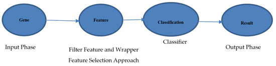
Figure 1.
Information gain (IG) flowchart.
3.1. Entropy and Information Gain (IG) for Gene Selection
Entropy is the basic concept used in information theory to compute the homogeneity of features; for example, when samples are fully homogeneous, they have an entropy equal to zero, whereas equally divided samples have an entropy value of one [20]. For a dataset with a high feature dimensionality and a small sample size, classification of the data is very difficult. Among the thousands of gene expression attributes that are usually investigated, only very few are relevant to a particular disease. Therefore, only the relevant features should be retained [13]. Proper investigation of the gene profiles will be helpful for selecting the genes that are most important for the classification process.
E(Z) = −D+log2 (D+) − D−log2 (D−) for a sample with negative and positive attributes.
The formula for entropy is as follows [21]:
where the are the a priori probabilities of categorical variable Z and is an index indicating a particular category in the classification system.
Consider the special case of two classification problems (where V is the number of classes).
Let j be a gene that may have n possible values (j1, j2, …, jn). The entropy will be as follows:
where is the conditional probability of variable K when attribute J is constant, calculated over all attributes and classes. The calculation of IG mainly depends on the entropy [22]. Based on the distribution of the attributes in the dataset, the entropy is calculated for all attributes in the dataset. The data are then separated into groups of attributes. The entropy is calculated for each group separately, and the entropy values for all groups are combined to obtain the total entropy. The entropy based on individual groups of data is then subtracted from the entropy based on the entire data distribution [23]:
when gene J and category K are not related, , whereas if they are related, then , leading to IG(J) > 0. There is a direct relationship between a larger difference between J and K and a stronger correlation between J and K. A feature with a larger IG value is more important for classification. Therefore, genes with greater IG values are first chosen from among the original high-dimensional genes to be used as the basis for further gene selection [24].
The IG flowchart shown in Figure 2 describes the steps of the IG algorithm. The input data set has a set of attributes W, and the required output is the selected subset Y of the original attributes W. First, the attributes to be considered for classification are initialized. Second, the entropy of all samples is computed for each class using Equation (1). Then, the conditional probability for each value of a single attribute is calculated and is used to calculate the conditional entropy for every attribute via Equation (2). The IG is computed using Equation (3) for all attributes. The resulting IG values are arranged in ascending order, and all values that are above a certain threshold value are selected.
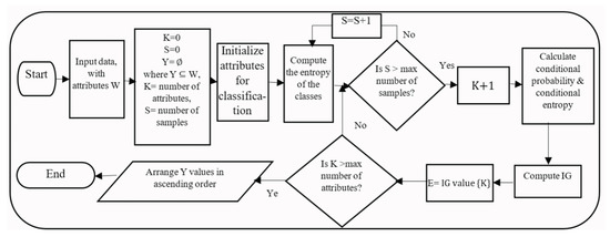
Figure 2.
IG flowchart.
3.2. Grey Wolf Optimization (GWO) for Feature Reduction
Wolves of the grey wolf (Canis lupus) species prefer to live in packs. On average, there are 5–12 members in one group. These animals live in groups governed by laws that maintain their hierarchical order, as shown in Figure 3 [25]. At the top of the hierarchy is the leader, called the alpha, who may be male or female. The alpha is responsible for most of the pack’s decisions, such as the places they hunt, the times at which they wake and sleep, and so on. All wolves in the pack follow the alpha [26]. The betas, who also may be male or female, constitute the second level in the hierarchy of grey wolves. They assist the alpha wolf in decision-making and coordinating other activities in the pack. A beta wolf is the most likely candidate to inherit the alpha’s position when the alpha dies or becomes too old to lead. The third level in the hierarchy of grey wolves consists of wolves called subordinates (or deltas). Deltas follow the alpha and beta wolves, and the others follow the deltas. The deltas of the pack are divided into several categories, each of which is responsible for particular tasks.
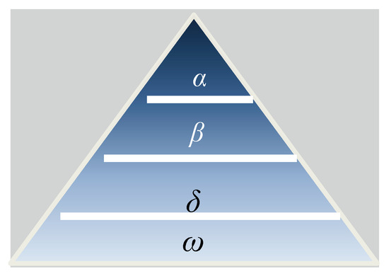
Figure 3.
Hierarchy of grey wolves (dominance decreases from the top down) [25].
The scout category is responsible for monitoring for threats to the pack [27]. The sentinel category is responsible for providing safety and protection for the pack. Elders are experienced wolves who are nominated to be future alphas or betas. Hunters assist the betas and alpha in hunting prey and providing food for the pack. Caretakers perform the caring tasks for wounded, ill, and weak wolves in the pack. All other wolves are omegas, who lie at the base of the hierarchy; they are the scapegoats. The omega wolves are subordinate to all other wolves in the hierarchy. They are the last to be allowed to eat. However, this does not mean that they are insignificant in the pack; without the omegas, the pack might collapse due to in-fighting. Furthermore, all wolves vent their violent tendencies by means of the omegas. This helps to maintain the hierarchical structure of the pack. The omegas also sometimes act as babysitters. Thus, all pack members participate in the leadership hierarchy. In the GWO algorithm, three primary hunting steps are performed for the purpose of optimization: seeking, encircling and attacking prey [28].
The Mathematical Model of GWO
In the mathematical formulation of GWO, the alpha (α) represents the fittest solution, and the next best solutions are the beta and delta (β) and (δ) solutions. Other solutions are regarded as omega (ω) solutions. In the GWO algorithm, the leadership consists of alpha (α), beta (β) and delta (δ) wolves. The remaining omega (ω) wolves are followers [29]. A mathematical representation of encircling behaviour is given by the following equations [30]:
here, represents the current iteration, and are coefficient vectors, is the prey’s position vector and represents the grey wolf’s position vector. The and vectors are calculated as follows:
where the magnitude of decreases linearly from two to zero over multiple iterations and and are random vectors between [0,1].
The update parameter b controls the trade-off between exploitation and exploration. The parameter b is updated linearly from owt to zero as follows:
where MxIter is the overall number of iterations and i is the number of the current iteration.
The grey wolves wish to identify the prey’s location and encircle it. To this end, the alpha guides the pack in the hunt. However, the grey wolves have no idea of the area to be searched or the location of the prey. To represent this idea mathematically, we assume that the alpha represents the best solution available. The beta and delta wolves assist in inferring the location of the prey. For this purpose, we need to identify the three best values and update their positions to approach as close as possible to the optimal solution. The position update is performed in accordance with the following equations, and a flowchart of the GWO algorithm is shown in Figure 4 [31].
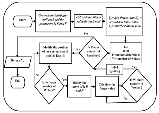
Figure 4.
GWO flowchart.
However, in the proposed system, the last Equation (15) is modified as shown in Equation (16) below:
3.3. Support Vector Machines (SVMs) for Classification
The SVM technique is one of the most popular techniques in machine learning. It depends on points of similarity, similar to KNN. However, it does not require the calculation of the distances between a new unseen point and all other data points at hand; rather, only the vectors that will influence the decision-making process are considered. The SVM approach is based on the idea of maximizing the margins between different classes. The greater the certainty of a classifier is, the larger are the margins it provides [32]. SVM classification is based on two key ideas:
- The notion of maximum margins and the concept of the kernel function;
- The area between a sample boundary and the nearest sample is called a margin. The support vectors represent these samples. In an SVM, the largest value is chosen to represent the margin.
For data with more than one dimension, an SVM classifier converts the data representation domain into a multi-dimensional domain and defines a hyperplane separating the data. The error (Err) and accuracy (Acc) of classification are used to evaluate the performance of an SVM classifier [16]:
where TruePo denotes the number of true positives, FalsePo denotes the number of false positives, TrueNe denotes the number of true negatives, and FalseNe denotes the number of false negatives.
Acc = (100 ∗ (TruePo + TrueNe))/(TrueNe + TruePo + FalseNe + FalsePo)
Err = (100 ∗ (FalsePo + FalseNe))/(TrueNe + TruePo+ FalseNe + FalsePo)
3.4. Proposed System Workflow
Our system is based on an IDSS. The system works as shown in Figure 5. First, the initial dataset, containing a set of attributes W, is entered into the system. (i) Calculate the IG value for each gene and then arrange the genes in descending order of their IG values. (ii) Select the attributes Y that have the highest IG values (higher than a predefined threshold) from among the attributes W. (iii) Initialize the grey wolf parameters (GWO), such as the population size, Yi, b, B, and E, and create the attribute set. (iv) Depending on the resulting wolves (selected feature subset), train an SVM classifier and evaluate its accuracy. (v) Calculate the fitness value of each search wolf (, , and ) using the SVM accuracy function. (vi) Update the positions of the current search agents using Equation (16). (vii) If the stopping condition (the maximum number of iterations) is not met, repeat steps (iv) and (v).
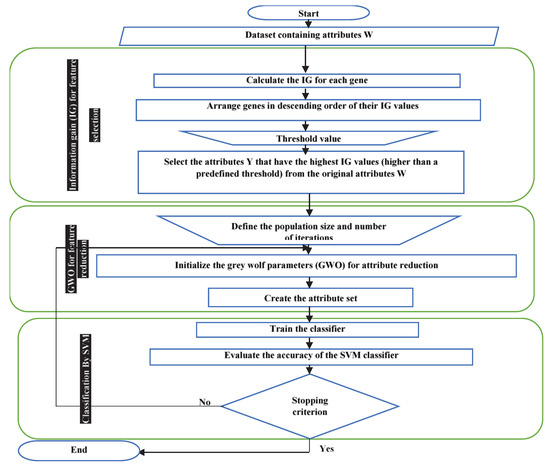
Figure 5.
Proposed system flowchart.
4. Performance Measures and Results
4.1. Microarray Datasets
The proposed system was evaluated using skewed cancer gene expression datasets downloaded from the Kent Ridge Bio-Medical Data Set website (http://datam.i2r.a-star.edu.sq/datasets/krbd/) [33]. The Kent Ridge Bio-Medical Data Set Repository is an online repository of high-dimensional biomedical datasets, including gene expression data, protein-profiling data and genomic sequence data that are related to classification. Each microarray dataset is in the form of a matrix that consists of M rows, corresponding to the samples, and N columns, corresponding to the genes. We used two sets of patient data to predict breast and colon cancer. Table 2 presents detailed information about the breast and colon cancer microarray datasets.
Table 2.
Descriptions of the datasets.
The breast cancer dataset contains 24,481 genes arranged in a matrix. The rows of the matrix represent the genes (features), while the columns represent the samples/instances (patients). This microarray dataset is divided into two matrices: a training matrix and a test matrix. Table 2 summarizes the details of the breast cancer microarray dataset. The training dataset contains prognosis results for 78 patients, 34 of whom are relapse cases and 44 of whom are non-relapse cases. The 34 relapse patients are those for whom distant metastases were observed within 5 years, while the remaining 44 non-relapse instances represent patients who remained cured of the disease for at least 5 years after preliminary diagnosis. The test matrix contains 12 relapse instances and seven non-relapse instances. For each test, two important criteria were utilized for observational assessment of the performance: the number of selected genes (features) and the classification accuracy [33].
Colon cancer, also called colorectal cancer, is a type of cancer caused by uncontrolled cell growth in the colon, rectum, or vermiform appendix. The two classes in the colon cancer dataset are somewhat different from those in the previous one. In the breast cancer dataset, all samples were collected from cancer patients, and the objective of the proposed classification system is to determine to which type of cancer a new sample belongs. By contrast, the colon cancer dataset contains data on 62 colon adenocarcinoma specimens taken from patients, 40 of which were real tumours and the other 22 of which were not tumours. Therefore, the objective of the classification system is to determine whether a new sample is a tumour. The gene expression data matrix contains the expression results for the 2000 genes with the highest minimal intensities across the 62 tissue samples. Accordingly, the entire gene expression data matrix has dimensions of 2000 * 62. The training data matrix here has dimensions of 2000 * 32, and the test data matrix has dimensions of 2000 * 30. Note that the genes are organized in the matrix in order of descending minimal intensity. This means that the expression values are not normalized with respect to the mean intensity in each experiment [15,33,34].
4.2. Accuracy Analysis
The number of true positives (TruePo) is the number of positive cases that are correctly detected. The number of true negatives (TrueNe) is the number of negative cases that are correctly detected. The number of false positives (FalsePo) is the number of negative cases that are diagnosed as positive. The number of false negatives (FalseNe) is the number of positive cases that are diagnosed as negative. The accuracy represents how close the predictions come to the actual values. A high accuracy and high precision indicate that the test procedure functions well with a meaningful hypothesis. The general equation for accuracy is as shown in Equation (17) [30].
4.3. Results Analysis
In this section, the proposed system is benchmarked on a gene expression profile dataset for breast and colon cancer that has been utilized by other researchers [10,13,14,15,33,35]. Three methodologies for classifying microarray datasets are considered. In the first, the SVM classifier is first applied without any feature selection, and then the wrapper feature selection approach based on the GWO algorithm is applied in combination with the same classifier on the same dataset; the results obtained in this way are presented in Table 3. In the second methodology, the filter feature selection approach based on the IG algorithm is applied in combination with the SVM classifier; the results are shown in Table 4. The third methodology involves a hybrid feature selection approach using both the IG algorithm and GWO in combination with SVM classification; this methodology achieves the best classification accuracy, as also shown in Table 4.
Table 3.
Classification accuracy achieved with the support vector machine (SVM) classifier alone and with SVM in combination with GWO using five-fold cross-validation.
Table 4.
Classification accuracy achieved with SVM classification in combination with IG feature selection with a threshold value of zero using five-fold cross-validation.
C#.net 2018 was used to implement the proposed system. The Weka tool suite version 3.8 was employed in C#.net to apply the IG filtering approach to each dataset for attribute selection. Then, the number of selected attributes was reduced by GWO, programmed in C#.net. Finally, the SVM classifier was called from Weka into C#.net to determine the final classification accuracy. The proposed system uses five-fold cross-validation [36].
Table 3 shows the results and parameter values for the first tested methodology. The breast cancer dataset contains 24,482 genes; when classification was performed on this dataset using the SVM classifier alone, the classification accuracy did not exceed 65%. When the data were first subjected to GWO with 35 wolves and 75 iterations, the classification accuracy increased to 71.795%, and the number of considered genes was reduced to 16,055; when the same original data were subjected to both IG filtering and GWO before SVM classification, the classification accuracy reached 88.46%, and the number of genes was reduced to 455, as shown in Table 4. Table 3 also shows the results and parameter settings for the colon cancer dataset. This dataset contains 2000 genes, and when classification was performed on this dataset using the SVM classifier alone, the classification accuracy did not exceed 63%. When the data were first subjected to GWO with 120 wolves and 160 iterations, the classification accuracy increased to 85.484%, and the number of considered genes was reduced to 999; when the same original data were subjected to both IG filtering and GWO before SVM classification, the classification accuracy reached 90.32%, and the number of genes was reduced to 70, as shown in Table 4.
Table 5 and Table 6 show the parameter settings and the results obtained with the proposed system with and without GWO, respectively, using five-fold cross-validation. The parameter settings are the same as those in Table 4 except that the IG threshold value is varied. As seen from Table 4 and Table 5, when the threshold value was changed to 0.17 or to 0.2 or more, the classification accuracy achieved was lower than the best result achieved with a threshold value of zero. However, although better accuracy results were achieved with no threshold IG value, using a threshold made it possible to reduce the number of features from 7129 to 32, thereby decreasing the time and memory consumption needed for the classification process.
Table 5.
Classification accuracy achieved with SVM classification in combination with IG feature selection with multiple IG thresholds using five-fold cross-validation.
Table 6.
Classification accuracy achieved with IG + GWO + SVM with multiple IG thresholds using five-fold cross-validation.
Table 7 summarizes the best results obtained when applying the proposed methodology to the two datasets (Breast and Colon). In Table 8, we review the classification accuracies of several different classifiers for comparison with the SVM classifier.
Table 7.
Best results with multiple IG threshold values.
Table 8.
Accuracy comparison of several different classifiers.
Table 9 and Table 10 show the differences between the classification accuracies of different methodologies based on hybrid feature selection approaches (filter and wrapper approaches) when applied to colon and breast cancer data. As shown, the best results achieved with the proposed methodology are 94.87% (Breast) and 95.935% (Colon). The proposed method applied feature selection and reduction; this strategy improves the performance of our method. The other authors used only feature selection or reduction techniques. Overall, we observed that the feature selection and reduction method which selects features by IG and GWO estimated on different bootstrap samples increased the stability of classification. Regarding the choice of method to train a classifier once features are selected and reduced, we observed that the best accuracy was achieved by our method. An advantage of our SVM classifier is that it does not require any parameter tuning, making the computations fast and less prone to overfitting. A comparison of the experimental results reveals that the proposed system offers improved sample classification accuracy. These experimental results show that the proposed strategy is able to improve the stability of the feature selection results as well as the sample classification accuracy.
Table 9.
Classification accuracy of the proposed methodology vs. other methodologies on Breast.
Table 10.
Classification accuracy of the proposed methodology vs. other methodologies on Colon.
Random sampling [37,38] is essentially biased compared to amenable analytical treatment and can lead to different results. The result depends on several factors, such as the sampling method and the amount of data missing. One of the disadvantages of our method is considered when using missing data and also when the data was imbalanced. Unsupervised learning is considered to be a good option to counter the problem of unlabelled data.
5. Conclusions and Future Works
In this research, an enhanced IDSS is proposed based on IG feature selection, the GWO algorithm and SVM classification. The proposed system employs the IG method for initial feature selection, while GWO is used to reduce the number of selected features to enable more accurate sample classification by the SVM. Two microarray datasets are used as benchmarks to evaluate the proposed methodology. The experimental results indicate that the proposed methodology is able to enhance the stability of the classification accuracy as well as the feature selection. The best results are obtained when combining the IG approach with both the GWO and SVM algorithms; the classification accuracy reaches 94.87% for breast cancer data and 95.935% for colon cancer data. In future work, additional classifiers, such as decision tree, neural network, and k-nearest neighbour should be added to the system. In addition, there is a possibility of testing the system on other benchmarks, especially binary-class datasets and test the reliability of diagnosis after repeated sampling of tissue from the same patient.
Author Contributions
All authors contributed equally to this work. All authors have read and agree to the published version of the manuscript.
Funding
The authors would like to thank NVIDIA Corporation with the donation of the Titan X GPU used in this research.
Conflicts of Interest
The author declares no conflict of interest.
References
- Walker, D.; Bendel, A.; Stiller, C.; Indelicato, D.; Smith, S.; Murray, M.; Bleyer, A. Central Nervous System Tumors. In Pediatric Oncology; Springer: Cham, Switzerland, 2017; pp. 335–381. ISBN 978-3-319-33677-0. [Google Scholar]
- Cancer.net. American Society of Clinical Oncology (ASCO). Available online: https://www.cancer.net/cancer-types/central-nervous-system-childhood/view-all (accessed on 1 January 2020).
- Janghel, R.R.; Shukla, A.; Tiwari, R.; Kala, R. Intelligent Decision Support System for Breast Cancer. In Proceedings of the Advances in Swarm Intelligence, Beijing, China, 12–15 June 2010; Tan, Y., Shi, Y., Tan, K.C., Eds.; Springer: Berlin/Heidelberg, Germany, 2010; pp. 351–358. [Google Scholar]
- Siegel, R.L.; Miller, K.D.; Jemal, A. Cancer statistics, 2020. CA A Cancer J. Clin. 2020, 70, 7–30. [Google Scholar] [CrossRef]
- Al-Badareen, A.B.; Selamat, M.H.; Samat, M.H.; Nazira, Y.; Akkanat, O. A Review on Clinical Decision Support Systems in Healthcare. Available online: /paper/A-review-on-clinical-decision-support-systems-in-Al-Badareen-Selamat/cb1e1c668f6e0def2f893b3669f5e9766033f258 (accessed on 1 January 2020).
- Doi, K. Computer-Aided Diagnosis in Medical Imaging: Historical Review, Current Status and Future Potential. Comput. Med. Imaging Graph. 2007, 31, 198–211. [Google Scholar] [CrossRef]
- Ahsen, M.E.; Boren, T.P.; Singh, N.K.; Misganaw, B.; Mutch, D.G.; Moore, K.N.; Backes, F.J.; McCourt, C.K.; Lea, J.S.; Miller, D.S.; et al. Sparse feature selection for classification and prediction of metastasis in endometrial cancer. BMC Genomics 2017, 18, 233. [Google Scholar] [CrossRef]
- Berg, W.A.; Gutierrez, L.; NessAiver, M.S.; Carter, W.B.; Bhargavan, M.; Lewis, R.S.; Ioffe, O.B. Diagnostic Accuracy of Mammography, Clinical Examination, US, and MR Imaging in Preoperative Assessment of Breast Cancer. Radiology 2004, 233, 830–849. [Google Scholar] [CrossRef]
- Elyasigomari, V.; Lee, D.A.; Screen, H.R.C.; Shaheed, M.H. Development of a two-stage gene selection method that incorporates a novel hybrid approach using the cuckoo optimization algorithm and harmony search for cancer classification. J. Biomed. Inform. 2017, 67, 11–20. [Google Scholar] [CrossRef]
- Salem, H.; Attiya, G.; El-Fishawy, N. Classification of human cancer diseases by gene expression profiles. Appl. Soft Comput. 2017, 50, 124–134. [Google Scholar] [CrossRef]
- Salem, H.; Attiya, G.; El-Fishawy, N. Early diagnosis of breast cancer by gene expression profiles. Pattern Anal. Appl. 2017, 20, 567–578. [Google Scholar] [CrossRef]
- Bennet, J.; Ganaprakasam, C.; Kumar, N. A hybrid approach for gene selection and classification using support vector machine. Int. Arab J. Inf. Technol. 2015. [Google Scholar]
- Yeh, J.-Y.; Wu, T.-S.; Wu, M.-C.; Chang, D.-M. Applying Data Mining Techniques for Cancer Classification from Gene Expression Data. In Proceedings of the 2007 International Conference on Convergence Information Technology (ICCIT 2007), Gyeongju, South Korea, 21–23 November 2007; pp. 703–708. [Google Scholar] [CrossRef]
- Bolón-Canedo, V.; Sánchez-Maroño, N.; Alonso-Betanzos, A. An ensemble of filters and classifiers for microarray data classification. Pattern Recognit. 2012, 45, 531–539. [Google Scholar]
- Gunavathi, C.; Premalatha, K. Performance Analysis of Genetic Algorithm with kNN and SVM for Feature Selection in Tumor Classification; 2014. [Google Scholar]
- Bouazza, S.H.; Hamdi, N.; Zeroual, A.; Auhmani, K. Gene-expression-based cancer classification through feature selection with KNN and SVM classifiers. In Proceedings of the 2015 Intelligent Systems and Computer Vision (ISCV), Fez, Morocco, 25–26 March 2015; pp. 1–6. [Google Scholar]
- Emary, E.; Zawbaa, H.M.; Grosan, C.; Hassenian, A.E. Feature Subset Selection Approach by Gray-Wolf Optimization. In Proceedings of the Afro-European Conference for Industrial Advancement, Villejuif (Paris-sud), France, 9–11 September 2015; Abraham, A., Krömer, P., Snasel, V., Eds.; Springer International Publishing: Cham, Switzerland, 2015; pp. 1–13. [Google Scholar]
- Paul, A.; Sil, J.; Mukhopadhyay, C.D. Gene selection for designing optimal fuzzy rule base classifier by estimating missing value. Appl. Soft Comput. 2017, 55, 276–288. [Google Scholar] [CrossRef]
- Hira, Z.M.; Gillies, D.F. A Review of Feature Selection and Feature Extraction Methods Applied on Microarray Data. Adv. Bioinform. 2015, 2015, 198363. [Google Scholar] [CrossRef]
- Baez, J.C.; Fritz, T.; Leinster, T. A Characterization of Entropy in Terms of Information Loss. Entropy 2011, 13, 1945–1957. [Google Scholar] [CrossRef]
- Chen, L.; Wu, K.; Li, Y. A Load Balancing Algorithm Based on Maximum Entropy Methods in Homogeneous Clusters. Entropy 2014, 16, 5677–5697. [Google Scholar] [CrossRef]
- Mwadulo, M. A Review on Feature Selection Methods For Classification Tasks. Int. J. Comput. Appl. Technol. Res. 2016, 5, 395–402. [Google Scholar]
- Okun, O. Feature Selection and Ensemble Methods for Bioinformatics: Algorithmic Classification and Implementations; 2011. [Google Scholar]
- Bramer, M. Principles of Data Mining; Undergraduate Topics in Computer Science; Springer: London, UK, 2007; ISBN 978-1-84628-766-4. [Google Scholar]
- Grey Wolf Optimizer. Adv. Eng. Softw. 2014, 69, 46–61. [CrossRef]
- Mech, L.D. Alpha Status, Dominance, and Division of Labor in Wolf Packs; 1999. [Google Scholar]
- Kumar, D.P.S.; Sathyadevi, G. Decision Support System for Medical Diagnosis Using Data Mining; 2011. [Google Scholar]
- Muro, C.; Escobedo, R.; Spector, L.; Coppinger, R.P. Wolf-pack (Canis lupus) hunting strategies emerge from simple rules in computational simulations. Behav. Process. 2011, 88, 192–197. [Google Scholar] [CrossRef]
- Pomeroy, S.L.; Tamayo, P.; Gaasenbeek, M.; Sturla, L.M.; Angelo, M.; McLaughlin, M.E.; Kim, J.Y.H.; Goumnerova, L.C.; Black, P.M.; Lau, C.; et al. Prediction of central nervous system embryonal tumour outcome based on gene expression. Nature 2002, 415, 436–442. [Google Scholar] [CrossRef]
- Song, X.; Tang, L.; Zhao, S.; Zhang, X.; Li, L.; Huang, J.; Cai, W. Grey Wolf Optimizer for parameter estimation in surface waves. Soil Dyn. Earthq. Eng. 2015, 75, 147–157. [Google Scholar] [CrossRef]
- Emary, E.; Zawbaa, H.M.; Hassanien, A.E. Binary grey wolf optimization approaches for feature selection. Neurocomputing 2016, 172, 371–381. [Google Scholar] [CrossRef]
- Marsland, S. Machine Learning: An Algorithmic Perspective, 2nd ed.; Chapman & Hall/CRC: Boca Raton, FL, USA, 2014; ISBN 1-4665-8328-2. [Google Scholar]
- Alonso-González, C.J.; Moro-Sancho, Q.I.; Simon-Hurtado, A.; Varela-Arrabal, R. Microarray gene expression classification with few genes: Criteria to combine attribute selection and classification methods. Expert Syst. Appl. 2012, 39, 7270–7280. [Google Scholar]
- Pyingkodi, M.; Thangarajan, R. Informative Gene Selection for Cancer Classification with Microarray Data Using a Metaheuristic Framework. Asian Pac. J. Cancer Prev. 2018, 19, 561–564. [Google Scholar] [PubMed]
- Cho, S.-B.; Won, H.-H. Machine Learning in DNA Microarray Analysis for Cancer Classification. In First Asia-Pacific Bioinformatics Conference on Bioinformatics 2003—Volume 19; Australian Computer Society, Inc.: Adelaide, Australia, 2003; pp. 189–198. [Google Scholar]
- Isaksson, A.; Wallman, M.; Göransson, H.; Gustafsson, M.G. Cross-validation and bootstrapping are unreliable in small sample classification. Pattern Recognit. Lett. 2008, 29, 1960–1965. [Google Scholar] [CrossRef]
- Moteghaed, N.Y.; Maghooli, K.; Garshasbi, M. Improving Classification of Cancer and Mining Biomarkers from Gene Expression Profiles Using Hybrid Optimization Algorithms and Fuzzy Support Vector Machine. J. Med. Signals Sens. 2018, 8, 1–11. [Google Scholar] [PubMed]
- Shang, Y. Subgraph Robustness of Complex Networks Under Attacks. IEEE Trans. Syst. Man Cybern. Syst. 2019, 49, 821–832. [Google Scholar] [CrossRef]
© 2020 by the authors. Licensee MDPI, Basel, Switzerland. This article is an open access article distributed under the terms and conditions of the Creative Commons Attribution (CC BY) license (http://creativecommons.org/licenses/by/4.0/).