Failure Prediction Model Using Iterative Feature Selection for Industrial Internet of Things


1
Smart Computing Laboratory, Hallym University, 1 Hallymdaehak-gil, Chuncheon, Gangwon-do 24252, Korea
2
School of Software, Hallym University, 1 Hallymdaehak-gil, Chuncheon, Gangwon-do 24252, Korea
*
Author to whom correspondence should be addressed.
Symmetry 2020, 12(3), 454; https://doi.org/10.3390/sym12030454
Submission received: 30 January 2020
/
Revised: 5 March 2020
/
Accepted: 8 March 2020
/
Published: 12 March 2020
(This article belongs to the Special Issue Selected Papers from IIKII 2019 conferences in Symmetry)
Abstract
:This paper presents a failure prediction model using iterative feature selection, which aims to accurately predict the failure occurrences in industrial Internet of Things (IIoT) environments. In general, vast amounts of data are collected from various sensors in an IIoT environment, and they are analyzed to prevent failures by predicting their occurrence. However, the collected data may include data irrelevant to failures and thereby decrease the prediction accuracy. To address this problem, we propose a failure prediction model using iterative feature selection. To build the model, the relevancy between each feature (i.e., each sensor) and the failure was analyzed using the random forest algorithm, to obtain the importance of the features. Then, feature selection and model building were conducted iteratively. In each iteration, a new feature was selected considering the importance and added to the selected feature set. The failure prediction model was built for each iteration via the support vector machine (SVM). Finally, the failure prediction model having the highest prediction accuracy was selected. The experimental implementation was conducted using open-source R. The results showed that the proposed failure prediction model achieved high prediction accuracy.
1. Introduction
Recently, the industrial Internet of Things (IIoT) has been widely adopted by various companies, as it provides connectivity and analysis capabilities, which are the key technologies for advanced manufacturing [1,2,3,4]. In IIoT, a large number of sensors are used to periodically detect changes in machine health, manufacturing process, industrial environment, etc. [5,6,7,8,9,10]. Hence, a huge amount of data is collected from the sensors used in IIoT. In general, the collected data are analyzed to provide useful information for productivity improvement [11]. In particular, failure prediction through data analysis is considered one of the most important issues in IIoT [12]. The failure, such as execution error, long delay, and defective product, leads to a fatal system malfunction and huge maintenance cost, resulting in productivity degradation of enterprises in industrial fields [13]. Therefore, many enterprises have endeavored to predict when and why failures occur for improving their capabilities of failure prevention and recovery, also known as resilience capacity [14]. Especially, the accuracy of failure prediction is an important factor that determines the resilience capacity of enterprises; thus, its improvement is crucial in the IIoT.
To predict failures, we need to build a failure prediction model that determines whether or not a failure occurs [15,16,17]. In order to build such a failure prediction model, most of the existing studies have used machine learning techniques. Abu-Samah et al. built the failure prediction model on the basis of a Bayesian network, and Kwon and Kim (i.e., our previous work) used the nearest centroid classification to predict machine failures [18,19]. The results of both the studies showed that the built failure prediction model achieved approximately 80% prediction accuracy. However, they did not conduct the feature selection. In other words, they used all the data in the dataset when building the model. Accordingly, in a real IIoT context where a very large number of sensors are used, the prediction accuracy might be significantly degraded because of the impact of the data irrelevant to the failures.
Therefore, feature selection has been considered one of the most important steps in building a failure prediction model. There have been many studies to build the failure prediction model using feature selection, most of which have selected features considering the importance of each feature [20,21,22]. Moldovan et al. built a failure prediction model using the selected features to improve prediction accuracy and performed feature selection using three algorithms (i.e., random forest, regression analysis, and orthogonal linear transformation) to compare the prediction accuracy of each for the comparative study [20]. Mahadevan and Shah used a support vector machine recursive feature elimination (SVM-RFE) algorithm to rank the features by their importance [21]. The SVM-RFE algorithm was used to compute the norm of the weights of each feature (i.e., the importance of each feature). For feature selection, the authors determined a threshold value specified by the limit of the number of selected features, and then selected the features considering their importance until the number of selected features reached the threshold. The selected features were used for failure detection and diagnosis. Hasan et al. focused on a two-step approach of random forest based-feature selection, which consists of the feature importance measurement and feature selection [22]. In the first step, the importance of each feature was measured using average permutation importance (APIM) score. APIM score is obtained by calculating the mean decreases in the forest’s classification accuracy when a specific feature is not available. In the second step, the features with an APIM score greater than a threshold were selected. However, in the existing feature selection methods, the optimal prediction accuracy cannot be obtained because the number of selected features is fixed or all the features in which the importance is greater than a predefined threshold are selected. Specifically, the number of selected features might be too large to obtain optimal prediction accuracy or vice versa.
In this paper, we propose a novel failure prediction model using iterative feature selection, which aims to accurately predict the occurrence of failures. To build the model, the collected data are processed and analyzed using the following steps: (1) preprocessing, (2) importance measurement, (3) feature selection, (4) model building, and (5) model selection. The preprocessing step includes feature elimination, missing data imputation, normalization, and data division. In the importance measurement step, to measure the importance of each feature, the relevancy between each feature and the failure is analyzed using the random forest algorithm [23,24,25,26]. Then, the feature selection and model building steps are conducted iteratively. In particular, in the feature selection step, a new feature is selected considering its importance in each iteration and is added to the selected feature set. In the model building step, the failure prediction model is built via the SVM on the basis of the selected feature set updated in each iteration [27,28,29,30]. Finally, one of the failure prediction models is selected considering the prediction accuracy in the model selection step. To evaluate the performance of the proposed model, we conducted an experimental implementation using open-source R. We used the semiconductor manufacturing (SECOM) dataset provided by the University of California Irvine (UCI) repository [31]. The results showed that the proposed failure prediction model achieved high prediction accuracy.
2. Failure Prediction Model Using Iterative Feature Selection
In this section, we present the design of the failure prediction model using iterative feature selection in detail. It is assumed that sensors with unique identification (ID) employed in an IIoT environment periodically generate data, and the data is collected by a data analysis server. In this paper, the sensor device is represented as a feature, and its ID is represented by a feature index. The data analysis server collects data from sensor devices and builds and evaluates the failure prediction model. The data is represented in the form of a matrix format (i.e., dataset) in which each column and row means the feature and data collection time, respectively.
We built the failure prediction model on the basis of the features selected to maximize the prediction accuracy. To this end, feature selection was iteratively conducted, and multiple failure prediction models were built on the basis of the features selected in each iteration. Then, the failure prediction model with the highest prediction accuracy was selected. To build the failure prediction model, we considered five steps, namely preprocessing, importance measurement, feature selection, model building, and model selection. In this section, each step for building the failure prediction model is described in detail.
Figure 1 shows the overall procedure for building the failure prediction model. In the figure, the white square indicates each step, and the grey square indicates the input or output of each step. In the preprocessing step, feature elimination, missing data imputation, normalization, and data division are sequentially conducted. To eliminate invalid features from the input dataset (i.e., collected data), the not applicable (NA) data of each feature are searched, and the variance of each feature is calculated. If the ratio of the NA data of a specific feature is greater than the predefined validity factor determined in the range [0, 1], the corresponding feature is eliminated from the input dataset. Moreover, if the variance of a certain feature is close to zero, the corresponding feature is eliminated from the input dataset. This is because the closer the variance of a certain feature is to zero, the more similar is the value of all the data. In particular, if the variance of a certain feature is zero, all the data of this feature have the same value, which means that the feature is meaningless for the data analysis. To replace the remaining missing data with the appropriate data, an average of the non-missing data of each feature is calculated and imputed. Then, normalization is conducted to match the data scale of each feature. To this end, the standard score is used, which calculates the normalized data of each feature according to Equation (1):
where is the -th normalized data of the feature, is the -th data of the feature, is the average of the feature, and is the standard deviation of the feature [32]. The and values are calculated using Equations (2) and (3), respectively [33].
where is the amount of data of the feature. Finally, the normalized dataset is divided into training and test datasets, which are used to build the failure prediction model and to evaluate the performance of the prediction model, respectively.
To measure the importance of each feature, the training dataset (i.e., a part of the preprocessed dataset) is analyzed using the random forest algorithm, which is one of the machine learning techniques for importance measurement. In particular, via the random forest, multiple decision trees are built, and the relevancy between each feature and the failure is analyzed considering the built decision trees comprehensively. In the random forest, multiple subsets of the training dataset are created to build each decision tree differently. Note that each subset consists of different data and features. For this, n data (i.e., n rows) and mtry features (i.e., mtry columns) are randomly selected from the training dataset. This operation repeats until the number of created subsets reaches the number of decision trees predefined as ntree. Then, each decision tree is built separately using one of the created subsets. After building ntree decision trees, the importance of each feature is measured through the mean decrease Gini, which indicates the extent to which each feature affects the correct prediction results. More specifically, in each decision tree, the sum of the difference for Gini impurities between the parent nodes using a particular feature and their child nodes is calculated. Then, the average of the results of all the decision trees is calculated. Note that the decision tree consists of multiple nodes that make decisions using the threshold of a specific feature. In addition, each node has a Gini impurity that is a measurement of the likelihood of an incorrect decision.
Then, the feature selection and model building steps are conducted iteratively. Algorithm 1 shows the overall operation of both the steps. In the algorithm, the set of the importance of features and the set of features are represented by Equations (4) and (5), respectively.
where is the number of features and is the importance of the -th feature. The index of each element in and (i.e., index of each importance and feature) denotes the sequence number of each feature. At the beginning of the algorithm, the variables are initialized: the selected feature at the -th iteration (), the prediction accuracy for the built model at the -th iteration (), and the iteration counter (). Then, the feature selection and model building steps are repeated until the importance of a newly selected feature is smaller than the importance threshold. In the algorithm, the maximum number of iterations () is equal to the number of features whose importance is greater than the importance threshold. Therefore, the iteration terminates when reaches . In each iteration, the feature selection step selects a new feature with the highest importance and adds it to the selected feature set represented by Equation (6).
Consequently, the number of features included in is incremented by one as the number of iteration increases. Once is updated, the model building step builds the failure prediction model through SVM on the basis of . Then, it evaluates the prediction accuracy to update the prediction accuracy set that is expressed by Equation (7).
Note that the index of each element in and (i.e., index of each selected feature and prediction accuracy) refers to the number of iterations. In the algorithm, modelBuildEvalFunction() is a function to build and evaluate the prediction model. It derives the prediction accuracy by taking he prediction model. It derives the prediction accuracy by taking as the input. For example, if (i.e., the third iteration) and the selected feature set is equal to the (i.e., , , and ), modelBuildEvalFunction() first builds the failure prediction model using the training data of the features in the . Then, it derives by evaluating the built model using the test data of the features and updates the prediction accuracy set from to . In the example, the number of elements in increases from two to three. When reaches , the operation is terminated. The outputs of this operation are shown in Equations (8) and (9).
| Algorithm 1: Operation of feature selection and model building steps. | |
| 1: | INITIALIZE to NULL, to 0, and to 0 //Initialize variables |
| 2: | REPEAT //Start iteration |
| 3: | /* ========== Feature Selection Step ========== */ |
| 4: | ← //Find the highest importance from |
| 5: | FOR each feature index, , |
| 6: | IF == //Find feature index with the highest importance |
| 7: | ← //Select a new feature |
| 8: | ← 0 //Remove the selected feature from and |
| 9: | ENDIF |
| 10: | ENDFOR |
| 11: | ← //Update the selected feature set |
| 12: | /* ========== Model Building Step ========== */ |
| 13: | ← modelBuildEvalFunction() //Build and evaluate model |
| 14: | ← //Update the prediction accuracy set |
| 15: | ← //Increment iteration counter by one |
| 16: | UNTIL //Terminate iteration if condition becomes TRUE |
| 17: | RETURN and //Return selected feature set and prediction accuracy set |
The model selection step selects the failure prediction model having the highest prediction accuracy, referring to and . In particular, this step first searches for the highest prediction accuracy in by using , where is the function that searches the element having the maximum value in a given set. Then, it derives the index of from . For this, each element in is compared with , and the index of the element that is equal to is derived from . Finally, a failure prediction model is selected, taking into account the index of and . More specifically, the elements (i.e., selected features) in which the index is less than or equal to the index of are extracted from . Then, one of the failure prediction models built in the model building step is selected by comparing the features used in the model building step and the extracted features from .
3. Implementation and Performance Evaluation
An experimental implementation was conducted to verify the feasibility of the proposed failure prediction model by using the open-source R version 3.4.3. For this, the SECOM dataset provided by the UCI repository was used. This dataset consists of 1567 data elements and 591 features, and the data were collected from a semiconductor manufacturing process by monitoring the sensors and the process measurement point. The data of 590 features were measured from different sensors, and the data of the remaining feature were the results of the house line test represented by Pass and Fail.
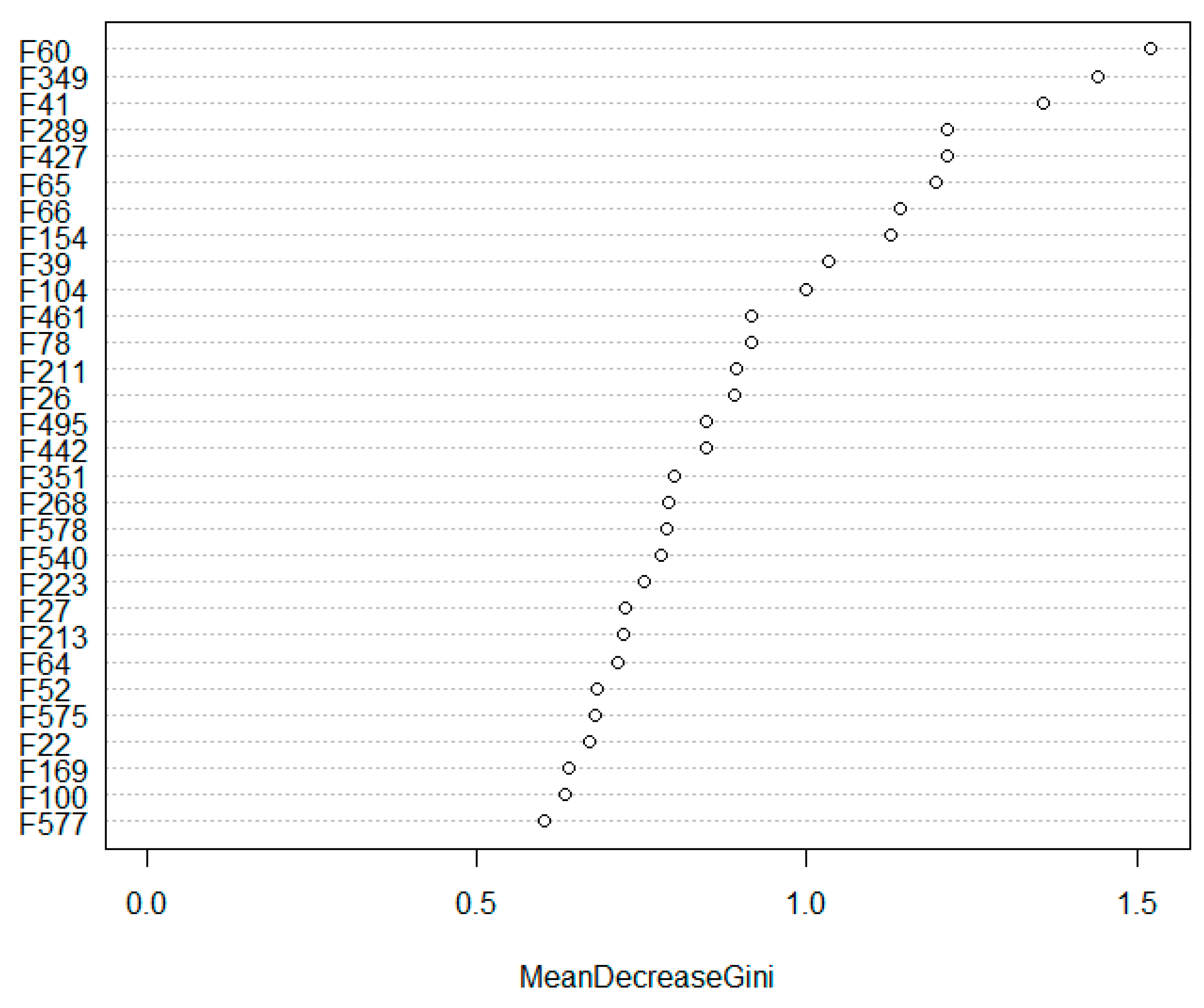
For feature elimination, we set the validity factor to 0.1, which was empirically determined to maximize the prediction accuracy. Thus, features with more than 10% NA data and features having zero variance were eliminated from the dataset. Through feature elimination, the number of features reduced from 591 to 393. The ratio of the training dataset and the test dataset was set to 7:3. To measure the importance of each feature, we used the randomForest and caret packages. We set n, mtry, and ntree to 1000, 19, and 500, respectively. Through this setting, 500 decision trees were built using the randomly created 1000 × 19 matrix. The importance of each feature was measured through the mean decrease Gini. Figure 2 shows the importance of the top 30 features. The x-axis and the y-axis denote the mean decrease Gini and the feature, respectively. In the figure, F60 has the highest mean decrease Gini (i.e., 1.52) among all the features.
For iterative feature selection, we set the importance threshold to 0.7, which was chosen in the range of [0.1, 1], taking into account the feature selection results of the existing research for the comparative study. Therefore, was determined as 24. This implied that the number of iterations was 24. The training dataset contained 70 fails and 1038 passes. This imbalance of the training dataset made it difficult for the failure prediction model to predict a fail case. To address this problem, the sampling was conducted before building the failure prediction model. In particular, some of the pass data were removed to have less effect on the model building. With the results of feature selection and the sampled training dataset, the failure prediction model was built using the SVM. To this end, we used the e1071 package in R. Table 1 lists the obtained and . In the table, is 0.72, and its index is 7. As a result, the failure prediction model that was built using eight features (i.e., F60, F349, F41, F289, F427, F65, F66, and F154) was selected.
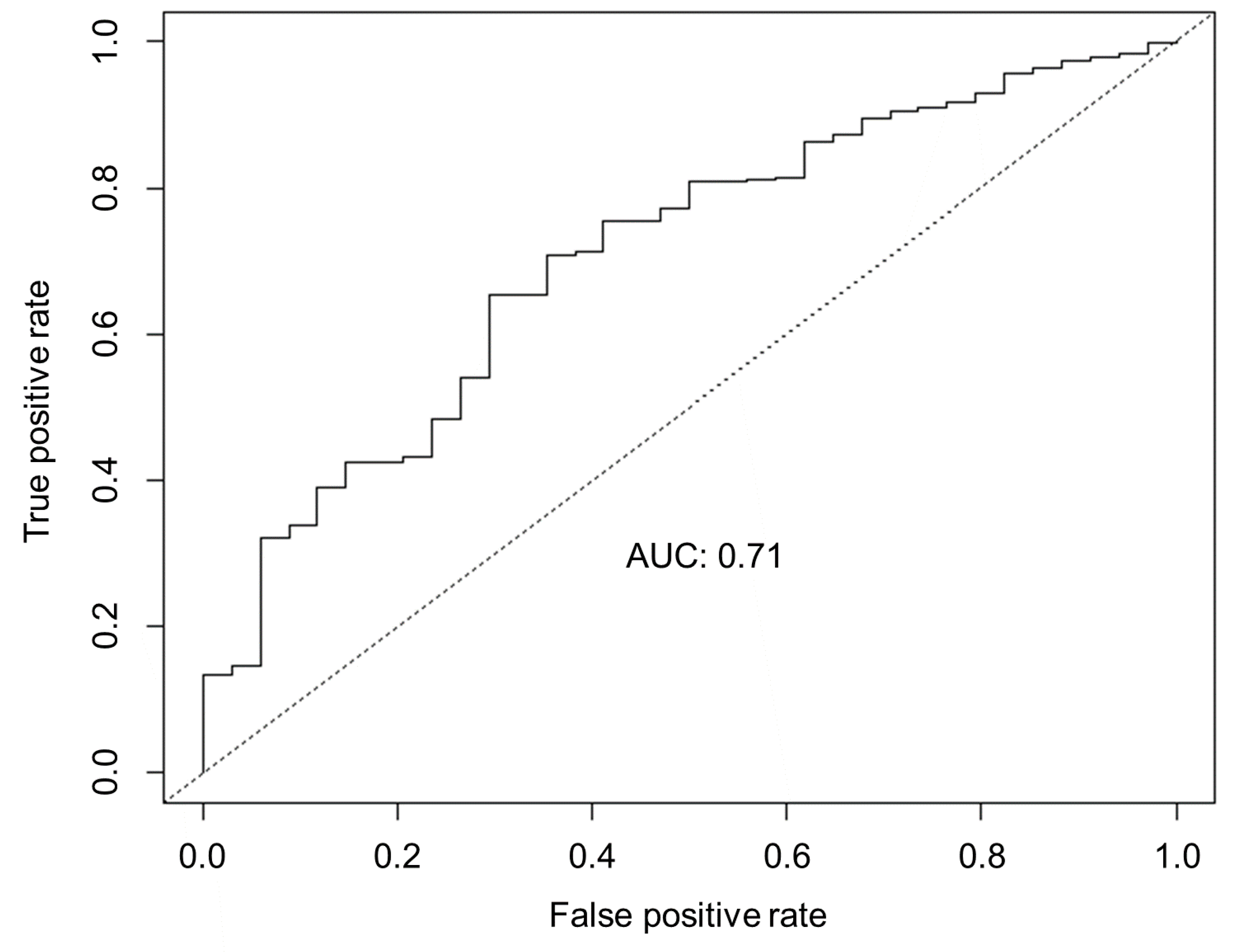
For the performance evaluation, the prediction accuracy of the proposed model was compared to that of the existing models. We considered three existing models, which were built on the basis of a fixed number of features (i.e., 12 and 24 features) and all the features, respectively. Figure 3, Figure 4, Figure 5 and Figure 6 show the receiver operating characteristic (ROC) curve for the three failure prediction models that used different numbers of features. The ROC curve is a performance measure of the prediction model and presents the relationship between the true positive rate (TPR) and the false positive rate (FPR) [34]. The TPR and FPR values were calculated using Equations (10) and (11), respectively.
where , , , and are the true positive, false negative, false positive, and true negative, respectively. With the ROC curve, the area under the curve (AUC) was used to evaluate the prediction accuracy of the model. In particular, the greater the AUC was, the higher was the prediction accuracy. In Figure 3, the failure prediction model that was built on the basis of iterative feature selection has the greatest AUC among the considered models. This was because the model was iteratively built using a different number of features; one of the models, i.e., the one with the highest prediction accuracy, was selected. As shown in Figure 4 and Figure 5, if a fixed number of features are used for building the model, the prediction accuracy might be relatively degraded. The reason was that irrelevant features made it difficult to build accurate prediction models. If more features irrelevant to the failure were used to build the model, the prediction accuracy of the model decreased. Therefore, in the case that all the features in the dataset were used as shown in Figure 6, the AUC decreased significantly. Quantitatively, the proposed model achieved 14.3% and 22.0% higher AUC than in the fixed number of features and the all features cases, respectively.
4. Conclusions
In this paper, we proposed a failure prediction model using iterative feature selection with the aim of predicting the failure occurrences. The procedure for building the failure prediction model consisted of the following five steps: (1) preprocessing, (2) importance measurement, (3) feature selection, (4) model building, and (5) model selection. In the first step, feature elimination, missing data imputation, normalization, and data division are sequentially conducted. The importance measurement step is to measure the importance of each feature by using the random forest. The third and the fourth steps were iteratively performed to build the failure prediction models using the various selected feature sets and to obtain the prediction accuracy of the built models. In the last step, the failure prediction model with the highest prediction accuracy was selected. The experimental implementation was conducted to evaluate the performance of the proposed model using the open-source R and the SECOM dataset given by the UCI repository. Through the experimental implementation, we obtained the importance of features representing the relevancy between each feature and failure. Moreover, we obtained the selected feature set and prediction accuracy set, each of which contains twenty-four features and prediction accuracy measurements. In the experiments, the proposed failure prediction model was built with eight features, and we compared the prediction accuracy of the proposed model with that of the failure prediction model built based on 12 features, 24 features, and all features. The results showed that the proposed model achieved 1.4%, 14.3%, and 22.0% higher AUC than that of other models. Comprehensively, the contributions of this paper are as follows. (1) We presented and discussed the problems of the existing failure prediction models for IIoT. (2) Through the importance measurement and iterative feature selection, we derived the feature index and the number of features that maximize the prediction accuracy of the failure prediction model. (3) We verified the feasibility of our work by conducting open-source-based implementation and extensive experiments. In our work, the proposed failure prediction model was implemented using only a limited dataset. Therefore, future work involves performing additional experiments with extended datasets to assess whether the proposed model is useful for various IIoT applications.
Author Contributions
E.-J.K. conceived and designed the failure prediction model; J.-H.K. performed the implementation and experiment; E.-J.K. interpreted and analyzed the data; J.-H.K. and E.-J.K. wrote the paper; E.-J.K. guided the research direction and supervised the entire research process. All authors have read and agree to the published version of the manuscript.
Funding
This research was supported by Hallym University Research Fund, 2019 (HRF-201911-010).
Conflicts of Interest
The authors declare no conflict of interest.
References
- Cheng, J.; Chen, W.; Tao, F.; Lin, C.-L. Industrial IoT in 5G environment towards smart manufacturing. J. Ind. Inf. Integr. 2018, 10, 10–19. [Google Scholar] [CrossRef]
- Kaur, K.; Garg, S.; Aujla, G.S.; Kumar, N.; Rodrigues, J.J.; Guizani, M. Edge Computing in the Industrial Internet of Things Environment: Software-Defined-Networks-Based Edge-Cloud Interplay. IEEE Commun. Mag. 2018, 56, 44–51. [Google Scholar] [CrossRef]
- Zhu, C.; Rodrigues, J.J.; Leung, V.C.; Shu, L.; Yang, L.T. Trust-based Communication for the Industrial Internet of Things. IEEE Commun. Mag. 2018, 56, 16–22. [Google Scholar] [CrossRef]
- Talavera, J.M.; Tobon, L.E.; Gomez, J.A.; Culman, M.A.; Aranda, J.M.; Parra, D.T.; Quiroz, L.A.; Hoyos, A.; Garreta, L.E. Review of IoT applications in agro-industrial and environmental fields. Comput. Electron. Agric. 2017, 42, 283–297. [Google Scholar] [CrossRef]
- Lee, H.-H.; Kwon, J.-H.; Kim, E.-J. FS-IIoTSim: A flexible and scalable simulation framework for performance evaluation of industrial Internet of things systems. J. Supercomput. 2018, 74, 4385–4402. [Google Scholar] [CrossRef]
- Liao, Y.; Loures, E.D.F.R.; Deschamps, F. Industrial Internet of Things: A Systematic Literature Review and Insights. IEEE Internet Things J. 2018, 5, 4515–4525. [Google Scholar] [CrossRef]
- Ometov, A.; Bezzateev, S.; Voloshina, N.; Masek, P.; Komarov, M. Environmental Monitoring with Distributed Mesh Networks: An Overview and Practical Implementation Perspective for Urban Scenario. Sensors 2019, 19, 5548. [Google Scholar] [CrossRef] [Green Version]
- Kontogiannis, S. An Internet of Things-Based Low-Power Integrated Beekeeping Safety and Conditions Monitoring System. Inventions 2019, 4, 52. [Google Scholar] [CrossRef] [Green Version]
- Haseeb, K.; Almogren, A.; Islam, N.; Din, I.U.; Jan, Z. An Energy-Efficient and Secure Routing Protocol for Intrusion Avoidance in IoT-Based WSN. Energies 2019, 12, 4174. [Google Scholar] [CrossRef] [Green Version]
- Nguyen, D.T.; Le, D.-T.; Kim, M.; Choo, H. Delay-Aware Reverse Approach for Data Aggregation Scheduling in Wireless Sensor Networks. Sensors 2019, 19, 4511. [Google Scholar] [CrossRef] [Green Version]
- Lade, P.; Ghosh, R.; Srinivasan, S. Manufacturing Analytics and Industrial Internet of Things. IEEE Intell. Syst. 2017, 32, 74–79. [Google Scholar] [CrossRef]
- Kammerer, K.; Hoppenstedt, B.; Pryss, R.; Stökler, S.; Allgaier, J.; Reichert, M. Anomaly Detections for Manufacturing Systems Based on Sensor Data—Insights into Two Challenging Real-World Production Settings. Sensors 2019, 19, 5370. [Google Scholar] [CrossRef] [PubMed] [Green Version]
- Lim, H.K.; Kim, Y.; Kim, M.-K. Failure Prediction Using Sequential Pattern Mining in the Wire Bonding Process. IEEE Trans. Semicond. Manuf. 2017, 30, 285–292. [Google Scholar] [CrossRef]
- Sanchis, R.; Canetta, L.; Poler, R. A Conceptual Reference Framework for Enterprise Resilience Enhancement. Sustainability 2020, 12, 1464. [Google Scholar] [CrossRef] [Green Version]
- Wang, J.; Yao, Y. An Entropy-Based Failure Prediction Model for the Creep and Fatigue of Metallic Materials. Entropy 2019, 21, 1104. [Google Scholar] [CrossRef] [Green Version]
- Hamadache, M.; Dutta, S.; Olaby, O.; Ambur, R.; Stewart, E.; Dixon, R. On the Fault Detection and Diagnosis of Railway Switch and Crossing Systems: An Overview. Appl. Sci. 2019, 9, 5129. [Google Scholar] [CrossRef] [Green Version]
- Nam, K.; Ifaei, P.; Heo, S.; Rhee, G.; Lee, S.; Yoo, C. An Efficient Burst Detection and Isolation Monitoring System for Water Distribution Networks Using Multivariate Statistical Techniques. Sustainability 2019, 11, 2970. [Google Scholar] [CrossRef] [Green Version]
- Abu-Samah, A.; Shahzad, M.K.; Zamai, E.; Said, A.B. Failure Prediction Methodology for Improved Proactive Maintenance using Bayesian Approach. IFAC Pap. Online 2015, 48, 844–851. [Google Scholar] [CrossRef]
- Kwon, J.-H.; Kim, E.-J. Machine Failure Analysis Using Nearest Centroid Classification for Industrial Internet of Things. Sens. Mater. 2019, 31, 1751–1757. [Google Scholar] [CrossRef]
- Moldovan, D.; Cioara, T.; Anghel, I.; Salomie, I. Machine learning for sensor-based manufacturing processes. In Proceedings of the 2017 IEEE 13th International Conference on Intelligent Computer Communication and Processing (ICCP), Cluj-Napoca, Romania, 7–9 September 2017; pp. 147–154. [Google Scholar] [CrossRef]
- Mahadevan, S.; Shah, S.L. Fault detection and diagnosis in process data using one-class support vector machines. J. Process Control 2009, 19, 1627–1639. [Google Scholar] [CrossRef]
- Hasan, M.A.M.; Nasser, M.; Ahmad, S.; Molla, K.I. Feature Selection for Intrusion Detection Using Random Forest. J. Inf. Secur. 2016, 7, 129–140. [Google Scholar] [CrossRef] [Green Version]
- Wu, D.; Jennings, C.; Terpenny, J.; Gao, R.X.; Kumara, S. A Comparative Study on Machine Learning Algorithms for Smart Manufacturing: Tool Wear Prediction Using Random Forests. J. Manuf. Sci. Eng. 2017, 139, 071018-1–071018-2. [Google Scholar] [CrossRef]
- Awan, F.M.; Saleem, Y.; Minerva, R.; Crespi, N. A Comparative Analysis of Machine/Deep Learning Models for Parking Space Availability Prediction. Sensors 2020, 20, 322. [Google Scholar] [CrossRef] [PubMed] [Green Version]
- Wu, D.J.; Feng, T.; Naehrig, M.; Lauter, K. Privately evaluating decision trees and random forests. Proc. Priv. Enhancing Technol. 2016, 2016, 335–355. [Google Scholar] [CrossRef] [Green Version]
- Garg, R.; Aggarwal, H.; Centobelli, P.; Cerchione, R. Extracting Knowledge from Big Data for Sustainability: A Comparison of Machine Learning Techniques. Sustainability 2019, 11, 6669. [Google Scholar] [CrossRef] [Green Version]
- Lin, X.; Li, C.; Zhang, Y.; Su, B.; Fan, M.; Wei, H. Selecting Feature Subsets Based on SVM-RFE and the Overlapping Ratio with Applications in Bioinformatics. Molecules 2018, 23, 52. [Google Scholar] [CrossRef] [Green Version]
- Liao, C.H.; Wen, C.H.-P. SVM-Based Dynamic Voltage Prediction for Online Thermally Constrained Task Scheduling in 3-D Multicore Processors. IEEE Embed. Syst. Lett. 2017, 10, 49–52. [Google Scholar] [CrossRef]
- Shen, Y.; Wu, C.; Liu, C.; Wu, Y.; Xiong, N. Oriented Feature Selection SVM Applied to Cancer Prediction in Precision Medicine. IEEE Access 2018, 6, 48510–48521. [Google Scholar] [CrossRef]
- Li, Z.; Wang, N.; Li, Y.; Sun, X.; Huo, M.; Zhang, H. Collective Efficacy of Support Vector Regression with Smoothness Priority in Marine Sensor Data Prediction. IEEE Access 2019, 7, 10308–10317. [Google Scholar] [CrossRef]
- SECOM Data Set in University of California Irvine (UCI) Machine Learning Repository. Available online: https://archive.ics.uci.edu/ml/datasets/secom (accessed on 30 January 2020).
- Schenatto, K.; de Souza, E.G.; Bazzi, C.L.; Gavioli, A.; Betzek, N.M.; Beneduzzi, H.M. Normalization of data for delineating management zones. Comput. Electron. Agric. 2017, 143, 238–248. [Google Scholar] [CrossRef]
- Singh, D.; Singh, B. Investigating the impact of data normalization on classification performance. Appl. Soft Comput. 2019, in press. [Google Scholar] [CrossRef]
- Ali, L.; Niamat, A.; Khan, J.A.; Golilarz, N.A.; Xingzhong, X.; Noor, A.; Nour, R. An Optimized Stacked Support Vector Machines Based Expert System for the Effective Prediction of Heart Failure. IEEE Access 2019, 7, 54007–54014. [Google Scholar] [CrossRef]
Figure 1.
Overall procedure for building failure prediction model.

Figure 2.
Importance of each feature.

Figure 3.
Receiver operating characteristic (ROC) curve for failure prediction model based on iterative feature selection.
Figure 3.
Receiver operating characteristic (ROC) curve for failure prediction model based on iterative feature selection.

Figure 4.
ROC curve for failure prediction model based on a fixed number of features (12 features).

Figure 5.
ROC curve for failure prediction model based on a fixed number of features (24 features).

Figure 6.
ROC curve for failure prediction model based on all features.


Table 1.
Selected feature set and prediction accuracy set.
| Index | 0 | 1 | 2 | 3 | 4 | 5 | 6 | 7 | 8 | 9 | 10 | 11 |
| SF | F60 | F349 | F41 | F289 | F427 | F65 | F66 | F154 | F39 | F104 | F461 | F461 |
| PA | 0.69 | 0.64 | 0.66 | 0.7 | 0.7 | 0.69 | 0.71 | 0.72 | 0.71 | 0.7 | 0.67 | 0.71 |
| Index | 12 | 11 | 13 | 14 | 15 | 16 | 17 | 18 | 19 | 20 | 21 | 22 |
| SF | F211 | F26 | F495 | F442 | F351 | F268 | F578 | F540 | F223 | F27 | F213 | F64 |
| PA | 0.66 | 0.7 | 0.69 | 0.64 | 0.68 | 0.65 | 0.64 | 0.6 | 0.56 | 0.64 | 0.65 | 0.63 |
© 2020 by the authors. Licensee MDPI, Basel, Switzerland. This article is an open access article distributed under the terms and conditions of the Creative Commons Attribution (CC BY) license (http://creativecommons.org/licenses/by/4.0/).
Share and Cite
MDPI and ACS Style
Kwon, J.-H.; Kim, E.-J. Failure Prediction Model Using Iterative Feature Selection for Industrial Internet of Things. Symmetry 2020, 12, 454. https://doi.org/10.3390/sym12030454
AMA Style
Kwon J-H, Kim E-J. Failure Prediction Model Using Iterative Feature Selection for Industrial Internet of Things. Symmetry. 2020; 12(3):454. https://doi.org/10.3390/sym12030454
Chicago/Turabian StyleKwon, Jung-Hyok, and Eui-Jik Kim. 2020. "Failure Prediction Model Using Iterative Feature Selection for Industrial Internet of Things" Symmetry 12, no. 3: 454. https://doi.org/10.3390/sym12030454
Note that from the first issue of 2016, this journal uses article numbers instead of page numbers. See further details here.