
Strong Necessary Conditions and the Cauchy Problem

Department of Computer Physics and Quantum Informatics, The Institute of Security and Computer Science, The Pedagogical University of Cracow, ul. Podchorazych 2, 30-084 Kraków, Poland
Symmetry 2023, 15(9), 1622; https://doi.org/10.3390/sym15091622
Submission received: 20 June 2023
/
Revised: 16 August 2023
/
Accepted: 17 August 2023
/
Published: 22 August 2023
(This article belongs to the Special Issue Symmetry: Feature Papers 2023)
Abstract
:Some exact solutions of boundary or initial conditions formulated for Bogomolny equations (derived by using the strong necessary conditions and associated with some ordinary equation and some partial differential equations) have been found. The solution obtained for the restricted baby Skyrme model, as well the density of energy for this solution, are localized. Moreover, it turns out that the densities of the ungauged Hamiltonian and the gauged Hamiltonian are correspondingly, non-zero and zero for the found solution of the Cauchy problem associated with the Bogomolny equation of the restricted baby Skyrme model. Hence, a degeneracy of the Hamiltonian for this model has been established. As such, one can see the breaking of some symmetry.
1. Introduction
There are several approaches to solving of nonlinear partial differential equations (see for e.g., refs. [1,2,3,4,5,6,7,8,9,10,11,12,13,14,15,16,17,18,19,20,21,22,23,24,25,26,27,28,29,30,31,32,33,34] and proper references therein). Four decades ago, another method—the so-called strong necessary conditions method (SNCM)—was formulated for solving nonlinear partial differential equations (resulting from variational principles). The main idea leading to its achievement is to replace the Euler–Lagrange equations by another variational method with other equations, which possess an order smaller than the original ones. Moreover, the set of the solutions derived by the considered method has to be included in the set of the solutions of the original Euler–Lagrange equations. For some simple examples of the applications of SNCM, see references [35,36,37,38,39,40,41,42,43,44,45,46,47,48,49,50,51,52]. In 2001, Professor Bolesław Szafirski pointed out that it was not known how to implement boundary and initial conditions, as well as how to set the Cauchy problem for the Bogomolny equations derived using SNCM, and whether one can find a solution to this Cauchy problem [53]. This paper provides a method for satisfying Prof. Szafirski’s requirement. The results presented in this paper have been included in [54]. This paper is organized as follows. The next section is devoted to presentation of a classical method of obtaining the Bogomolny equation (the so-called completing to square). In Section 2, we briefly present the deriving of Bogomolny equations using the classical method, i.e. completing to square. The next section is devoted to a description of the Strong Necessary Conditions Method (SNCM). In the Section 4 we present a solution of the Cauchy problem associated with the Bogomolny equation (which is an ordinary differential equation),derived using SNCM for a one-dimensional harmonic oscillator. The Section 5 is devoted to presentation of the Cauchy problems associated with Bogomolny equations derived using SNCM, for the continuous Heisenberg model and the restricted baby Skyrme model. It turns out that in the case of the restricted baby Skyrme model, for the found solution of the mentioned Cauchy problem, the densities of the ungauged Hamiltonian and gauged Hamiltonian are non-zero (and localized) and zero, correspondingly. Section 6 includes some conclusions.
2. A Brief Introduction to the Bogomolny Equations
The Euler–Lagrange equations of many field-theoretical models are nonlinear partial differential equations of the second order. However, in [55], Bogomolny derived the equations, called Bogomolny equations and sometimes called Bogomol’nyi equations (although independently, they were derived in [56], for another model—SU(2) Yang–Mills theory); similar results were obtained in [57] (cited in this context, only in [58]). We show the Bogomolny idea on the example of scalar field theory, concretely a model with spontaneous symmetry breaking:
where:
We can avoid solving of the Euler–Lagrange equations for this model:
by writing the formula for E in (1) as follows, ref. [55]:
Now, let us notice that the second term in (4) is a total derivative of ; as such, we can integrate this term and we get, ref. [55]:
where is the so-called topological charge. The origin of this name is such that this quantity reacts only to the boundary conditions, ref. [59]. We write more precisely on topological charges in the next section.
Let us now require reaching the minimum by the functional (5). Hence, the first term must vanish, ref. [55]:
A very well-known solution of this equation is the so called “kink”:
As such, the following inequality (Bogomolny bound) is satisfied, ref. [55]:
where —the minimum of the functional (5). The Equation (6) is called the “Bogomolny equation” (also called the BPS equation).
The method applied to obtain this Bogomolny equation, shown above, we call “completing to square”. The other methods (known to us currently) of deriving these equations are: the strong necessary conditions method (described in the next section and somewhat developed in [35]) and the so-called on-shell method (first introduced and applied in [2]) and some methods inspired by the on-shell approach (for e.g., ref. [3]).
3. A Presentation of the Strong Necessary Conditions Method
The main idea of the concept of strong necessary conditions [36,37,38,39,40,41,42,43,44] is that instead of considering the Euler–Lagrange equations:
which follow from the varying of the functional:
one considers strong necessary conditions, refs. [36,37,38,41,42,43,44]:
where , etc. Obviously, a set of the solutions of the system of Equations (11)–(13) is a subset of the set of the solutions satisfying the Euler–Lagrange Equation (9). On the other hand, even if this subset is non-empty, its elements (solutions of the system (11)–(13)) are very often trivial solutions. As such, in order to extend this subset, we consider the gauged functional (10):
where I is such a functional that its local variation vanishes, with respect to : . The gauging of the functional here just means adding to this an invariant I. This gauge operation is necessary because of two reasons. The first one is that we do not change the original Euler–Lagrange Equations (9), i.e., the Euler–Lagrange equations resulting from requiring the extremum of (10) possess the same form as the Euler–Lagrange equations resulting from requiring the extremum of (14). The second reason is that the structure of the equations following from the strong necessary conditions (11)–(13) is more rich, which makes obtaining the solutions for a given model more possible.
Let us note that the order of the system of the partial differential equations, constituted by strong necessary conditions (11)–(13), is less than the order of Euler–Lagrange Equation (9). The method of derivation of Bogomolny equations (Bogomolny decomposition, BPS equations), by using the strong necessary conditions, was included and applied in [36,40,45] and developed in [35]. As we can see, this approach differs from the classical approach of deriving Bogomolny equations (the so-called completing to a square, shown in a simple example in Section 2), presented and applied in [55,56,57,58,60]. In [47], the Bogomolny equations for baby Skyrme models were derived by using the concept of strong necessary conditions. A crucial role in SNCM is played by the set of topological invariants. The set of solutions of NPDE depends on the subset of implemented invariants. The empty subset of invariants always corresponds to an empty set or a set of trivial solutions.
Here, we use the name “topological invariant” as a synonym of “topological charge”. It is a well-known fact that some soliton solutions (for e.g., in the case of sine-Gordon equation) are stable due to non-zero values of topological charges. In this paper, the phrase “topological invariant” is a synonym of “topological charge”, which is used in the literature (for e.g., refs. [61,62]). As we have written above, the simplest example of the topological charge is, refs. [59,63]:
This charge corresponds to the so-called homotopy group , ref. [64]. It is obvious that the density of this charge (invariant): is the total derivative of the function , with respect to the independent variable x. One can consider a generalized case, when F is an unspecified function of u, and then the generalized version of will be:
For some computational purposes (which will be explained for a moment), it is acceptable to put , where now the function G is this function, which is to be determined later (during the computations, when we want to derive Bogomolny equation). This is for the simplest case of homotopy group, such as .
For the case of the homotopy group , the corresponding generalization of the topological invariant (topological charge) will be (the so-called winding number or Pontrygain index), ref. [64]:
Again, it is useful to generalize this above quantity (this was performed for the first time in [41,42]):
where is a function to be determined later (during the computations, when we want to derive Bogomolny equation). Apart from using the topological invariants (topological charges), we use also the so-called divergent invariant. Thus, for e.g., in the case of the restricted baby Skyrme model, we gauge the original functional of this model on the set of the invariants: the topological one (given above) and the divergent ones:
where the functions are some functions to be determined after applying the strong necessary conditions to the gauged functional.
Why are such invariants and generalizations always important when one applies strong necessary conditions? As we have written, the aim of this paper is to investigate how the concept of strong necessary conditions works when we apply this to derive the Bogomolny decomposition (the Bogomolny equations) and we want to solve the Cauchy problems connected to these Bogomolny equations (for some given linear and nonlinear models). In order to derive the Bogomolny decomposition, we need to make the dual equations (following from strong necessary conditions) self-consistent. The generalizations of the topological charges (topological invariants) make it possible to properly choose the functions, such as or , in order to make the dual equations self-consistent. Thus, there are the following opportunities:
- making a certain part of the dual equations linearly dependent—the remaining equations are just the Bogomolny equations;
- obtaining a condition for the potential of the given field-theoretical model. The Bogomolny decomposition (the Bogomolny equations) exists only for this model, which potentially satisfies such a condition.
If we compute the corresponding local variations of these invariants, i.e., the topological ones and divergent ones, then, of course, it turns out these variations vanish tautologically.
The idea that the Lagrangian after adding to it a total derivative of a function dependent only on the field variable generates the same Euler–Lagrange equations as the original Lagrangian has been known very well in the literature (cf. for e.g., refs. [65,66]). However, gauging the Lagrangian on a complete set of invariants and applying this to derivation of Bogomolny equations, by using the concept of strong necessary conditions, was first presented in [40].
At the end of this section, we give an important mention; namely, we work with the densities of the Lagrangians, Hamiltonians, and the topological invariants (topological charges). Of course, it is a well-known fact that in the literature, people often use the notions Lagrangian, Hamiltonian, and the density of the Lagrangian and the density of the Hamiltonian as synonyms, correspondingly.
4. The Case of Ordinary Differential Equations
In this section, we present an application of SNCM in an initial conditions problem for the ordinary differential equation. We consider now (as an introductory example) a linear equation resulting from the SNCM applied to the Lagrangian of the one-dimensional harmonic oscillator:
Of course, this is a very well-known issue in physics, described, for e.g., in [67,68,69]. However, we want to explore whether the Bogomolny equations can be derived in this case (using strong necessary conditions), and whether the corresponding Cauchy problem has a solution.
In order to set the strong necessary conditions, we perform the gauge transformation of (20) using the following topological invariant density , where is an arbitrary function and . The reason for this is that according to the preliminaries given in Section 3, we can see more about the homotopy group , and the topological charge (topological invariant) has the form:
If we consider its generalization, then this has the form:
It is appropriate for computational purposes to put there, where now (as we have mentioned in the previous section) the function G is this function, which is to be determined later. Then:
Let us note that depends on the two functions: . According to the strong necessary conditions, we have to optimize the action functional by regarding both x and :
Equation (24) reads:
We eliminate from this system and we get the equation, which has to be satisfied by the function G:
Hence:
The solution of this equation has the form:
Then, we formulate the Cauchy problem:
Solving (30) and (31), using (29), where we take into account the “plus” sign, we get:
where is the integration constant. Now, we take into account (32); hence:
To our best knowledge, nobody has found earlier the Bogomolny decomposition for the harmonic oscillator, given by (25), (26) and (29), or the solution given by (33) and (34), cf. [70]. Notice that the solution (33) depends not only on , but also on the mass m.
If we take into account the Euler–Lagrange equations for this problem:
then its solution is very well-known, for e.g., refs. [67,68,70]:
where , and this does not satisfy the Bogomolny Equations (25) and (26), where G is given by (29). Obviously, the solution of Bogomolny equations given by (33), with and without providing that (34) holds, satisfies (35).
5. The Case of Partial Differential Equations
5.1. Field Equations and the Cauchy Problem Associated with Homotopy Group
As an example, we consider the continuous Heisenberg model represented by the following Hamiltonian, ref. [60]:
where the complex field variable w consists of classical spin components:
where are the components of the classical spin. In this case, we have the homotopy group , refs. [64,71]. The Bogomolny equations for this model were derived by applying classical completing to square in [60] (one can also find this in [71]).
Here, we apply the SCNM for the Hamiltonian:
where, as mentioned above, is density of the topological invariant, being the so-called winding number and Pontryagin index, ref. [64] (c.f. for e.g., refs. [61,62]):
where (as we mentioned in Section 3) is the function to be determined later. are the so-called divergent invariants: , and are the functions to be determined later, during the further computations.
We apply strong necessary conditions to (39) and we obtain the system of dual equations, which can also be obtained as a two-dimensional version of the system of the dual equations derived in [40]:
We make this system self-consistent by choosing () and (similar to [40]) by choosing . Next, expressing the complex fields w and by real fields:
we derive from (43)–(45) the pair of equations governing real fields and :
An exact solution (in terms ) for this model was published in [60] (however, the Bogomolny equations were derived there using a classical Bogomolny trick, i.e., completing to a square). As we have indicated, we see this issue from the point of view of the Cauchy problem. Then, solving (47) and (48), we get:
where and are some functions. After taking into account the formula (46), we see that are connected with by the formulas:
and is an arbitrary real constant. Based on the general solutions (49) and (50) of (47) and (48), we present the Cauchy problem for partial differential equations of the first order created by the strong necessary conditions. The considered example consists of two independent variables, x and y, and two functions. Therefore, it is possible to formulate the following constraints for the general solutions:
where and are given functions. It is possible for the considered Heisenberg model to derive analogous relations to and , which relate integration constants to initial or boundary conditions. Constraining (49) and (50) to (53) and substituting , we obtain:
Since and are given, and cannot be arbitrary:
As such, . Then, the only freedom for and is gauge transformation regarding the constant.
5.2. Field Equations and the Cauchy Problem for the Restricted Baby Skyrme Model
The baby Skyrme model is a planar version of the Skyrme model in three-dimensional space (introduced and described in [72,73]; and a good description of the low-energy physics of strong interactions is provided in [74]). The target space in the case of the baby Skyrme model is . In both of these models, Skyrme and baby Skyrme, one can classify topologically the static field configurations by their winding numbers. The baby Skyrme model includes analogical terms to the terms of the Skyrme model: the nonlinear sigma term and the quartic term. One can apply this model to describe the quantum Hall effect, refs. [75,76].
The restricted baby Skyrme model has the following Hamiltonian density:
As we see, this model differs from the full baby Skyrme model, where the nonlinear sigma term is also included. Some solutions for the full baby Skyrme model were found in [77] and the existence of the solutions (and some their properties) for this model was proved in [78]. In [47], the Bogomolny decomposition for the restricted baby Skyrme model was derived by using the concept of strong necessary conditions (the Bogomolny equations for this model, but for some special forms of the potential, and by another way, some solutions of these equations were derived in [79,80]). We have again the case of the homotopy group , so the corresponding generalized form of the topological invariant (topological charge) has the form, ref. [47]:
where is some function, which is to be determined later.
We apply the concept of strong necessary conditions to the Hamiltonian gauged on the invariants as follows, ref. [47]:
where are some unspecified functions of (of course, ). They were determined during the further computations, in ref. [47]. Namely, if:
then we can derive the Bogomolny decomposition, which, in this case, has the following form, ref. [47]:
We find now an exact localized static solution (with localized density of energy) of the Bogomolny decomposition (62) for the case of the so-called “Mexican hat” potential: . We use “hedgehog ansatz”:
where are polar coordinates in the cartesian plane.
After inserting this ansatz into (62), we formulate the Cauchy problem:
where, in this case, we put .
We are interested in obtaining a localized solution, so we also impose the conditions:
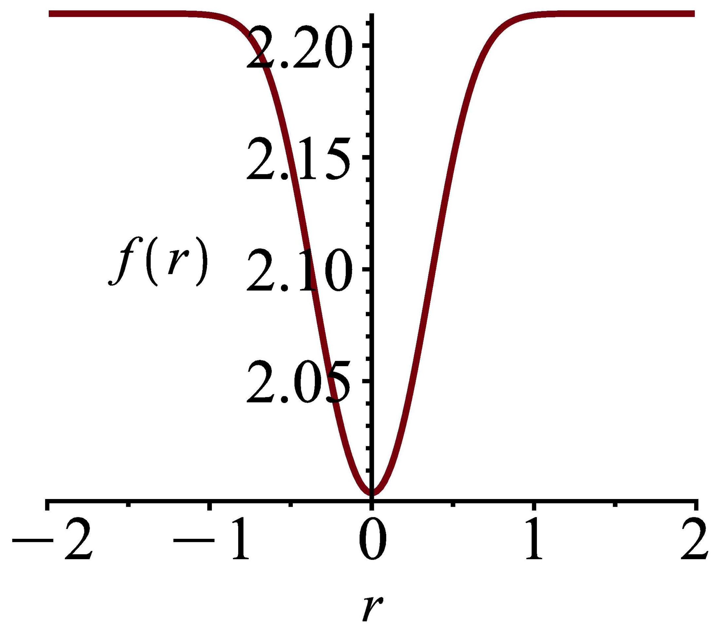
We solve this problem and we have:
where:
and:
and is the so-called Lambert function, which satisfies the equation . For :
We present a figure of this above solution in Figure 1.
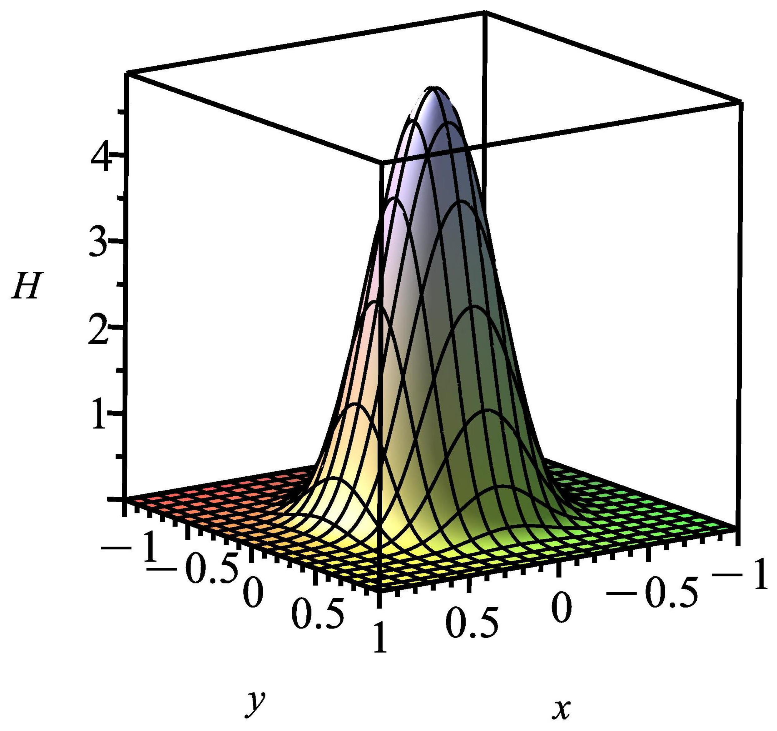
If we insert the found solution of the Cauchy problem into the ungauged and gauged Hamiltonian densities (58) and (60), correspondingly, then the ungauged Hamiltonian density is nonzero (Figure 2).
As we can see from the figures, both the found solution and the density of the ungauged Hamiltonian, corresponding to this, are localized. Thus, we can tell this solution is a soliton solution (or, at least, a soliton-like solution). For this solution, the gauged Hamiltonian density is zero (of course, the condition (61) and Bogomolny Equation (62) hold):
Thus, we can see here the degeneracy of the Hamiltonian (the problem of a degenerate Hamiltonian, in the case of theory of gravity, was investigated in [81]; in [82], the existence of an infinite number of Lagrangians for a given second-order ODE was proven). This corresponds to the fact that if we consider two versions of a field-theoretical Lagrangian, ungauged and gauged on total derivatives of any function of field variables, then the energy-momentum tensors corresponding to each of these Lagrangians will be different, ref. [83]. The term does not change the Euler–Lagrange equations, but has an impact on the energy of the ground state of the medium, ref. [84]. Such a term can appear only in crystals not possessing the inversion center, and this causes the spiral ordering of magnetic moments, ref. [84] (and the references [1,2,3,4] cited there; the numbers of these references are of the reference [84] ).
Hence, we mention the breaking of some symmetry: the Euler–Lagrange equations are the same for both Hamiltonians, gauged and ungauged; however, on the other hand, the density of the ungauged Hamiltonian is nonzero and the density of the gauged Hamiltonian is zero.
The effect of vanishing of energy-momentum tensor (when topological invariants occur in an action functional), was established in [57], for some two Yang-Mills family models (and for certain other field-theoretical models in refs. [85,86,87]). However, this had been done there for a version of BPS equations derived by using the method of classical completing action functional to square, so the forms of the invariants used there, had been special (in contrary to this paper, where we have used generalized forms of the invariants). The effect of degeneracy of hamiltonian for the restricted baby Skyrme model (and the exact localized solution for this), presented in this paper, had not been presented elsewhere (to our best knowledge).
6. Conclusions
The first conclusion concerns the possibility to solve the ordinary differential equations subjected to the strong necessary conditions. In the case of linear ODE, the new solution of the Cauchy problem associated with the Bogomolny equation for harmonic oscillator is given by (33) and (34). This solution depends not only on , but also on the mass m.
The Formulas (47) and (48) establish the Cauchy–Riemann system, which is a starting point for the theory of analytic functions. Because of the Riemann theorem, this may be a step to the investigations of conformal maps.
Moreover, as far as the Cauchy problems for the continuous Heisenberg model and for the restricted baby Skyrme model are concerned, after using strong necessary conditions and deriving the Bogomolny equation for this problem, one can formulate the Cauchy problem and solve it. One can also consider a possibility of an extension of the obtained solution by applying the so-called semi-strong necessary conditions concept (this concept was presented in [41]).
We have also obtained a localized solution of the Cauchy problem of Bogomolny equation for the restricted baby Skyrme model. An example of such a solution (soliton solution or, at least, a soliton-like solution) is given by (71). The density of the ungauged Hamiltonian for this solution is localized.
Moreover, we have also shown, in the example of the restricted baby Skyrme model, that in the case of Bogomolny equations, there exists some degeneracy of the Hamiltonian, i.e., the values of Hamiltonians, both ungauged and gauged ones, are different for the solution of the Cauchy problem for Bogomolny equations, and both of these Hamiltonians generate the same Euler–Lagrange equations.
One can say that some symmetry has been broken here: the Euler–Lagrange equations are the same for both Hamiltonians, gauged and ungauged; however, on the other hand, the density of the ungauged Hamiltonian is nonzero and the density of the gauged Hamiltonian is zero. It is worth mentioning here that, as was shown in [88], both Lagrangians (those gauged on the total derivative of a function of field variables and ungauged ones) lead to equivalent quantum field theories.
Funding
This research received no external funding.
Data Availability Statement
Data supporting results reported in this paper, can be found in appropriate sources mentioned in the section “References”.
Acknowledgments
The author thanks K. Sokalski for very fruitful comments and discussions. The author is also indebted to K. Pomorski for some very valuable remarks. The author is also grateful to Z. Lisowski (died in 2021) for very inspiring discussions. Parts of the computations were carried out using Maple Waterloo Software on the computer “mars” (grant nr MNiSW/IBM_BC_HS21/AP/057/2008) in ACK-CYFRONET AGH in Cracow, owing to a financial support provided by The Pedagogical University of Cracow within a research project (the leader of this project: K. Rajchel). This research was also supported partially by PL-Grid Infrastructure. Other parts of the computations were carried out using Maple Waterloo Software, owing to financial support from University Research Project number WPBU/2022/04/00319. This research was also carried out within the University Research Project number WPBU/2023/04/00009. The author thanks also the reviewers for their valuable remarks.
Conflicts of Interest
The author declares no conflict of interest.
References
- Adomian, G. Solving Frontiers Problems of Physics: The Decomposition Method; Springer Science+Business Media: Dordrecht, The Netherlands, 1994. [Google Scholar]
- Atmaja, A.N.; Ramadhan, H.S. Bogomol’nyi equations of classical solutions. Phys. Rev. 2014, D90, 105009. [Google Scholar] [CrossRef]
- Atmaja, A.N. A method for BPS equations of vortices. Phys. Lett. 2017, B768, 351. [Google Scholar] [CrossRef]
- Benci, V.; Fortunato, D. Variational Methods in Nonlinear Field Equations. Solitary Waves, Hylomorphic Solutions and Vortices; Springer International Publishing: Cham, Switzerland, 2014. [Google Scholar]
- Bluman, G.W.; Cheviakov, A.F.; Anco, S.C. Applications of Symmetry Methods to Partial Differential Equations; Springer Science+Business Media: Dordrecht, The Netherlands, 2010. [Google Scholar]
- Cieśliński, J. The Darboux-Bianchi-Bäcklund transformation and soliton surfaces. In Proceedings of the Nonlinearity & Geometry, Proceedings of First Non-Orthodox School; Cieśliński, J., Wójcik, D., Eds.; PWN: Warszawa, Poland, 1998; p. 81. [Google Scholar]
- Conte, R. Exact solutions of nonlinear partial differential equations by singularity analysis. In Lecture Notes in Physics, Proceedings of the Direct and Inverse Methods in Nonlinear Evolution Equations; Greco, A.M., Ed.; Springer: Berlin/Heidelberg, Germany, 2003; Volume 632, p. 1. [Google Scholar]
- Debnath, L. Nonlinear Partial Differential Equations for Scientists and Engineers; Springer Science+Business Media, Birkhäuser: Basel, Switzerland, 2012. [Google Scholar]
- Doliwa, A. Minimal surfaces, holomorphic curves and Toda systems. In Proceedings of the Nonlinearity & Geometry, Proceedings of First Non-Orthodox School; Cieśliński, J., Wójcik, D., Eds.; PWN: Warszawa, Poland, 1998; p. 227. [Google Scholar]
- Elzaki, T.M.; Biazar, J. Homotopy Perturbation Method and Elzaki Transform for Solving System of Nonlinear Partial Differential Equations. World Appl. Sci. J. 2013, 24, 944. [Google Scholar]
- Feng, Z.S. The first-integral method to study the Burgers–Korteweg–de Vries equation. J. Phys. A Math. Gen. 2002, 35, 343. [Google Scholar] [CrossRef]
- Fushchich, W.I.; Shtelen, W.M.; Serov, N. Symmetry Analysis and Exact Solutions of Equations of Nonlinear Mathematical Physics; Kluwer Academic Publishers: Dordrecht, The Netherlands, 1993. [Google Scholar]
- Gaeta, G. Nonlinear Symmetries and Nonlinear Equations; Springer Science+Business Media: Dordrecht, The Netherlands, 1994. [Google Scholar]
- Goldstein, P. Painleve test: Standard gun of integrability hunter. In Proceedings of the Nonlinearity & Geometry, Proceedings of First Non-Orthodox School; Cieśliński, J., Wójcik, D., Eds.; PWN: Warszawa, Poland, 1998; p. 207. [Google Scholar]
- Gu, C.; Hu, H.; Zhou, Z. Darboux Transformations in Integrable Systems. Theory and Their Applications to Geometry; Springer: Berlin/Heidelberg, Germany, 2005. [Google Scholar]
- Kudryashov, N.A. Analytic Theory of Nonlinear Differential Equations; Moscow-Izhevsk, Institute of Computer Studies: Izhevsk, Russia, 2004. (In Russian) [Google Scholar]
- Magri, F.; Falqui, G.; Pedroni, M. The method of Poisson pairs in the theory of nonlinear PDEs. In Lecture Notes in Physics, Proceedings of the Direct and Inverse Methods in Nonlinear Evolution Equations; Greco, A.M., Ed.; Springer: Berlin/Heidelberg, Germany, 2003; Volume 632, p. 85. [Google Scholar]
- Meleshko, S.V. Methods for Constructing Exact Solutions of Partial Differential Equations; Springer: Berlin/Heidelberg, Germany, 2005. [Google Scholar]
- Musette, M. Nonlinear superposition formulae of integrable partial differential equations by the singular manifold method. In Lecture Notes in Physics, Proceedings of the Direct and Inverse Methods in Nonlinear Evolution Equations; Greco, A.M., Ed.; Springer: Berlin/Heidelberg, Germany, 2003; Volume 632, p. 137. [Google Scholar]
- Krasil’shchik, I. Symmetries and recursion operators for soliton equations. In Proceedings of the Nonlinearity & Geometry, Proceedings of First Non-Orthodox School; Cieśliński, J., Wójcik, D., Eds.; PWN: Warszawa, Poland, 1998; p. 141. [Google Scholar]
- Nieszporski, M.; Sym, A. Weingarten congruences and non-auto-Backlund transformations for hyperbolic surfaces. In Proceedings of the Nonlinearity & Geometry, Proceedings of First Non-Orthodox School; Cieśliński, J., Wójcik, D., Eds.; PWN: Warszawa, Poland, 1998; p. 37. [Google Scholar]
- Olver, P.J. Applications of Lie Groups to Differential Equations; Springer: Berlin/Heidelberg, Germany, 1986. [Google Scholar]
- Polyanin, A.D.; Zaitsev, V.F. Handbook of Nonlinear Partial Differential Equations; CRC Press Taylor & Francis Group: Boca Raton, FL, USA, 2012. [Google Scholar]
- Rajchel, K.; Szczȩsny, J. New method to solve certain differential equations. Ann. Univ. Paedagog. Crac. Stud. Math. 2016, XV, 107. [Google Scholar] [CrossRef]
- Rubina, L.I.; Ul’yanov, O.N. On one approach to solving nonhomogeneous partial differential equations. Vestn. Udmurtsk. Univ. Mat. Mekh. Komp. Nauki 2017, 27, 355. [Google Scholar] [CrossRef]
- Satsuma, J. Hirota bilinear method for nonlinear partial differential equations. In Lecture Notes in Physics, Proceedings of the Direct and Inverse Methods in Nonlinear Evolution Equations; Greco, A.M., Ed.; Springer: Berlin/Heidelberg, Germany, 2003; Volume 632, p. 171. [Google Scholar]
- Stȩpień, T. Some decomposition method for analytic solving of certain nonlinear partial differential equations in physics with applications. J. Comp. Appl. Math. 2010, 233, 1607. [Google Scholar] [CrossRef]
- Stȩpień, T. Some Exact Soluions for ABC equations and Martínez Alonso Shabat Equations. J. Geom. Symm. Phys. 2023, 66, 47. [Google Scholar] [CrossRef]
- Vitanov, N.K.; Dimitrova, Z.I.; Vitanov, K.N. Modified method of simplest equation for obtaining exact analytical solutions of nonlinear partial differential equations: Further development of the methodology with applications. Appl. Math. Comp. 2015, 269, 363–378. [Google Scholar] [CrossRef]
- Wietecha, T.; Sokalski, K. Plus-minus algorithm—A method for derivation of the Bäcklund transformations. J. Symb. Comp. 2009, 44, 1511. [Google Scholar] [CrossRef]
- Winternitz, P. Lie groups, singularities and solutions of nonlinear partial differential equations. In Lecture Notes in Physics, Proceedings of the Direct and Inverse Methods in Nonlinear Evolution Equations; Greco, A.M., Ed.; Springer: Berlin/Heidelberg, Germany, 2003; Volume 632, p. 223. [Google Scholar]
- Zakharov, V.E.; Shabat, A.B. A scheme for integrating the nonlinear equations of mathematical physics by the method of the inverse scattering problem I. Funct. Anal. Appl. 1977, 11, 226. [Google Scholar]
- Zhang, Z.Y.; Zhong, J.; Dou, S.S.; Liu, J.; Peng, D.; Gao, T. First integral method and exact solutions to nonlinear partial differential equations arising in mathematical physics. Rom. Rep. Phys. 2013, 65, 1155. [Google Scholar]
- Fedorchuk, V.M.; Fedorchuk, V.I. Reduction of the (1+ 3)-Dimensional Inhomogeneous Monge–Ampère Equation to First-Order Partial Differential Equations. Ukr. Math. J. 2022, 74, 472. [Google Scholar] [CrossRef]
- Adam, C.; Santamaria, F. The first-order Euler-Lagrange equations and some of their uses. J. High Energ. Phys. 2016, 2016, 047. [Google Scholar] [CrossRef]
- Sokalski, K. Instantons in Anisotropic Ferromagnets. Acta Phys. Pol. 1979, A56, 571. [Google Scholar]
- Sokalski, K. Dynamical stability of instantons. Phys. Lett. 1981, A81, 102. [Google Scholar] [CrossRef]
- Sokalski, K. Instantons in Three-Dimensional Heisenberg Ferromagnets. Acta Phys. Pol. 1984, A65, 457. [Google Scholar]
- Jochym, P.T.; Sokalski, K. Variational approach to the Bogomolny separation. J. Phys. A Math. Gen. 1993, 26, 3837. [Google Scholar] [CrossRef]
- Sokalski, K.; Stȩpień, T.; Sokalska, D. The existence of Bogomolny decomposition by means of strong necessary conditions. J. Phys. 2002, A35, 6157. [Google Scholar] [CrossRef]
- Sokalski, K.; Wietecha, T.; Lisowski, Z. Variational Approach to the Bäcklund Transformations. Acta Phys. Pol. 2001, B32, 17. [Google Scholar]
- Sokalski, K.; Wietecha, T.; Lisowski, Z. A Concept of Strong Necsseary Conditions in Nonlinear Field Theory. Acta Phys. Pol. 2001, B32, 2771. [Google Scholar]
- Sokalski, K.; Wietecha, T.; Lisowski, Z. Unified Variational Approach to the Bäcklund Transformations and the Bogomolny Decomposition. Int. J. Theor. Phys. Group Theory Nonlinear Opt. NOVA 2002, 9, 331. [Google Scholar]
- Sokalski, K.; Wietecha, T.; Sokalska, D. Existence of dual equations by means of strong necessary conditions-Analysis of integrability of partial differential nonlinear equations. J. Nonlinear Math. Phys. 2005, 12, 31. [Google Scholar] [CrossRef]
- Stȩpień, T. Bogomolny Decomposition in the Context of the Concept of Strong Necessary Conditions. Ph.D. Dissertation, Jagiellonian University, Kraków, Poland, Marian Smoluchowski Institute of Physics, Department of Mathematics, Physics and Astronomy, Cracow, Poland, 2003. [Google Scholar]
- Stȩpień, T.; Sokalska, D.; Sokalski, K. The Bogomolny decomposition for systems of two generalized nonlinear partial differential equations of the second order. J. Nonlinear Math. Phys. 2009, 16, 25. [Google Scholar] [CrossRef]
- Stȩpień, T. On Bogomolny Decompositions for the Baby Skyrme Models. In Proceedings of the Geometric Methods in Physics, XXXI Workshop; Białowieża, Poland, 24–30 June 2012, Kielanowski, P., Ali, S.T., Odesskii, A., Odzijewicz, A., Schlichenmaier, M., Voronov, T., Eds.; Trends in Mathematics; Birkhäuser, Springer: Basel, Switzerland, 2013; pp. 229–237. [Google Scholar]
- Stȩpień, T. The Existence of Bogomolny Decompositions for Gauged O(3) Nonlinear “Sigma” Model and for Gauged Baby Skyrme Models. Acta Phys. Pol. B 2015, 46, 999. [Google Scholar] [CrossRef]
- Stȩpień, T. Bogomolny equation for the BPS Skyrme model from strong necessary conditions. J. Phys. A 2016, 49, 175202. [Google Scholar] [CrossRef]
- Stȩpień, T. Bogomolny equations in certain generalized baby BPS Skyrme models. J. Phys. A 2018, 51, 015208. [Google Scholar] [CrossRef]
- Stȩpień, T. Bogomolny equations for the BPS Skyrme models with impurity. J. High Energ. Phys. 2020, 2020, 140. [Google Scholar] [CrossRef]
- Stȩpień, T.; Pomorski, K. Bogomolny approach in description of superconducting structures. arXiv 2023, arXiv:2308.09172. [Google Scholar]
- Szafirski, B.; Institute of Mathematics, Jagiellonian University, Kraków, Poland. Personal Communication, 2001.
- Stȩpień, T. Strong necessary conditions and Cauchy problem. arXiv 2019, arXiv:1912.02609v2. [Google Scholar]
- Bogomolny, E.B. The stability of classical solutions. Sov. J. Nucl. Phys. 1976, 24, 449. [Google Scholar]
- Belavin, A.A.; Polyakov, A.M.; Schwartz, A.S.; Tyupkin, Y.S. Pseudoparticle solutions of the Yang-Mills equations. Phys. Lett. 1975, B59, 85. [Google Scholar] [CrossRef]
- Hosoya, A. On Vanishing of Energy-Momentum Tensor for a Class of Instanton-Like Solutions. Prog. Theor. Phys. 1978, 59, 1781. [Google Scholar] [CrossRef]
- Białynicki-Birula, I. On the stability of solitons. In Lecture Notes in Physics, Proceedings of the Nonlinear Problems in Theoretical Physcis, Jaca, Spain, June 1978; Rañada, A.F., Ed.; Birkhäuser, Springer: Basel, Switzerland, 1979; Volume 98, p. 15. [Google Scholar]
- Meissner, K.A. Classical Field Theory; PWN: Warszawa, Poland, 2013. (In Polish) [Google Scholar]
- Belavin, A.A.; Polyakov, A.M. Metastable states of two dimensional isotropic ferromagnets. JETP Lett. 1975, 22, 245. [Google Scholar]
- Balakrishnan, R.; Bishop, A.R.; Dandoloff, R. Geometric phase in the classical continuous antiferromagnetic Heisenberg spin chain. Phys. Rev. Lett. 1990, 64, 2107. [Google Scholar] [CrossRef]
- Balakrishnan, R.; Dandoloff, R.; Saxena, A. Exact hopfion vortices in a 3D Heisenberg ferromagnet. Phys. Lett. A 2023, 480, 128975. [Google Scholar] [CrossRef]
- Felsager, B. Geometry, Particles and Fields; Springer Science+Business Media: New York, NY, USA, 1998. [Google Scholar]
- Morandi, G. The Role of Topology in Classical and Quantum Physics; Lecture Notes in Physics; Springer: Berlin/Heidelberg, Germany, 1992. [Google Scholar]
- Arodź, H.; Hadasz, L. Lectures on Classical and Quantum Theory of Fields; Springer: Berlin/Heidelberg, Germany, 2017. [Google Scholar]
- Bogoliubov, N.N.; Shirkov, D.V. Introduction to the Theory of Quantized Fields. In Nikolai Nikolaevich Bogoliubov. Collection of Scientific Works; Sukhanov, A.D., Ed.; Nauka: Moscow, Russia, 2008; Volume 10. (In Russian) [Google Scholar]
- Landau, L.D.; Lifshitz, E.M. Mechanics; PWN: Warszawa, Poland, 2012. (In Polish) [Google Scholar]
- Gignoux, C.; Silvestre-Brac, B. Solved Problems in Lagrangian and Hamiltonian Mechanics; Springer Science+Business Media B.V.: Berlin/Heidelberg, Germany, 2009. [Google Scholar]
- Knudsen, J.M.; Hjorth, P.G. Elements of Newtonian Mechanics. Including Nonlinear Dynamics; Springer: Berlin/Heidelberg, Germany, 2000. [Google Scholar]
- Cieśliński, J.L. On the exact discretization of the classical harmonic oscillator equation. J. Diff. Equ. Appl. 2013, 17, 1673. [Google Scholar] [CrossRef]
- Saxena, A.; Kevrekidis, P.; Cuevas-Maraver, J. Nonlinearity and Topology. In Emerging Frontiers in Nonlinear Science; Kevrekidis, P., Cuevas-Maraver, J., Saxena, A., Luo, A.C.J., Eds.; Nonlinear Systems and Complexity Series; Springer Nature Switzerland AG: Cham, Switzerland, 2020; Chapter 2, Volume 32, pp. 25–53. [Google Scholar]
- Skyrme, T.H.R. A non-linear field theory. Proc. R. Soc. Lond. 1961, A260, 127–138. [Google Scholar]
- Skyrme, T.H.R. A unified field theory of mesons and baryons. Nucl. Phys. 1962, 31, 556. [Google Scholar] [CrossRef]
- Makhankov, V.G.; Rybakov, Y.P.; Sanyuk, V.I. The Skyrme Model: Fundamentals, Methods, Applications; Springer: Berlin/Heidelberg, Germany, 1993. [Google Scholar]
- Sondhi, S.L.; Karlhede, A.; Kivelson, S.A.; Rezayi, E.H. Skyrmions and the crossover from the integer to fractional quantum Hall effect at small Zeeman energies. Phys. Rev. B 1993, 47, 16419. [Google Scholar] [CrossRef]
- Schwindt, O.; Weidig, T. Towards a phase diagram of the 2D Skyrme model. Europhys. Lett. 2001, 55, 633. [Google Scholar] [CrossRef]
- Weidig, T. The baby Skyrme models and their multi-skyrmions. Nonlinearity 1999, 12, 1489. [Google Scholar] [CrossRef]
- Hu, H.; Hu, K. Existence of Solutions for a Baby-Skyrme Model. J. Appl. Math. 2014, 2014, 1. [Google Scholar] [CrossRef]
- Adam, C.; Romańczukiewicz, T.; Sanchez-Guillen, J.; Wereszczyński, A. Investigation of restricted baby Skyrme models. Phys. Rev. 2010, D81, 085007. [Google Scholar] [CrossRef]
- Speight, J.M. Compactons and semi-compactons in the extreme baby Skyrme model. J. Phys. A 2010, 43, 405201. [Google Scholar] [CrossRef]
- Sanyal, A.K. Degenerate Hamiltonian operator in higher-order canonical gravity—The problem and a remedy. Ann. Phys. 2019, 411, 167971. [Google Scholar] [CrossRef]
- Del Castillo, G.F.T.; Mirón, C.A.; Rojas, R.I.B. Variational symmetries of Lagrangians. Riv. Mexic. Fis. E 2013, 59, 140. [Google Scholar]
- Arodź, H. Lectures on Field Theory. Delivered at Institute of Physics, Jagiellonian University 1997/1998. Unpublished.
- Kiselev, V.V.; Batalov, S.V. Nonlinear interference of solitons and waves in the magnetic domain structure. Theor. Math. Phys. 2023, 214, 369. [Google Scholar] [CrossRef]
- Dimopoulos, S.; Eguchi, T. Virial theorems on instantons. Phys. Lett. 1977, 66B, 480. [Google Scholar] [CrossRef]
- De Vega, H.J.; Schaposnik, F.A. Classical vortex solution of the Abelian Higgs model. Phys. Rev. D 1976, 14, 1100. [Google Scholar] [CrossRef]
- Belavin, A.A.; Burlankov, D.E. The renormalisable theory of gravitation and the einstein equations. Phys. Lett. 1976, 58A, 7. [Google Scholar] [CrossRef]
- Faddeev, L.D.; Jackiw, R. Hamiltonian reduction of unconstrained and constrained systems. Phys. Rev. Lett. 1988, 60, 1692. [Google Scholar] [CrossRef]
Figure 1.
Figure of solution (71).
Figure 1.
Figure of solution (71).

Figure 2.
The figure of the ungauged Hamiltonian density for solution (71).
Figure 2.
The figure of the ungauged Hamiltonian density for solution (71).

Disclaimer/Publisher’s Note: The statements, opinions and data contained in all publications are solely those of the individual author(s) and contributor(s) and not of MDPI and/or the editor(s). MDPI and/or the editor(s) disclaim responsibility for any injury to people or property resulting from any ideas, methods, instructions or products referred to in the content. |
© 2023 by the author. Licensee MDPI, Basel, Switzerland. This article is an open access article distributed under the terms and conditions of the Creative Commons Attribution (CC BY) license (https://creativecommons.org/licenses/by/4.0/).
Share and Cite
MDPI and ACS Style
Stȩpień, Ł.T. Strong Necessary Conditions and the Cauchy Problem. Symmetry 2023, 15, 1622. https://doi.org/10.3390/sym15091622
AMA Style
Stȩpień ŁT. Strong Necessary Conditions and the Cauchy Problem. Symmetry. 2023; 15(9):1622. https://doi.org/10.3390/sym15091622
Chicago/Turabian StyleStȩpień, Łukasz T. 2023. "Strong Necessary Conditions and the Cauchy Problem" Symmetry 15, no. 9: 1622. https://doi.org/10.3390/sym15091622
Note that from the first issue of 2016, this journal uses article numbers instead of page numbers. See further details here.