Recent Developments in Iterative Algorithms for Digital Metrics

Abstract

This paper aims to provide a comprehensive analysis of the advancements made in understanding Iterative Fixed-Point Schemes, which builds upon the concept of digital contraction mappings. Additionally, we introduce the notion of an Iterative Fixed-Point Schemes in digital metric spaces. In this study, we extend the idea of Iteration process Mann, Ishikawa, Agarwal, and Thakur based on the ϝ-Stable Iterative Scheme in digital metric space. We also design some fractal images, which frame the compression of Fixed-Point Iterative Schemes and contractive mappings. Furthermore, we present a concrete example that exemplifies the motivation behind our investigations. Moreover, we provide an application of the proposed Fractal image and Sierpinski triangle that compress the works by storing images as a collection of digital contractions, which addresses the issue of storing images with less storage memory in this paper.

1. Introduction and Preliminaries

In recent years, Rosenfeld [1] introduced the concept of the digital image, laying the foundation for Boxer’s [2] development of the topological notion of digital representation. Subsequently, Ege and Karaca [3,4,5,6] defined a digital metric space, offering a unified approach that has shed new light on the Banach contraction principle. This framework is particularly useful for measuring distances and similarities between points or patterns within a digital image. As a result, in this research, iterative schemes are employed to reduce data size or the dimension of picture files in digital contraction mappings and its applications. These schemes efficiently compress an image by iteratively refining approximations until a close match to the original image is achieved.

Now, we review some fundamental aspects of digital images, digital metric space, and ϝ-stable iterative scheme for the main continuation of our theoretical and geometrically analysis.

Definition 1

([6]). Let r, n be positive integers with $1\le r\le n$ in such a way that

$$\zeta =({\zeta }_1,{\zeta }_2,\dots ,{\zeta }_n),\kappa =({\chi }_1,{\chi }_2,\dots ,{\chi }_n)\in {\mathbb{Z}}^n.$$

where ζ and κ are ${\varrho }_r$-adjacent, if there is r indices τ such that $|{\zeta }_{\tau }-{\chi }_{\tau }|=1$ and for every other indices l such that

$$|{\zeta }_{\tau }-{\chi }_{\tau }|\ne 1,{\zeta }_l={\chi }_l.$$

There are some facts can be derived from Definition 1:

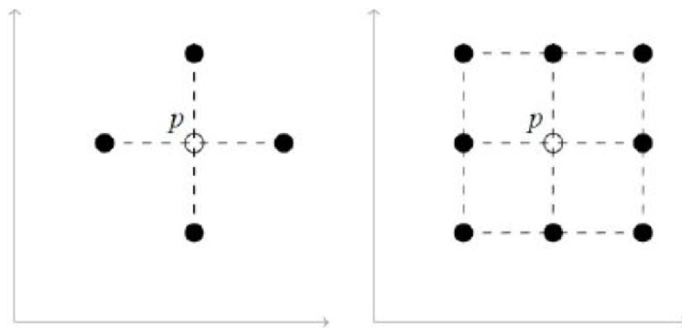
• Two points $\zeta$ and $\chi$ in Z are 2-adjacent, if $|\zeta -\chi |=1$ (see Figure 1).
  

  Figure 1. 2-adjacent.
• Two points $\zeta$ and $\chi$ in $Z^2$ are 8-adjacent, if they are distinct and differ by at most 1 in each coordinate.
• Two points $\zeta$ and $\chi$ in $Z^2$ are 4-adjacent, if they are 8-adjacent and differ in exactly one coordinate (see Figure 2).
  

  Figure 2. 4-adjacent and 8-adjacent.
• Two points $\zeta$ and $\chi$ in $Z^3$ are 26-adjacent, if they are distinct and differ by at most 1 in each coordinate.
• Two points $\zeta$ and $\chi$ in $Z^3$ are 18-adjacent, if they are 26-adjacent and differ at most two coordinates.
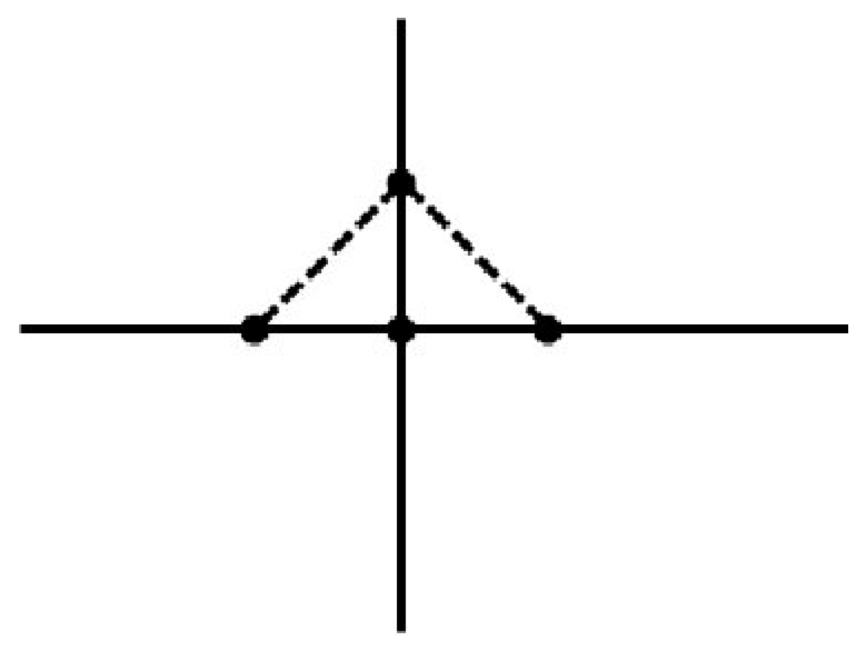
• Two points $\zeta$ and $\chi$ in $Z^3$ are 6-adjacent, if they are 18-adjacent and differ in exactly one coordinate (see Figure 3).
  

  Figure 3. 6-adjacent, 18-adjacent, and 26-adjacent.

Definition 2

([6]). Digital image is a graph $(D,\varrho )$, where ϱ is an adjacency relation, and D is a finite subset of Zⁿ for some positive integer n.

Definition 3

([6]). A ϱ-neighbor of $\zeta \in Z^n$ is a point of $Z^n$ that is ϱ-adjacent to ζ, where $\varrho \in \{2,4,6,8,18,26\}$ and $n\in \{1,2,3\}$.

Definition 4

([6]). The set $N_{\varrho }\left(\zeta \right)=\{\chi$|χ is ϱ-neighbor of ζ} is called the ϱ-neighborhood of ζ.

Definition 5

([6]). A digital interval is defined by ${[i,j]}_Z=\{\kappa \in Z$|$i\le \kappa \le j\}$, where $i,j\in Z$ and $i<j$.

A digital image $D\subset Z^n$ is $\varrho$–connected [6] if and only if for every pair of different points $𝚤,j\in D$, there is a set $\{{𝚤}_0,{𝚤}_1,\dots ,{𝚤}_r\}$ of points of a digital image X such that $𝚤={𝚤}_0$, $j={𝚤}_r$ and ${𝚤}_i$ and ${𝚤}_{i+1}$ are $\varrho$-neighbors where $i=0,1,\dots ,r-1$.

Definition 6

([7]). Let $(D,{\varrho }_0)\subset Z^{p_0}$, and $(M,{\varrho }_1)\subset Z^{p_1}$ be digital images and $\mu :D\to M$ be a function’

• If for every ${\varrho }_0$-connected of $X\subset D$, $\mu \left(X\right)$ is a ${\varrho }_1$-connected of $M\subset D$, then μ is said to be $({\varrho }_0,{\varrho }_1)$-continuous [8].
• μ is $({\varrho }_0,{\varrho }_1)$-continuous [8] if and only if for every ${\varrho }_0$-adjacent points $\{{𝚤}_0,{𝚤}_1\}$ of D, either $\mu \left({𝚤}_0\right)=\mu \left({𝚤}_1\right)$ or $\mu \left({𝚤}_0\right)$ and $\mu \left({𝚤}_1\right)$ are ${\varrho }_1$-adjacent in M.
• If μ is $({\varrho }_0,{\varrho }_1)$-continuous, bijective, and ${\mu }^{-1}$ is $({\varrho }_1,{\varrho }_0)$-continuous, then μ is called $({\varrho }_0,{\varrho }_1)$-isomorphism [2], that is $D{\cong }_{({\varrho }_0,{\varrho }_1)}M$.

Definition 7

([7]). Let $D\subset Z^n$, g be the Euclidean metric on $Z^n$. Suppose metric space $(D,g)$ and $(D,\varrho )$ is a digital image with ϱ-adjaceny, then $(D,g,\varrho )$ is called a digital metric space.

Definition 8

([6]). A sequence $\left\{{𝚤}_p\right\}$ in digital metric space $(D,g,\varrho )$ converges to $q\in D,$ if for all $ϵ>0$, there exists $\eta \in N$ such that for all $p>\eta$, then

$$g({𝚤}_p,q)<ϵ.$$

Definition 9

([6]). Let $(D,g,\varrho )$ be a digital metric space and $\mu :(D,g,\varrho )\to (D,g,\varrho )$ be a self digital mapping. If there is $L\in (0,1)$ such that for all $𝚤,j\in D$,

$$g\left(\mu \right(𝚤),\mu (j\left)\right)\le Lg(𝚤,j),$$

then μ is called a digital contraction map.

Proposition 1

([6]). Every digital contraction map is digitally continuous.

Theorem 1

([9]). Digital metric space $(D,g,\varrho )$ is a complete metric space.

Hicks and Harder [10] presented a stability result for iterative processes in a complete metric space, which can be restated as follows:

Definition 10

([10]). Let $(D,g)$ be a complete metric space, $\mathsf{𝟊}:D\to D$ be a self mapping, and ${𝚤}_{n+1}=f(\mathsf{𝟊},{𝚤}_n)$ be a iterative procedure. Suppose that $Fix\left(\mathsf{𝟊}\right)\ne \varphi$, the set of fixed point, and sequence ${𝚤}_n$ converges to $l\in Fix\left(\mathsf{𝟊}\right)$.

Let a sequence $\left\{j_n\right\}\subset D$ and ${ϵ}_n=g(j_{n+1},f(\mathsf{𝟊},j_n))$. If ${lim}_{n\to \infty }{ϵ}_n=0$ such that ${lim}_{n\to \infty }{j}_n=l$, then ${𝚤}_{n+1}=f(\mathsf{𝟊},{𝚤}_n)$ is said to be $\mathsf{𝟊}$-stable. See more details in [10,11].

Osilike and Udomene [12] designed the following contractive condition, that is, for each $𝚤,j\in D$ there is constants $\eta \in [0,1)$ and $\widehat{L}\ge 0$ such that

$$g(\mathsf{𝟊}𝚤,\mathsf{𝟊}j)\le \widehat{L}\left(g(𝚤,\mathsf{𝟊}𝚤)\right)+\eta g(𝚤,j).$$

(1)

After, Osilike [12] established various stability results that generalize and extend many of the findings of Rhoades [11].

If $\widehat{L}=2\xi$ and $\eta =\xi ,$ where $\xi =max\{\eta ,\frac{\mu }{1-\mu },\frac{\nu }{1-\nu }\}$ and $0\le \xi <1$ then the contractive condition (1) restated to the Zamfirscu [13] contraction condition, that is,

$$g(\mathsf{𝟊}𝚤,\mathsf{𝟊}j)\le \xi g(𝚤,j)+2\xi \left(g\right(𝚤,\mathsf{𝟊}𝚤\left)\right).$$

(2)

Furthermore, if $\widehat{L}=0$ then (1) yield as

$$g(\mathsf{𝟊}𝚤,\mathsf{𝟊}j)\le \eta g(𝚤,j).$$

(3)

Berinde [14,15,16,17] established several generalizations of Banach’s fixed point theorem. In one of the results of Berinde [17], designed that ideas in the following frame of extension, that is, for each $𝚤,j\in D$, there exist $\eta \in [0,1)$ and $\widehat{L}\ge 0$ such that

$$g(\mathsf{𝟊}𝚤,\mathsf{𝟊}j)\le \widehat{L}\left(\alpha (𝚤,\mathsf{𝟊}𝚤)\right)+\eta A(𝚤,j).$$

(4)

where

$$A(𝚤,j)=max\{g(𝚤,j),g(𝚤,\mathsf{𝟊}𝚤),g(j,\mathsf{𝟊}j),\frac{1}{2}[g(𝚤,\mathsf{𝟊}j)+g(j,\mathsf{𝟊}𝚤)]\}$$

and

$$\alpha (𝚤,j)=min\left\{g\right(𝚤,\mathsf{𝟊}𝚤),g(j,\mathsf{𝟊}j),g(𝚤,\mathsf{𝟊}j),g(j,\mathsf{𝟊}𝚤\left)\right\}.$$

Pradip Debnath [18] introduced the following generalized Boyd–Wong-type contractive conditions and proved fixed-figure theorems in metric spaces. Suppose $\alpha :D\to D$ and upper semi-continuous functions $\Xi :[0,\infty )\to [0,\infty )$ with $0\le \Xi \left(s\right)<s$ for $s>0$ such that $\Xi \left(0\right)=0$. If there is ${\beta }_0\in D$ such that

$$\chi (\alpha \beta ,\beta )>0\Rightarrow \chi (\alpha \beta ,\beta )\le \Xi \left(\chi (\beta ,{\beta }_0)\right)$$

(5)

for all $\beta \in D$, then $\alpha$ is called a Boyd and Wong type ${\beta }_0$-contraction.

Amid the years, which have been failed since this hypothsis, a number of iteration techniques have been established to approximate non-expasive mappings. Mann’s iteration system [19] has been substantially used to approximate fixed point of non-expasive mappings. In this fashion of iterative system, the sequence $\left\{{𝚤}_n\right\}$ is procreated from an arbitrary point ${𝚤}_0\in D$; by the technique as follow:

$${𝚤}_{n+1}=(1-{\eta }_n){𝚤}_n+{\eta }_n\mathsf{𝟊}{𝚤}_n,{\eta }_n\in [0,1],$$

(6)

where $n=0,1,2,\dots ,\infty$.

Later on, Ishikawa [20] investigated the new iterative system which has been broadly used to approximate fixed point of non-expasive mappings. In this regard of iterative system the sequence $\left\{{𝚤}_n\right\}$ is given iteratively from ${𝚤}_0\in D$ by

$$\begin{array}{cc}\hfill {𝚤}_{n+1}& =(1-{\eta }_n){𝚤}_n+{\eta }_n\mathsf{𝟊}{j}_n;\hfill \\ \hfill j_n& =(1-{\mu }_n){𝚤}_n+{\mu }_n\mathsf{𝟊}{𝚤}_n,\hfill \end{array}$$

(7)

where ${\eta }_n,{\mu }_n\in [0,1]$ and n = 0,1, 2, ….

Hereafter, Agrawal et al. [21] provided the iteration system and they declared that the process of converges rate of analysis same as that of the Picard iterative system and faster than the Mann iterative system for contractions, where the sequence $\left\{{𝚤}_n\right\}$ is generated by

$$\begin{array}{cc}\hfill {𝚤}_{n+1}& =(1-{\eta }_n)\mathsf{𝟊}{𝚤}_n+{\eta }_n\mathsf{𝟊}{j}_n;\hfill \\ \hfill j_n& =(1-{\mu }_n){𝚤}_n+{\mu }_n\mathsf{𝟊}{𝚤}_n,\hfill \end{array}$$

(8)

where ${\eta }_n$, ${\mu }_n\in [0,1]$ for all $n\ge 0$ values.

B. S. Thakur et al. [22] introduce a new iteration process to approximate fixed point of nonexpasive mappings, where for any fixed value ${𝚤}_0\in D$ and the sequence $\left\{{𝚤}_n\right\}$ is construct by

$$\begin{array}{cc}\hfill {𝚤}_{n+1}& =(1-{\eta }_n)\mathsf{𝟊}{\zeta }_n+{\eta }_n\mathsf{𝟊}{j}_n;\hfill \\ \hfill j_n& =(1-{\mu }_n){\zeta }_n+{\mu }_n\mathsf{𝟊}{\zeta }_n;\hfill \\ \hfill {\zeta }_n& =(1-{\nu }_n){𝚤}_n+{\nu }_n\mathsf{𝟊}{𝚤}_n,\hfill \end{array}$$

(9)

for all $n\ge 0$, where ${\eta }_n$, ${\mu }_n$, and ${\nu }_n$ are in $[0,1]$.

Lemma 1

([14]). Let $\left\{{\epsilon }_n\right\}$ where $n=0,1,2,\dots ,\infty$ such that ${lim}_{n⟶\infty }{\nu }_n=0$ and $0\le \xi <1$, then for any sequence of positive numbers $\left\{b_n\right\}$ where n $=0,1,2$, …, satisfying

$$b_{n+1}\le \xi \left(b_n\right)+{\epsilon }_n,\forall n=0,1,2,\dots$$

(10)

then we have ${lim}_{n\to \infty }{b}_n=0$.

Definition 11.

Let $(D,\tilde{\mu },\varrho )$ be a digital metric space and $♢:D\times [0,1]\to D$ be a mapping such that $♢(l,\eta +\mu )=♢(l,\eta )+♢(l,\mu )$ and $♢(l,1)=l$. We say that a digital metric space have linear digital structure if for all $l,m,h,t\in D$ and $\eta ,\mu \in [0,1],$ if it satisfies,

$$\tilde{\mu }(♢(l,\eta )+♢(m,\mu ),♢(h,\eta )+♢(t,\mu ))\le \eta \tilde{\mu }(l,h)+\mu \tilde{\mu }(m,t).$$

(11)

Definition 12

([23]). Let $(D,\tilde{\mu },\varrho )$ be a digital metric space and ϝ a self-map of D. Let ${𝚤}_{n+1}$ be a iteration procedure defined as

$${𝚤}_{n+1}=f_{\mathsf{𝟊},{\alpha }_n}\left({𝚤}_n\right)$$

(12)

where ${\alpha }_n\in [0,1]$ and f is a function involving the digital structure. Suppose that $Fix\left(\mathsf{𝟊}\right)$, the fixed point set of ϝ, is nonempty and that ${𝚤}_n$ converges to a point $l\in Fix\left(\mathsf{𝟊}\right)$. Let $\left\{j_n\right\}\subset D$ and define ${ϵ}_n=\tilde{\mu }(j_{n+1},f_{\mathsf{𝟊},{\alpha }_n}\left(j_n\right))$. If ${lim}_{n\to \infty }{ϵ}_n=0$ implies that ${lim}_{n\to \infty }{j}_n=l$, then the iteration procedure ${𝚤}_{n+1}=f_{\mathsf{𝟊},{\alpha }_n}\left({𝚤}_n\right)$ is said to be ϝ-stable.

Motivated by the work of Berinde [17], we will use the following contractive condition: For a mapping $\mathsf{𝟊}:D⟶D$, there exists $\eta \in [0,1)$ and $L\ge 0$ such that for all $𝚤,j\in D$

$$\tilde{\mu }(\mathsf{𝟊}𝚤,\mathsf{𝟊}j)\le \eta \tilde{\mu }(𝚤,j)+L\left(m(𝚤,j)\right)$$

(13)

where,

$$\begin{array}{cc}\hfill m(𝚤,j)=& min\{\tilde{\mu }(𝚤,\mathsf{𝟊}𝚤),\tilde{\mu }(j,\mathsf{𝟊}j),\tilde{\mu }(𝚤,\mathsf{𝟊}j),\tilde{\mu }(j,\mathsf{𝟊}𝚤),\hfill \\ \hfill & \frac{1}{2}[\tilde{\mu }(𝚤,\mathsf{𝟊}j)+\tilde{\mu }(j,\mathsf{𝟊}𝚤)],\frac{1}{2}[\tilde{\mu }(𝚤,\mathsf{𝟊}𝚤)+\tilde{\mu }(j,\mathsf{𝟊}j)]\}.\hfill \end{array}$$

(14)

The contractive condition (13) is more general than the contractive conditions (1), (3), (2) and (4).

In this study, inspired by the concept of Mann, Ishikawa, Agarwal, and Thakur iterative procedure in the class of Banch spaces, we develop a new iterative procedure and design $\mathsf{𝟊}$-stability in the context of digital metric space. We also develop several fractal images to illustrate the compression of Fixed-Point Iterative Schemes and contractive mappings. Additionally, we present a specific example to demonstrate the motivation behind our investigations. Furthermore, we provide an application of the proposed Fractal image and Sierpinski triangle, which compress works by storing images as a collection of digital contractions, addressing the issue of storing images with less storage memory.

2. Main Results

First, in order to give our new extended iterative procedure in the class of digital metric space:

• Extended Mann (6) iteration process:

  $${𝚤}_{n+1}=♢({𝚤}_n,(1-{\eta }_n))+♢(\mathsf{𝟊}\left({𝚤}_n\right),{\eta }_n),{\eta }_n\in [0,1].$$

  (15)
• Extended Ishikawa (7) iteration process:

  $$\begin{array}{cc}\hfill {𝚤}_{n+1}& =♢({𝚤}_n,(1-{\eta }_n))+♢(\mathsf{𝟊}\left(j_n\right),{\eta }_n),{\eta }_n\in [0,1],\hfill \\ \hfill j_n& =♢({𝚤}_n,(1-{\mu }_n))+♢(\mathsf{𝟊}\left({𝚤}_n\right),{\mu }_n),{\mu }_n\in [0,1].\hfill \end{array}$$

  (16)
• Extended Agarwal (8) iteration process:

  $$\begin{array}{cc}\hfill {𝚤}_{n+1}& =♢(\mathsf{𝟊}{𝚤}_n,(1-{\eta }_n))+♢(\mathsf{𝟊}\left(j_n\right),{\eta }_n),{\eta }_n\in [0,1],\hfill \\ \hfill j_n& =♢({𝚤}_n,(1-{\mu }_n))+♢(\mathsf{𝟊}\left({𝚤}_n\right),{\mu }_n),{\mu }_n\in [0,1].\hfill \end{array}$$

  (17)
• Extended Thakur (9) iteration process:

  $$\begin{array}{cc}\hfill {𝚤}_{n+1}& =♢(\mathsf{𝟊}{z}_n,(1-{\eta }_n))+♢(\mathsf{𝟊}\left(j_n\right),{\eta }_n),{\eta }_n\in [0,1],\hfill \\ \hfill j_n& =♢(z_n,(1-{\mu }_n))+♢(\mathsf{𝟊}\left(z_n\right),{\mu }_n),{\mu }_n\in [0,1].\hfill \\ \hfill {\zeta }_n& =♢({𝚤}_n,(1-{\nu }_n))+♢(\mathsf{𝟊}\left({𝚤}_n\right),{\nu }_n),{\nu }_n\in [0,1].\hfill \end{array}$$

  (18)

Theorem 2.

Let $(D,\tilde{\mu },\varrho )$ be a digital metric space with linear digital structure ♢ and $\mathsf{𝟊}:D⟶D$ be a mapping that satisfies contractive condition (13). Suppose that ϝ has a fixed point l. For arbitrary setting ${𝚤}_0\in D$, let the sequence ${\left\{{𝚤}_n\right\}}_{n=0}^{\infty }$ is generated by the extended Mann iterative procedure (15), where ${\eta }_n\in [0,1]$ such that $0<\eta \le {\eta }_n$. Then, the extended Mann iteration is ϝ-stable.

Proof. 

Let $\left\{{𝚤}_n\right\}$ be the sequence in $\mathcal{D}$, where $n=0,1,2,\dots$ and define ${\epsilon }_n=\tilde{\mu }({𝚤}_{n+1},♢({𝚤}_n,(1-{\eta }_n))+♢(\mathsf{𝟊}\left({𝚤}_n\right),{\eta }_n))$. Suppose that ${lim}_{n\to \infty }{\epsilon }_n=0$. Then, we establish that ${lim}_{n\to \infty }{𝚤}_n=l$. By using condition (13). Thus, we have

$$\begin{array}{cc}\hfill \tilde{\mu }({𝚤}_{n+1},l)& \le \tilde{\mu }({𝚤}_{n+1},♢({𝚤}_n,(1-{\eta }_n))+♢(\mathsf{𝟊}\left({𝚤}_n\right),{\eta }_n))\hfill \\ \hfill & +\tilde{\mu }(♢({𝚤}_n,(1-{\eta }_n))+♢(\mathsf{𝟊}\left({𝚤}_n\right),{\eta }_n),l)\hfill \\ \hfill & =\tilde{\mu }(♢({𝚤}_n,(1-{\eta }_n))+♢(\mathsf{𝟊}\left({𝚤}_n\right),{\eta }_n),l)+{\epsilon }_n\hfill \\ \hfill & =\tilde{\mu }(♢({𝚤}_n,(1-{\eta }_n))+♢(\mathsf{𝟊}\left({𝚤}_n\right),{\eta }_n),♢(l,1))+{\epsilon }_n\hfill \\ \hfill & =\tilde{\mu }(♢({𝚤}_n,(1-{\eta }_n))+♢(\mathsf{𝟊}\left({𝚤}_n\right),{\eta }_n),♢(l,(1-{\eta }_n)+{\eta }_n)+{\epsilon }_n\hfill \\ \hfill & =\tilde{\mu }(♢({𝚤}_n,(1-{\eta }_n))+♢(\mathsf{𝟊}\left({𝚤}_n\right),{\eta }_n),♢(l,(1-{\eta }_n))+♢(l,{\eta }_n)+{\epsilon }_n\hfill \\ \hfill & \le (1-{\eta }_n)\tilde{\mu }({𝚤}_n,l)+{\eta }_n\tilde{\mu }(\mathsf{𝟊}\left({𝚤}_n\right),l)+{\epsilon }_n\hfill \\ \hfill & =(1-{\eta }_n)\tilde{\mu }({𝚤}_n,l)+{\eta }_n\tilde{\mu }(\mathsf{𝟊}\left({𝚤}_n\right),\mathsf{𝟊}\left(l\right))+{\epsilon }_n.\hfill \end{array}$$

Using (13), we have

$$\tilde{\mu }({𝚤}_{n+1},l)\le (1-{\eta }_n)\tilde{\mu }({𝚤}_n,l)+{\eta }_n[\xi \tilde{\mu }({𝚤}_n,l)+\mu m({𝚤}_n,l)]+{\epsilon }_n$$

Now, $m({𝚤}_n,l)=0$, and using (14), so

$$\begin{array}{cc}\hfill \tilde{\mu }({𝚤}_{n+1},l)& \le (1-{\eta }_n)\tilde{\mu }({𝚤}_n,l)+{\eta }_n\left(\xi \tilde{\mu }({𝚤}_n,l)\right)+{\epsilon }_n\hfill \\ \hfill & =[(1-{\eta }_n)+{\eta }_n\xi ]\tilde{\mu }({𝚤}_n,l)+{\epsilon }_n\hfill \\ \hfill & =[1-(1-\xi ){\eta }_n]\tilde{\mu }({𝚤}_n,l)+{\epsilon }_n.\hfill \end{array}$$

Therefore, we have

$$\tilde{\mu }({𝚤}_{n+1},l)\le [1-(1-\xi )\eta ]\tilde{\mu }({𝚤}_n,l)+{\epsilon }_n.$$

(19)

Therefore, since $0\le 1-(1-\xi )\eta <1$, applying Lemma 1 in (19), which yields ${lim}_{n⟶\infty }\tilde{\mu }({𝚤}_n,l)=0$, that is, ${lim}_{n⟶\infty }{𝚤}_n=l$. Conversely, ${lim}_{n⟶\infty }{𝚤}_n=l$. Then, we have to prove that ${lim}_{n⟶\infty }{\epsilon }_n=0$. Next,

$$\begin{array}{cc}\hfill {\epsilon }_n& =\tilde{\mu }({𝚤}_{n+1},♢({𝚤}_n,(1-{\eta }_n))+♢(\mathsf{𝟊}\left({𝚤}_n\right),{\eta }_n))\hfill \\ \hfill & \le \tilde{\mu }({𝚤}_{n+1},l)+\tilde{\mu }(l,♢({𝚤}_n,(1-{\eta }_n))+♢(\mathsf{𝟊}\left({𝚤}_n\right),{\eta }_n))\hfill \\ \hfill & =\tilde{\mu }({𝚤}_{n+1},l)+\tilde{\mu }(♢(l,1),♢({𝚤}_n,(1-{\eta }_n))+♢(\mathsf{𝟊}\left({𝚤}_n\right),{\eta }_n))\hfill \\ \hfill & \le \tilde{\mu }({𝚤}_{n+1},l)+\tilde{\mu }(♢(l,(1-{\eta }_n)+{\eta }_n),♢({𝚤}_n,(1-{\eta }_n))+♢(\mathsf{𝟊}\left({𝚤}_n\right),{\eta }_n))\hfill \\ \hfill & =\tilde{\mu }({𝚤}_{n+1},l)+\tilde{\mu }(♢(l,(1-{\eta }_n))+♢(l,{\eta }_n),♢({𝚤}_n,(1-{\eta }_n))+♢(\mathsf{𝟊}\left({𝚤}_n\right),{\eta }_n))\hfill \\ \hfill & \le \tilde{\mu }({𝚤}_{n+1},l)+(1-{\eta }_n)\tilde{\mu }({𝚤}_n,l)+{\eta }_n\tilde{\mu }(\mathsf{𝟊}\left({𝚤}_n\right),l)\hfill \\ \hfill & =\tilde{\mu }({𝚤}_{n+1},l)+(1-{\eta }_n)\tilde{\mu }({𝚤}_n,l)+{\eta }_n\tilde{\mu }(\mathsf{𝟊}\left({𝚤}_n\right),\mathsf{𝟊}\left(l\right))\hfill \\ \hfill & \tilde{\mu }({𝚤}_{n+1},l)+[1-(1-\xi ){\eta }_n]\tilde{\mu }({𝚤}_n,l)⟶0asn⟶\infty .\hfill \end{array}$$

□

Theorem 3.

Let $(D,\tilde{\mu },\varrho )$ be a digital metric space with linear digital structure ♢ and $\mathsf{𝟊}:D⟶D$ be a mapping that satisfies contractive condition (13). Suppose that ϝ has a fixed point l. For arbitrary setting ${𝚤}_0\in D$, let the sequence ${\left\{{𝚤}_n\right\}}_{n=0}^{\infty }$ is generated by the extended Ishikawa iterative procedure (16), where ${\eta }_n,{\mu }_n\in [0,1]$ such that $0<\eta \le {\eta }_n$ and $0<\mu \le {\mu }_n$. Then, the extended Ishikawa iteration is ϝ-stable.

Proof. 

Let $\left\{{𝚤}_n\right\}$ be the sequence in $\mathcal{D}$, where $n=0,1,2,\dots$ and define

$$\begin{array}{cc}\hfill b_n& =♢({𝚤}_n,(1-{\mu }_n))+♢(\mathsf{𝟊}\left({𝚤}_n\right),{\mu }_n)\hfill \\ \hfill {\epsilon }_n& =\tilde{\mu }({𝚤}_{n+1},♢({𝚤}_n,(1-{\eta }_n))+♢(\mathsf{𝟊}\left(b_n\right),{\eta }_n)).\hfill \end{array}$$

Suppose that ${lim}_{n\to \infty }{\epsilon }_n=0$. Then, we establish that ${lim}_{n\to \infty }{𝚤}_n=l$ by using condition (13). Thus, we have

$$\begin{array}{cc}\hfill \tilde{\mu }({𝚤}_{n+1},l)& \le \tilde{\mu }({𝚤}_{n+1},♢({𝚤}_n,(1-{\eta }_n))+♢(\mathsf{𝟊}\left(b_n\right),{\eta }_n))\hfill \\ \hfill & +\tilde{\mu }(♢({𝚤}_n,(1-{\eta }_n))+♢(\mathsf{𝟊}\left(b_n\right),{\eta }_n),l)\hfill \\ \hfill & =\tilde{\mu }(♢({𝚤}_n,(1-{\eta }_n))+♢(\mathsf{𝟊}\left(b_n\right),{\eta }_n),l)+{\epsilon }_n\hfill \\ \hfill & =\tilde{\mu }(♢({𝚤}_n,(1-{\eta }_n))+♢(\mathsf{𝟊}\left(b_n\right),{\eta }_n),♢(l,1))+{\epsilon }_n\hfill \\ \hfill & =\tilde{\mu }(♢({𝚤}_n,(1-{\eta }_n))+♢(\mathsf{𝟊}\left(b_n\right),{\eta }_n),♢(l,(1-{\eta }_n)+{\eta }_n))+{\epsilon }_n\hfill \\ \hfill & =\tilde{\mu }(♢({𝚤}_n,(1-{\eta }_n))+♢(\mathsf{𝟊}\left(b_n\right),{\eta }_n),♢(l,(1-{\eta }_n))+♢(l,{\eta }_n))+{\epsilon }_n\hfill \\ \hfill & \le (1-{\eta }_n)\tilde{\mu }({𝚤}_n,l)+{\eta }_n\tilde{\mu }(\mathsf{𝟊}\left(b_n\right),l)+{\epsilon }_n\hfill \\ \hfill & =(1-{\eta }_n)\tilde{\mu }({𝚤}_n,l)+{\eta }_n\tilde{\mu }(\mathsf{𝟊}\left(b_n\right),\mathsf{𝟊}\left(l\right))+{\epsilon }_n.\hfill \end{array}$$

Using (13), we have,

$$\begin{array}{c}\hfill \tilde{\mu }({𝚤}_{n+1},l)\le (1-{\eta }_n)\tilde{\mu }({𝚤}_n,l)+{\eta }_n[\xi \tilde{\mu }(b_n,l)+\nu m(b_n,l)]+{\epsilon }_n.\end{array}$$

Now $m(b_n,l)=0$ using (14), so

$$\tilde{\mu }({𝚤}_{n+1},l)\le (1-{\eta }_n)\tilde{\mu }({𝚤}_n,l)+{\eta }_n\xi \tilde{\mu }(b_n,l)+{\epsilon }_n.$$

(20)

Now

$$\begin{array}{cc}\hfill \tilde{\mu }(b_n,l)& =\tilde{\mu }(♢({𝚤}_n,(1-{\mu }_n))+♢\left(\mathsf{𝟊}({𝚤}_n,\mu )\right),♢(l,1))\hfill \\ \hfill & =\tilde{\mu }(♢({𝚤}_n,(1-{\mu }_n))+♢(\mathsf{𝟊}({𝚤}_n,\mu ),♢(l,(1-{\mu }_n))+♢\left(\mathsf{𝟊}(l,\mu )\right)\hfill \\ \hfill & \le (1-{\mu }_n)\tilde{\mu }({𝚤}_n,l)+{\mu }_n\tilde{\mu }(\mathsf{𝟊}{𝚤}_n,l)\hfill \\ \hfill & \le [1-(1-\xi ){\mu }_n]\tilde{\mu }({𝚤}_n,l).\hfill \end{array}$$

Therefore, we have

$$\tilde{\mu }(b_n,l)\le [1-(1-\xi ){\mu }_n]\tilde{\mu }({𝚤}_n,l).$$

(21)

Using (21) in (20), we have

$$\begin{array}{cc}\hfill \tilde{\mu }({𝚤}_{n+1},l)& \le (1-{\eta }_n)\tilde{\mu }({𝚤}_n,l)+{\eta }_n\xi \left([1-(1-\xi ){\mu }_n]\tilde{\mu }({𝚤}_n,l)\right)+{\epsilon }_n\hfill \\ \hfill & =[1-(1-\xi ){\eta }_n-(1-\xi )\xi {\eta }_n{\mu }_n]\tilde{\mu }({𝚤}_n,l)+{\epsilon }_n\hfill \\ \hfill & \le [1-(1-\xi )\eta -(1-\xi )\xi \eta \mu ]\tilde{\mu }({𝚤}_n,l)+{\epsilon }_n.\hfill \end{array}$$

Therefore, since $0\le 1-(1-\xi )\eta -(1-\xi )\xi \eta \mu <1$, applying Lemma 1 in above yields ${lim}_{n⟶\infty }\tilde{\mu }({𝚤}_n,l)=0$, that is, ${lim}_{n⟶\infty }{𝚤}_n=l$.

Conversely, ${lim}_{n⟶\infty }{𝚤}_n=l$. Then, we have to prove that ${lim}_{n⟶\infty }{\epsilon }_n=0$. We have

$$\begin{array}{cc}\hfill {\epsilon }_n& =\tilde{\mu }({𝚤}_{n+1},♢({𝚤}_n,(1-{\eta }_n))+♢(\mathsf{𝟊}{b}_n,{\eta }_n))\hfill \\ \hfill & =\tilde{\mu }({𝚤}_{n+1},l)+\tilde{\mu }(l,♢({𝚤}_n,(1-{\eta }_n))+♢(\mathsf{𝟊}{b}_n,{\eta }_n))\hfill \\ \hfill & =\tilde{\mu }({𝚤}_{n+1},l)+\tilde{\mu }(♢(l,(1-{\eta }_n)+{\eta }_n),♢({𝚤}_n,(1-{\eta }_n))+♢\left(\mathsf{𝟊}(b_n,{\eta }_n)\right)\hfill \\ \hfill & =\tilde{\mu }({𝚤}_{n+1},l)+(1-{\eta }_n)\tilde{\mu }({𝚤}_n,l)+{\eta }_n\tilde{\mu }(\mathsf{𝟊}\left(b_n\right),\mathsf{𝟊}\left(l\right))\hfill \\ \hfill & \le \tilde{\mu }({𝚤}_{n+1},l)+(1-{\eta }_n)\tilde{\mu }({𝚤}_n,l)+{\eta }_n[\xi \tilde{\mu }(b_n,l)+\nu m(b_n,l)].\hfill \end{array}$$

Now, $m(b_n,l)=0$ using (14), so

$${\epsilon }_n\le \tilde{\mu }({𝚤}_{n+1},l)+(1-{\eta }_n)\tilde{\mu }({𝚤}_n,l)+{\eta }_n\xi \tilde{\mu }(j_n,l).$$

Using (21)

$$\begin{array}{cc}\hfill {\epsilon }_n& \le \tilde{\mu }({𝚤}_{n+1},l)+(1-{\eta }_n)\tilde{\mu }({𝚤}_n,l)+{\eta }_n\xi [1-(1-\xi ){\mu }_n]\tilde{\mu }({𝚤}_n,l)\hfill \\ \hfill & \le \tilde{\mu }({𝚤}_{n+1},l)+[(1-{\eta }_n)+{\eta }_n\xi (1-(1-\xi ){\mu }_n]\tilde{\mu }({𝚤}_n,l)\hfill \\ \hfill & \le \tilde{\mu }({𝚤}_{n+1},l)+[1-{\eta }_n(1-\xi )+{\eta }_n{\mu }_n\xi (1-\xi )]\tilde{\mu }({𝚤}_n,l)\hfill \\ \hfill & \le \tilde{\mu }({𝚤}_{n+1},l)+[1-\eta (1-\xi )+\eta \mu \xi (1-\xi )]\tilde{\mu }({𝚤}_n,l).\hfill \end{array}$$

Now, since $0\le 1-(1-\xi )\eta -(1-\xi )\xi \eta \mu <1$. Using Lemma 1, we have

$${\epsilon }_n\le \tilde{\mu }({𝚤}_{n+1},l)+[1-\eta (1-\xi )+\eta \mu \xi \left((1-\xi )\right]\tilde{\mu }({𝚤}_n,l)⟶0asn⟶\infty .$$

□

Theorem 4.

Let $(D,\tilde{\mu },\varrho )$ be a digital metric space with linear digital structure ♢ and $\mathsf{𝟊}:D⟶D$ be a mapping that satisfies contractive condition (13). Suppose that ϝ has a fixed point l. For arbitrary setting ${𝚤}_0\in D$, let the sequence ${\left\{{𝚤}_n\right\}}_{n=0}^{\infty }$ is generated by the extended Agarwal iterative procedure (17), where ${\eta }_n,{\mu }_n\in [0,1]$ such that $0<\eta \le {\eta }_n$ and $0<\mu \le {\mu }_n$. Then, the extended Agarwal iteration is ϝ-stable.

Proof. 

Let $\left\{{𝚤}_n\right\}$ be the sequence in $\mathcal{D}$, where $n=0,1,2,\dots$ and define

$$\begin{array}{cc}\hfill j_n& =♢({𝚤}_n,(1-{\mu }_n))+♢(\mathsf{𝟊}\left({𝚤}_n\right),{\mu }_n)\hfill \\ \hfill {\epsilon }_n& =\tilde{\mu }({𝚤}_{n+1},♢(\mathsf{𝟊}{𝚤}_n,(1-{\eta }_n))+♢(\mathsf{𝟊}\left(j_n\right),{\eta }_n)).\hfill \end{array}$$

Suppose that ${lim}_{n\to \infty }{\epsilon }_n=0$.

Then, we establish that ${lim}_{n\to \infty }{𝚤}_n=l$ by using condition (13). Thus, we have

$$\begin{array}{cc}\hfill \tilde{\mu }({𝚤}_{n+1},l)& \le \tilde{\mu }({𝚤}_{n+1},♢(\mathsf{𝟊}{𝚤}_n,(1-{\eta }_n))+♢(\mathsf{𝟊}\left(j_n\right),{\eta }_n))\hfill \\ \hfill & +\tilde{\mu }(♢(\mathsf{𝟊}{𝚤}_n,(1-{\eta }_n))+♢(\mathsf{𝟊}\left(j_n\right),{\eta }_n),l)\hfill \\ \hfill & =\tilde{\mu }(♢(\mathsf{𝟊}{𝚤}_n,(1-{\eta }_n))+♢(\mathsf{𝟊}\left(j_n\right),{\eta }_n),l)+{\epsilon }_n\hfill \\ \hfill & =\tilde{\mu }(♢(\mathsf{𝟊}{𝚤}_n,(1-{\eta }_n))+♢(\mathsf{𝟊}\left(j_n\right),{\eta }_n),♢(l,1))+{\epsilon }_n\hfill \\ \hfill & =\tilde{\mu }(♢(\mathsf{𝟊}{𝚤}_n,(1-{\eta }_n))+♢(\mathsf{𝟊}\left(j_n\right),{\eta }_n),♢(l,(1-{\eta }_n)+{\eta }_n))+{\epsilon }_n\hfill \\ \hfill & =\tilde{\mu }(♢(\mathsf{𝟊}{𝚤}_n,(1-{\eta }_n))+♢(\mathsf{𝟊}\left(j_n\right),{\eta }_n),♢(l,(1-{\eta }_n))+♢(l,{\eta }_n))+{\epsilon }_n\hfill \\ \hfill & =\tilde{\mu }(♢(\mathsf{𝟊}{𝚤}_n,(1-{\eta }_n))+♢(\mathsf{𝟊}\left(j_n\right),{\eta }_n),♢(\mathsf{𝟊}l,(1-{\eta }_n))+♢(\mathsf{𝟊}l,{\eta }_n))+{\epsilon }_n\hfill \\ \hfill & \le (1-{\eta }_n)\tilde{\mu }(\mathsf{𝟊}{𝚤}_n,\mathsf{𝟊}l)+{\eta }_n\tilde{\mu }(\mathsf{𝟊}\left(j_n\right),\mathsf{𝟊}l)+{\epsilon }_n\hfill \\ \hfill & =(1-{\eta }_n)\tilde{\mu }(\mathsf{𝟊}{𝚤}_n,\mathsf{𝟊}l)+{\eta }_n\tilde{\mu }(\mathsf{𝟊}\left(j_n\right),\mathsf{𝟊}\left(l\right))+{\epsilon }_n.\hfill \end{array}$$

Using (13), we have

$$\tilde{\mu }({𝚤}_{n+1},l)\le (1-{\eta }_n)[\xi \tilde{\mu }({𝚤}_n,l)+\nu m({𝚤}_n,l)]+{\eta }_n[\xi \tilde{\mu }(j_n,l)+\nu m(j_n,l)]+{\epsilon }_n.$$

Now, $m({𝚤}_n,l)=0$ and $m(j_n,l)=0$. By applying (14)

$$\tilde{\mu }({𝚤}_{n+1},l)\le (1-{\eta }_n)\xi \tilde{\mu }({𝚤}_n,l)+{\eta }_n\xi \tilde{\mu }(j_n,l)+{\epsilon }_n.$$

(22)

Next,

$$\begin{array}{cc}\hfill \tilde{\mu }(j_n,l)& =\tilde{\mu }(♢({𝚤}_n,(1-{\mu }_n))+♢\left(\mathsf{𝟊}({𝚤}_n,\mu )\right),♢(l,1))\hfill \\ \hfill & =\tilde{\mu }(♢({𝚤}_n,(1-{\mu }_n))+♢(\mathsf{𝟊}({𝚤}_n,\mu ),♢(l,(1-{\mu }_n))+♢\left(\mathsf{𝟊}(l,\mu )\right)\hfill \\ \hfill & \le (1-{\mu }_n)\tilde{\mu }({𝚤}_n,l)+{\mu }_n\tilde{\mu }(\mathsf{𝟊}{𝚤}_n,l)\hfill \\ \hfill & \le [1-(1-\xi ){\mu }_n]\tilde{\mu }({𝚤}_n,l).\hfill \end{array}$$

Therefore, we have

$$\tilde{\mu }(j_n,l)\le [1-(1-\xi ){\mu }_n]\tilde{\mu }({𝚤}_n,l).$$

(23)

Using (22) in (23), we have

$$\begin{array}{cc}\hfill \tilde{\mu }({𝚤}_{n+1},l)& \le (1-{\eta }_n)\xi \tilde{\mu }({𝚤}_n,l)+{\eta }_n\xi \left([1-(1-\xi ){\mu }_n]\tilde{\mu }({𝚤}_n,l)\right)+{\epsilon }_n\hfill \\ \hfill & =\xi [1-(1-\xi ){\eta }_n{\mu }_n]\tilde{\mu }({𝚤}_n,l)+{\epsilon }_n\hfill \\ \hfill & \le \xi [1-(1-\xi )\eta \mu ]\tilde{\mu }({𝚤}_n,l)+{\epsilon }_n.\hfill \end{array}$$

Since $0\le 1-(1-\xi )\eta \mu <1$, and applying Lemma 1 which yields ${lim}_{n⟶\infty }\tilde{\mu }({𝚤}_n,l)=0$, that is, ${lim}_{n⟶\infty }{𝚤}_n=l$.

Conversely, ${lim}_{n⟶\infty }{𝚤}_n=l$. Then, we have to prove that ${lim}_{n⟶\infty }{\epsilon }_n=0$. We have,

$$\begin{array}{cc}\hfill {\epsilon }_n& =\tilde{\mu }({𝚤}_{n+1},♢(\mathsf{𝟊}{𝚤}_n,(1-{\eta }_n))+♢(\mathsf{𝟊}{j}_n,{\eta }_n))\hfill \\ \hfill & =\tilde{\mu }({𝚤}_{n+1},l)+\tilde{\mu }(l,♢(\mathsf{𝟊}{𝚤}_n,(1-{\eta }_n))+♢(\mathsf{𝟊}{j}_n,{\eta }_n))\hfill \\ \hfill & =\tilde{\mu }({𝚤}_{n+1},l)+\tilde{\mu }(♢(l,(1-{\eta }_n)+{\eta }_n),♢(\mathsf{𝟊}{𝚤}_n,(1-{\eta }_n))+♢\left(\mathsf{𝟊}(j_n,{\eta }_n)\right)\hfill \\ \hfill & =\tilde{\mu }({𝚤}_{n+1},l)+(1-{\eta }_n)\tilde{\mu }(\mathsf{𝟊}{𝚤}_n,\mathsf{𝟊}l)+{\eta }_n\tilde{\mu }(\mathsf{𝟊}{j}_n,\mathsf{𝟊}\left(l\right))\hfill \\ \hfill & \le \tilde{\mu }({𝚤}_{n+1},l)+(1-{\eta }_n)[\xi \tilde{\mu }({𝚤}_n,l)+\nu m({𝚤}_n,l)]+{\eta }_n[\xi \tilde{\mu }(j_n,l)+\nu m(j_n,l)]\hfill \end{array}$$

Now, $m({𝚤}_n,l)=0$ and $m(j_n,l)=0$ using (14), so

$${\epsilon }_n\le \tilde{\mu }({𝚤}_{n+1},l)+(1-{\eta }_n)\xi \tilde{\mu }({𝚤}_n,l)+{\eta }_n\xi \tilde{\mu }(j_n,l).$$

Using (22)

$$\begin{array}{cc}\hfill {\epsilon }_n& \le \tilde{\mu }({𝚤}_{n+1},l)+(1-{\eta }_n)\xi \tilde{\mu }({𝚤}_n,l)+{\eta }_n\xi [1-(1-\xi ){\mu }_n]\tilde{\mu }({𝚤}_n,l)\hfill \\ \hfill & \le \tilde{\mu }({𝚤}_{n+1},l)+\xi [(1-{\eta }_n)+{\eta }_n(1-(1-\xi ){\mu }_n]\tilde{\mu }({𝚤}_n,l)\hfill \\ \hfill & \le \tilde{\mu }({𝚤}_{n+1},l)+\xi [(1-{\eta }_n{\mu }_n(1-\xi )]\tilde{\mu }({𝚤}_n,l)\hfill \\ \hfill & \le \tilde{\mu }({𝚤}_{n+1},l)+\xi [(1-\eta \mu (1-\xi )]\tilde{\mu }({𝚤}_n,l).\hfill \end{array}$$

Now, since $0\le 1-(1-\xi )\eta \mu <1$, using Lemma 1:

${\epsilon }_n\le \tilde{\mu }({𝚤}_{n+1},l)+[1-\eta \mu (1-\xi )]\tilde{\mu }({𝚤}_n,l)$⟶ 0 as $n⟶\infty$. □

Theorem 5.

Let $(D,\tilde{\mu },\varrho )$ be a digital metric space with linear digital structure ♢ and $\mathsf{𝟊}:D⟶D$ be a mapping that satisfies contractive condition (13). Suppose that ϝ has a fixed point l. For arbitrary setting ${𝚤}_0\in D$, let the sequence ${\left\{{𝚤}_n\right\}}_{n=0}^{\infty }$ is generated by the extended Thakur iterative procedure (18), where ${\eta }_n,{\mu }_n,{\nu }_n\in [0,1]$ such that $0<\eta \le {\eta }_n$, $0<\mu \le {\mu }_n$ and $0<\nu \le {\nu }_n$. Then, the extended Thakur iteration is ϝ-stable.

Proof. 

Let $\left\{{𝚤}_n\right\}$ be the sequence in $\mathcal{D}$, where $n=0,1,2,\dots$ and define

$$\begin{array}{cc}\hfill {\zeta }_n& =♢({𝚤}_n,(1-{\nu }_n))+♢(\mathsf{𝟊}{𝚤}_n,{\nu }_n),\hfill \\ \hfill j_n& =♢({\zeta }_n,(1-{\mu }_n))+♢(\mathsf{𝟊}{\zeta }_n,{\mu }_n),\hfill \\ \hfill {\epsilon }_n& =\tilde{\mu }({𝚤}_{n+1},♢(\mathsf{𝟊}{\zeta }_n,(1-{\eta }_n))+♢(\mathsf{𝟊}{j}_n,{\eta }_n)).\hfill \end{array}$$

Suppose that ${lim}_{n\to \infty }{\epsilon }_n=0$. Then, we establish that ${lim}_{n\to \infty }{𝚤}_n=l$ by using condition (13). Thus, we have

$$\begin{array}{cc}\hfill \tilde{\mu }({𝚤}_{n+1},l)& \le \tilde{\mu }({𝚤}_{n+1},♢(\mathsf{𝟊}{\zeta }_n,(1-{\eta }_n))+♢(\mathsf{𝟊}{j}_n,{\eta }_n))\hfill \\ \hfill & +\tilde{\mu }(♢(\mathsf{𝟊}{\zeta }_n,(1-{\eta }_n))+♢(\mathsf{𝟊}\left(j_n\right),{\eta }_n),l)\hfill \\ \hfill & =\tilde{\mu }(♢(\mathsf{𝟊}{\zeta }_n,(1-{\eta }_n))+♢(\mathsf{𝟊}{j}_n,{\eta }_n),l)+{\epsilon }_n\hfill \\ \hfill & =\tilde{\mu }(♢(\mathsf{𝟊}{\zeta }_n,(1-{\eta }_n))+♢(\mathsf{𝟊}{j}_n,{\eta }_n),♢(l,1))+{\epsilon }_n\hfill \\ \hfill & =\tilde{\mu }(♢(\mathsf{𝟊}{\zeta }_n,(1-{\eta }_n))+♢(\mathsf{𝟊}{j}_n,{\eta }_n),♢(l,(1-{\eta }_n)+{\eta }_n))+{\epsilon }_n\hfill \\ \hfill & =\tilde{\mu }(♢(\mathsf{𝟊}{\zeta }_n,(1-{\eta }_n))+♢(\mathsf{𝟊}{j}_n,{\eta }_n),♢(l,(1-{\eta }_n))+♢(l,{\eta }_n))+{\epsilon }_n\hfill \\ \hfill & =\tilde{\mu }(♢(\mathsf{𝟊}{\zeta }_n,(1-{\eta }_n))+♢(\mathsf{𝟊}{j}_n,{\eta }_n),♢(\mathsf{𝟊}l,(1-{\eta }_n))+♢(\mathsf{𝟊}l,{\eta }_n))+{\epsilon }_n\hfill \\ \hfill & \le (1-{\eta }_n)\tilde{\mu }(\mathsf{𝟊}{\zeta }_n,\mathsf{𝟊}l)+{\eta }_n\tilde{\mu }(\mathsf{𝟊}{j}_n,\mathsf{𝟊}l)+{\epsilon }_n\hfill \\ \hfill & =(1-{\eta }_n)\tilde{\mu }(\mathsf{𝟊}{\zeta }_n,\mathsf{𝟊}l)+{\eta }_n\tilde{\mu }(\mathsf{𝟊}{j}_n,\mathsf{𝟊}\left(l\right))+{\epsilon }_n.\hfill \end{array}$$

Using (13), we have,

$$\tilde{\mu }({𝚤}_{n+1},l)\le (1-{\eta }_n)[\xi \tilde{\mu }({\zeta }_n,l)+\eta m({\zeta }_n,l)]+{\eta }_n[\xi \tilde{\mu }(j_n,l)+\eta m(j_n,l)]+{\epsilon }_n.$$

Now, $m({𝚤}_n,l)=0$ and $m(j_n,l)=0$ using (2.4), so

$$\tilde{\mu }({𝚤}_{n+1},l)\le (1-{\eta }_n)\xi \tilde{\mu }({\zeta }_n,l)+{\eta }_n\xi \tilde{\mu }(j_n,l)+{\epsilon }_n.$$

(24)

Now,

$$\begin{array}{cc}\hfill \tilde{\mu }(j_n,l)& =\tilde{\mu }(♢({\zeta }_n,(1-{\mu }_n))+♢\left(\mathsf{𝟊}({\zeta }_n,\mu )\right),♢(l,1))\hfill \\ \hfill & =\tilde{\mu }(♢({\zeta }_n,(1-{\mu }_n))+♢(\mathsf{𝟊}({\zeta }_n,\mu ),♢(l,(1-{\mu }_n))+♢\left(\mathsf{𝟊}(l,\mu )\right)\hfill \\ \hfill & \le (1-{\mu }_n)\tilde{\mu }({\zeta }_n,l)+{\mu }_n\tilde{\mu }(\mathsf{𝟊}({\zeta }_n,l)\hfill \\ \hfill & \le [1-(1-\xi ){\mu }_n]\tilde{\mu }({\zeta }_n,l).\hfill \end{array}$$

Therefore, we have

$$\tilde{\mu }(j_n,l)\le [1-(1-\xi ){\mu }_n]\tilde{\mu }({\zeta }_n,l).$$

(25)

Now

$$\begin{array}{cc}\hfill \tilde{\mu }({\zeta }_n,l)& =\tilde{\mu }(♢({𝚤}_n,(1-{\nu }_n))+♢\left(\mathsf{𝟊}({\zeta }_n,\nu )\right),♢(l,1)).\hfill \\ \hfill & =\tilde{\mu }(♢({𝚤}_n,(1-\nu n))+♢(\mathsf{𝟊}({𝚤}_n,\nu ),♢(l,(1-{\nu }_n))+♢\left(\mathsf{𝟊}(l,\nu )\right)\hfill \\ \hfill & \le (1-{\nu }_n)\tilde{\mu }({𝚤}_n,l)+{\nu }_n\tilde{\mu }(\mathsf{𝟊}({𝚤}_n,l)\hfill \\ \hfill & \le [1-(1-\xi ){\nu }_n]\tilde{\mu }({𝚤}_n,l).\hfill \end{array}$$

Therefore, we have

$$\tilde{\mu }({\zeta }_n,l)\le [1-(1-\xi ){\nu }_n]\tilde{\mu }({𝚤}_n,l)$$

(26)

Using (24) and (25), we have

$$\begin{array}{cc}\hfill \tilde{\mu }({𝚤}_{n+1},l)& \le (1-{\eta }_n)\xi \tilde{\mu }({\zeta }_n,l)+{\eta }_n\xi (1-(1-\xi ){\mu }_n)\tilde{\mu }({\zeta }_n,l)+{\epsilon }_n\hfill \\ \hfill & =\xi [(1-{\eta }_n)+{\eta }_n\left([1-(1-\xi ){\mu }_n)\right]\tilde{\mu }({\zeta }_n,l)+{\epsilon }_n\hfill \\ \hfill & =\xi [1-(1-\xi ){\eta }_n{\mu }_n]\tilde{\mu }({\zeta }_n,l)+{\epsilon }_n.\hfill \end{array}$$

Now, using (26),

$$\begin{array}{cc}\hfill \tilde{\mu }({𝚤}_{n+1},l)& \le \xi (1-(1-\xi ){\eta }_n{\mu }_n)(1-(1-\xi ){\nu }_n)\tilde{\mu }({𝚤}_n,l)+{\epsilon }_n\hfill \\ \hfill & \le \xi (1-(1-\xi )\eta \mu )(1-(1-\xi )\nu )\tilde{\mu }({𝚤}_n,l)+{\epsilon }_n.\hfill \end{array}$$

Therefore, since $0\le (1-(1-\xi \left)\eta \mu \right)(1-(1-\xi \left)\nu \right)<1$, by applying Lemma 1 yields ${lim}_{n⟶\infty }\tilde{\mu }({𝚤}_n,l)=0$, that is, ${lim}_{n⟶\infty }{𝚤}_n=l$.

Conversely, let ${lim}_{n⟶\infty }{𝚤}_n=l$. We have to prove that ${lim}_{n⟶\infty }{\epsilon }_n=0$. We have

$$\begin{array}{cc}\hfill {\epsilon }_n& =\tilde{\mu }({𝚤}_{n+1},♢(\mathsf{𝟊}{\zeta }_n,(1-{\eta }_n))+♢(\mathsf{𝟊}{j}_n,{\eta }_n))\hfill \\ \hfill & =\tilde{\mu }({𝚤}_{n+1},l)+\tilde{\mu }(l,♢(\mathsf{𝟊}{\zeta }_n,(1-{\eta }_n))+♢(\mathsf{𝟊}{j}_n,{\eta }_n))\hfill \\ \hfill & =\tilde{\mu }({𝚤}_{n+1},l)+\tilde{\mu }(♢(l,(1-{\eta }_n)+{\eta }_n),♢(\mathsf{𝟊}{\zeta }_n,(1-{\eta }_n))+♢\left(\mathsf{𝟊}(j_n,{\eta }_n)\right)\hfill \\ \hfill & =\tilde{\mu }({𝚤}_{n+1},l)+(1-{\eta }_n)\tilde{\mu }(\mathsf{𝟊}{\zeta }_n,\mathsf{𝟊}l)+{\eta }_n\tilde{\mu }(\mathsf{𝟊}{j}_n,\mathsf{𝟊}l)\hfill \\ \hfill & \le \tilde{\mu }({𝚤}_{n+1},l)+(1-{\eta }_n)[\xi \tilde{\mu }({\zeta }_n,l)+\nu m({\zeta }_n,l)]+{\eta }_n[\xi \tilde{\mu }(j_n,l)+\nu m(j_n,l)]\hfill \end{array}$$

Now, $m({\zeta }_n,l)=0$ and $m(j_n,l)=0$ using (14), so

$${\epsilon }_n\le \tilde{\mu }({𝚤}_{n+1},l)+(1-{\eta }_n)\xi \tilde{\mu }({\zeta }_n,l)+{\eta }_n\xi \tilde{\mu }(j_n,l).$$

Using (25) and (26),

$$\begin{array}{cc}\hfill {\epsilon }_n& \le \tilde{\mu }({𝚤}_{n+1},l)+(1-{\eta }_n)\xi \tilde{\mu }({\zeta }_n,l)+{\eta }_n\xi [1-(1-\xi ){\mu }_n]\tilde{\mu }({\zeta }_n,l)\hfill \\ \hfill & \le \tilde{\mu }({𝚤}_{n+1},l)+\xi [(1-{\eta }_n)+{\eta }_n(1-(1-\xi ){\mu }_n]\tilde{\mu }({\zeta }_n,l)\hfill \\ \hfill & \le \tilde{\mu }({𝚤}_{n+1},l)+\xi [(1-(1-\xi ){\eta }_n{\mu }_n][1-(1-\xi ){\nu }_n]\tilde{\mu }({𝚤}_n,l)\hfill \\ \hfill & \le \tilde{\mu }({𝚤}_{n+1},l)+\xi [(1-(1-\xi )\eta \mu ][1-(1-\xi )\nu ]\tilde{\mu }({𝚤}_n,l)\hfill \end{array}$$

Now, since $0\le (1-(1-\xi \left)\eta \mu \right)(1-(1-\xi \left)\nu \right)<1$, by using Lemma 1 we have

${\epsilon }_n\le \tilde{\mu }({𝚤}_{n+1},l)+\left[(1-(1-\xi )\eta \mu )(1-(1-\xi )\nu )\right]\tilde{\mu }({𝚤}_n,l)$⟶ 0 as $n⟶\infty$. □

Here, we have designed a non trivial example to check the stability of digital contraction mapping and compare the rate of convergence with the different iterative schemes.

Example 1.

Let $\mathcal{D}={[0,\infty ]}_Z$ and $(\mathcal{D},\tilde{\mu },\varrho )$ be the digital metric spaces endowed with the metric $\tilde{\mu }(𝚤,j)=|𝚤-j|$ and digital structure $♢:\mathcal{D}\times {[0,1]}_Z\to \mathcal{D}$ defined as $♢(l,\alpha )=\alpha l$. For $\mathsf{𝟊}:(\mathcal{D},\tilde{\mu },\varrho )\to (\mathcal{D},\tilde{\mu },\varrho )$, define

$$\mathsf{𝟊}𝚤=\frac{𝚤}{2}+3,$$

and ${\eta }_n={\mu }_n={\nu }_n=\frac{5}{6},n=1,2,3,\dots$.

From Table 1, it is evident that every iterative algorithm was ϝ-stable and converges to ${\mathit{l}}^{★}=6$. Table 2 and Figure 4 shows the rate of convergence of Picard-S, K. Ullah, Agarwal and Noor’s iterative schemes.

Table 1. Numerical values obtained for different initial approximations.

Iterations	Picard-S	K. Ullah	Agarwal	Noor
0	0	0	0	0
1	5.0208333333	5.45958333333	4.04166666667	3.97569444444
2	5.8402054398	5.95697913773	5.36082175926	5.31703116962
3	5.9739224155	5.99968577145	5.79137932420	5.76957706707
4	5.9957442831	5.99981670001	5.93190852943	5.92225892946
5	5.9993054906	5.99997326855	5.97777570058	5.97377138650
6	5.9998866599	5.99999772599	5.99274623560	5.99115087866
7	5.9999815035	5.99999980655	5.99763245190	5.99701444575
8	5.9999969815	5.99999998354	5.99922725861	5.99899272099
9	5.9999995074	5.99999999986	5.99974778579	5.99966015992
10	5.9999999196	5.99999999988	5.99991768009	5.99988534331
11	5.9999999869	5.99999999999	5.99997313169	5.99996131664
12	5.9999999979	6.00000000000	5.99999123048	5.99998694884
13	5.9999999997	6.00000000000	5.99999713773	5.99999559674
14	5.9999999999	6.00000000000	5.99999906579	5.99999851441
15	6.0000000000	6.00000000000	5.99999969508	5.99999949879
16	6.00000000000	6.00000000000	5.99999990048	5.99999983090
17	6.00000000000	6.00000000000	5.99999996752	5.99999994295
18	6.00000000000	6.00000000000	5.99999998940	5.99999998075
19	6.00000000000	6.00000000000	5.99999999654	5.99999999351
20	6.00000000000	6.00000000000	5.99999999887	5.99999999781
21	6.00000000000	6.00000000000	5.99999999963	5.99999999926
22	6.00000000000	6.00000000000	5.99999999988	5.99999999975
23	6.00000000000	6.00000000000	5.99999999996	5.99999999992
24	6.00000000000	6.00000000000	5.99999999999	5.99999999997
25	6.00000000000	6.00000000000	6.00000000000	5.99999999999
26	6.00000000000	6.00000000000	6.00000000000	6.00000000000

Table 2. Comparisions of iterative steps.

Algorithm	Iterations
Mann	48
Ishikawa	32
Noor	26
Agarwal	28
Picard-S	15
K.Ullah	11

Figure 4. Graphical presentation of Table 1.

3. Application

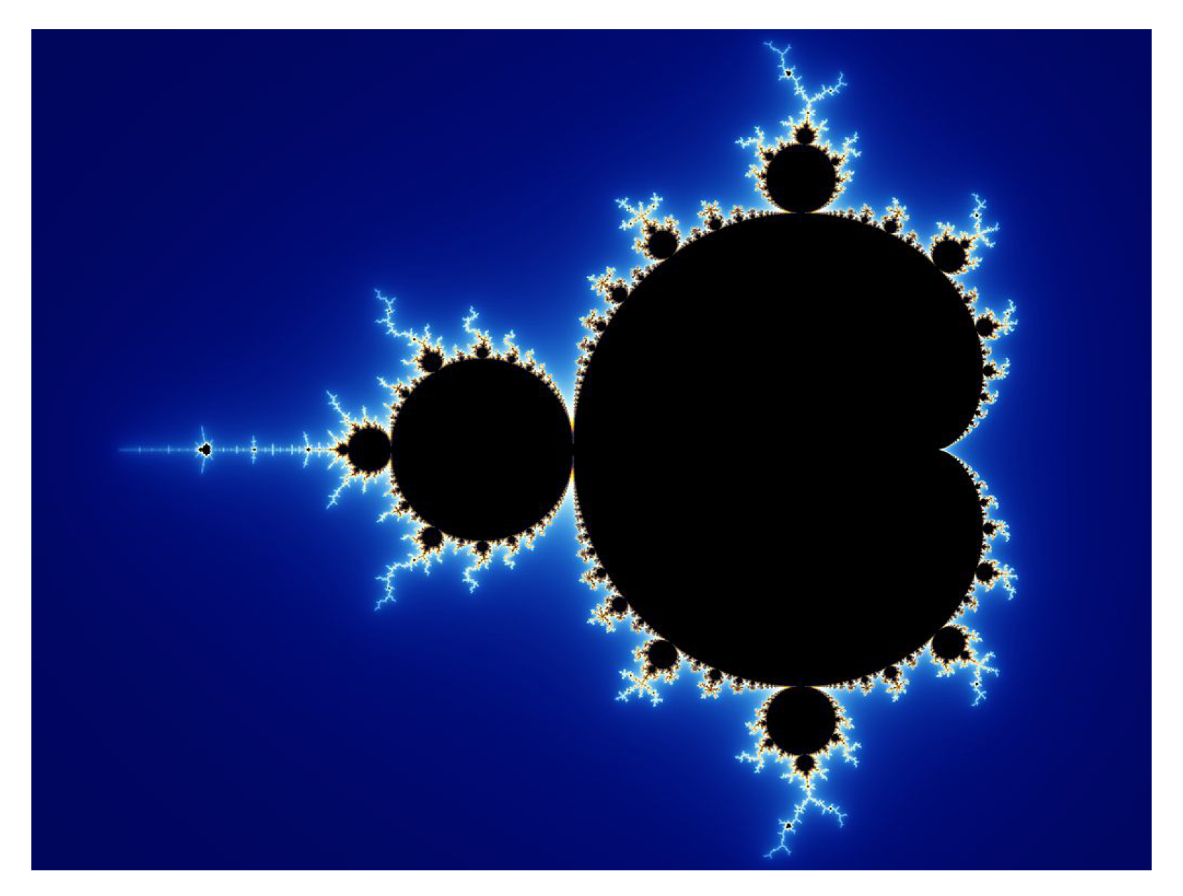
Recurring patterns up to scale similarity are seen in many natural phenomena at all scales. This gives rise to a novel concept of symmetry. This is also known mathematically as a “fractal”, and it occurs when self similarity patterns appear similar at different small scales. For example Mandelbrot set (Figure 5). When a precise and intricate pattern is observed to repeat itself, fractals are employed.

Figure 5. Madelbrot set.

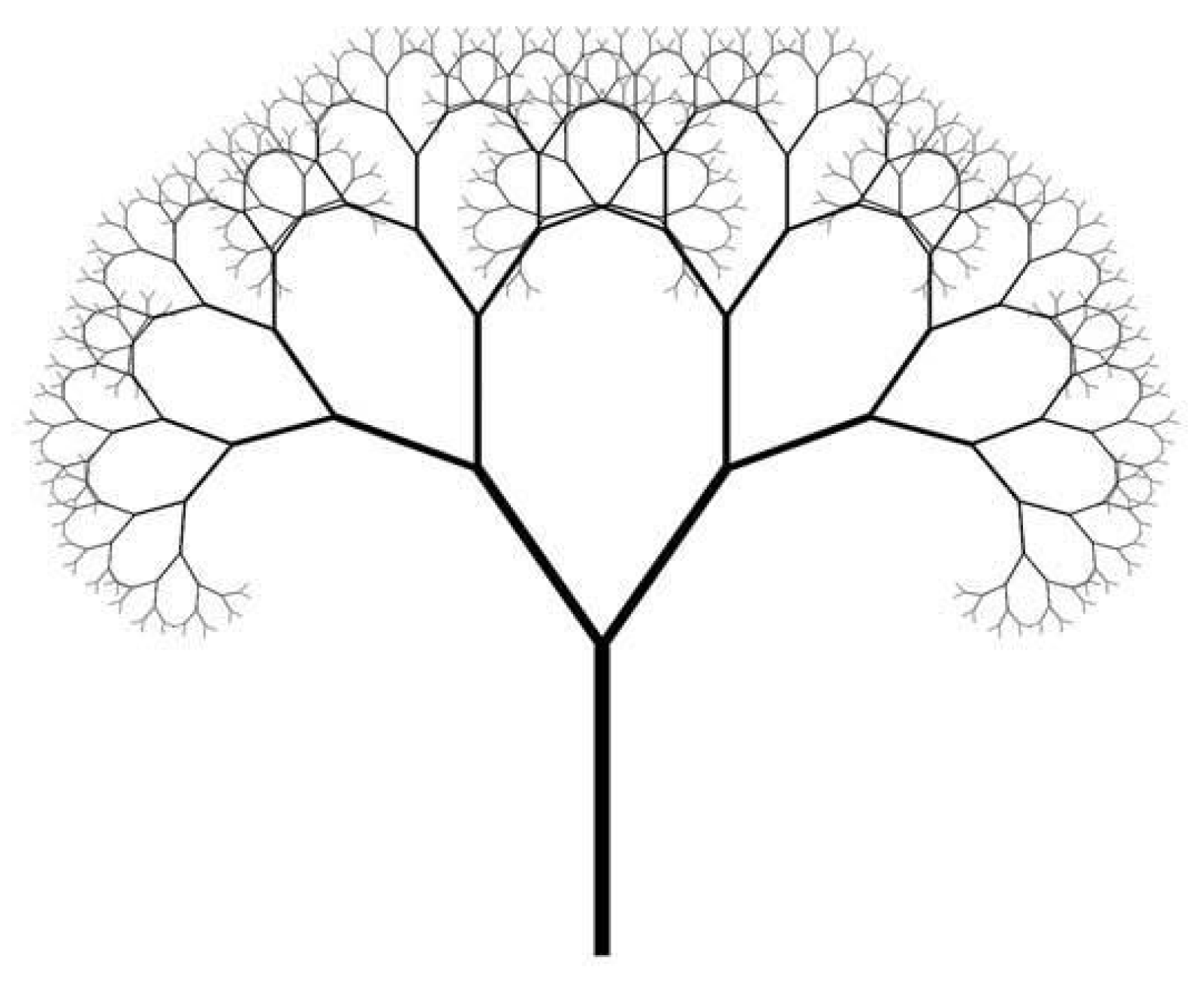
The fractal tree (Figure 6) is another examples of a fractal.

Figure 6. Fractal tree.

Fractal compression uses an image’s self-similarity to its advantage in order to compress data. In this technique, the image is divided into smaller blocks known as range blocks, and comparable patterns inside the image known as domain blocks are found. Fractal compression can achieve high compression ratios by identifying these matches and encoding the modifications required to recreate them.

Now, we give an example to illustrate how fractal compression techniques’ iterative nature helps in measuring distances and similarities between points or patterns within a digital image and is efficient in the compression of an image by repeatedly improving approximations until a near match to the actual image is achieved.

Example 2.

Let $\mathcal{D}={[0,2]}_{\mathbb{Z}}$ be a digital interval with 2-adjacency. Let $X_0$ be a digital image (see Figure 7,

Figure 7. $X_0$.

Using the Ishikawa (16) iteration scheme and ${\eta }_n=0$ and ${\mu }_n=1,n=1,2,3,\dots$, duplicating $X_0$ and attach one copy to the vertex on the lower left and one to the lower right makes a new digital image $X_1$ as (see Figure 8),

Figure 8. $X_1$.

Applying the second iteration on $X_1$, we have again a new digital image $X_2$, which is similar to $X_1$.

$X_2$ (see Figure 9) is therefore the fixed point in this process. We would want to present the mathematical version of the higher process. Give ϝ the function that converts $X_i$ to $\mathsf{𝟊}\left(X_i\right)$. Thus, we can see that $X_2$ is a fixed point of this function or that $\mathsf{𝟊}(X_2)=X_2$. An infinite sequence is produced if the procedure is repeated on $X_n$ sets. There is a convergence of $X_n$ to $X_2$. It is impossible to differentiate between $X_5$ and $X_2$. Consequently, the computer software uses $X_5$ rather than $X_2$ for improved resolution. Simultaneously, the application may quickly determine certain digital image properties by using $X_2$ instead of $X_5$.

Figure 9. $X_2$.

Example 3.

(Sierpinski triangle) We took a triangle and cut off its middle, then we repeated it again to generate the Sierpinski triangle. However, an iterative function system can also be used to represent the Sierpinski triangle. Start with a solid triangle with digital image $I_0$ (see Figure 10).

Figure 10. Generators of Sierpinski triangle.

Then, three functions $\{{\xi }_1,{\xi }_2,{\xi }_3\}$ are generators, representing a contractive mapping are used to form $I_1$. Every mapping reduces the triangle’s size by half, placing the reduced triangles in each of $I_0$’s corners.

The corresponding Iterative process is given by $\{R^2:{\xi }_1,{\xi }_2,{\xi }_3\}$, where the contractive transformations ${\xi }_1,{\xi }_2,$ and ${\xi }_3$ are given by

$$\begin{array}{cc}\hfill {\xi }_1(𝚤,j)& =\left[\begin{array}{cc}\frac{1}{2}& 0\\ 0& \frac{1}{2}\end{array}\right]\left[\begin{array}{c}𝚤\\ j\end{array}\right],\hfill \\ \hfill {\xi }_2(𝚤,j)& =\left[\begin{array}{cc}\frac{1}{2}& 0\\ 0& \frac{1}{2}\end{array}\right]\left[\begin{array}{c}𝚤\\ j\end{array}\right]+\left[\begin{array}{c}\frac{1}{2}\\ 0\end{array}\right],\hfill \\ \hfill x{i}_3(𝚤,j)& =\left[\begin{array}{cc}\frac{1}{2}& 0\\ 0& \frac{1}{2}\end{array}\right]\left[\begin{array}{c}𝚤\\ j\end{array}\right]+\left[\begin{array}{c}\frac{1}{4}\\ \frac{3}{2}\end{array}\right].\hfill \end{array}$$

(27)

The result of this Iterative process is the Sierpinski triangle (see Figure 11) and is given by $I={lim}_{n\to \infty }{\xi }^n\left(I_0\right)$.

Figure 11. Iterations.

4. Conclusions

In conclusion, this paper has undertaken a thorough examination of the advancements achieved in comprehending Iterative Fixed-Point Schemes, grounded in the concept of digital contraction mappings. Additionally, we have introduced the concept of Iterative Fixed-Point Schemes within digital metric spaces. This study extends the Iteration process of Mann (15), Ishikawa (16), Agarwal (17), and Thakur (18), incorporating the $ϝ$-Stable Iterative Scheme in the context of digital metric spaces. The design and exploration of fractal images serve to illustrate the compression of Fixed-Point Iterative Schemes and contractive mappings. Furthermore, a concrete example has been presented to elucidate the underlying motivation for our investigations.

Moreover, our paper has demonstrated the practical application of the proposed Fractal image and Sierpinski triangle in compressing works, specifically addressing the challenge of storing images efficiently by representing them as a collection of digital contractions. This approach offers a solution to the problem of conserving storage memory while retaining the essential features of the images discussed in this study.

References

- Rosenfeld, A. Digital topology. Am. Math. Mon. 1979, 86, 621–630. [Google Scholar] [CrossRef]
- Boxer, L. Remarks on Fixed Point Assertions in Digital Topology, 2. Appl. Gen. Topol. 2019, 20, 155–175. [Google Scholar] [CrossRef]
- Ege, O.K. Some Results on Simplicial Homology Groups of 2D Digital Images. Int. J. Inform. Comput. Sci. 2012, 1, 198–203. [Google Scholar]
- Ege, O.K. Lefschetz Fixed Point Theorem for Digital Images. Fixed Point Theory Appl. 2013, 2013, 253. [Google Scholar] [CrossRef]
- Ege, O.K. Applications of The Lefschetz Number to Digital Images. Bull. Belg. Math. Soc. Simon Stevin 2014, 21, 823–839. [Google Scholar] [CrossRef]
- Ege, O.K. Banach Fixed Point Theorem for Digital Images. J. Nonlinear Sci. Appl. 2015, 8, 237–245. [Google Scholar] [CrossRef]
- Sridevi, K.; Kameswari, M.V.R.; Kiran, D.M.K. Fixed Point Theorems for Digital Contractive Type Mappings in Digital Metric Spaces. Int. J. Math. Trends Technol. (IJMTT) 2017, 48, V48P522. [Google Scholar]
- Boxer, L. A classical construction for the digital fundamental group. J. Math. Imaging Vis. 1999, 10, 51–62. [Google Scholar] [CrossRef]
- Han, S.E. Banach fixed point theorem from the viewpoint of digital topology. J. Nonlinear Sci. Appl. 2015, 9, 895–905. [Google Scholar] [CrossRef]
- Harder, A.M. Hicks, T.L. Stability results for fixed point iteration procedures. Math. J. 1988, 33, 693–706. [Google Scholar]
- Rhoades, B.E. Fixed point theorems and stability results for fixed point iteration procedures II. Indian J. Pure Appl. Math. 1993, 24, 691–703. [Google Scholar]
- Osilike, M.O.; Udomene, A. Short proofs of stability results for fixed point iteration procedures for a class of contractive-type mappings. Indian J. Pure Appl. Math. 1999, 30, 1229–1234. [Google Scholar]
- Zamfirescu, T. Fix point theorems in metric spaces. Arch. Math. 1972, 23, 292–298. [Google Scholar] [CrossRef]
- Berinde, V. On the Stability of Some Fixed Point Procedures. Bul. științific Univ. Baia Mare Ser. Mat. Inform. 2002, XVIII, 7–14. [Google Scholar]
- Berinde, V. On the convergence of the Ishikawa iteration in the class of quasi-contractive operators. Acta Math. Univ. Comen. 2004, LXXIII, 119–126. [Google Scholar]
- Berinde, V. Iterative Approximation of Fixed Points; Springer: Berlin/Heidelberg, Germany, 2007. [Google Scholar]
- Berinde, V. Some remarks on a fixed point theorem for Ciric-type almost contractions. Carpathian J. Math. 2009, 25, 157–162. [Google Scholar]
- Debnath, P.; Torres, D.F.M.; Cho, Y.J. Generalized Boyd-Wong-Type Contractions and Related Fixed-Figure Results. In Advanced Mathematical Analysis and Its Applications; Chapman and Hall/CRC: Boca Raton, FL, USA, 2023; pp. 18–26. [Google Scholar]
- Mann, W.R. Mean value methods in iteration. Proc. Am. Math. Soc. 1953, 44, 506–510. [Google Scholar] [CrossRef]
- Ishikawa, S. Fixed point by a new iteration method. Proc. Am. Math. Soc. 1974, 44, 147–150. [Google Scholar] [CrossRef]
- Agarwal, R.P.; O’Regan, D.; Sahu, D.R. It Fixed Point Theory for Lipschitzian Type Mappings with Applications, Topological Fixed Point Theory and Its Applications; Springer: New York, NY, USA, 2009; Volume 6. [Google Scholar]
- Thakur, B.S.; Thakur, D.; Postolache, M. A new iterative scheme for numerical reckoning fixed points of Suzuki’s generalized nonexpansive mappings. Appl. Math. Comput. 2016, 275, 147–155. [Google Scholar] [CrossRef]
- Botmart, T.; Shaheen, A.; Batool, A.; Etemad, S.; Rezapour, S. A novel scheme of k-step iterations in digital metric spaces. AIMS Math. 2023, 8, 873–886. [Google Scholar] [CrossRef]
Figure 1.
2-adjacent.
Figure 2.
4-adjacent and 8-adjacent.
Figure 3.
6-adjacent, 18-adjacent, and 26-adjacent.
Figure 4.
Graphical presentation of Table 1.
Figure 5.
Madelbrot set.
Figure 6.
Fractal tree.
Figure 7.
.
Figure 8.
Figure 9.
Figure 10.
Generators of Sierpinski triangle.