Multi-Dimensional Data Analysis Platform (MuDAP): A Cognitive Science Data Toolbox

Abstract

Researchers in cognitive science have long been interested in modeling human perception using statistical methods. This requires maneuvers because these multiple dimensional data are always intertwined with complex inner structures. The previous studies in cognitive sciences commonly applied principal component analysis (PCA) to truncate data dimensions when dealing with data with multiple dimensions. This is not necessarily because of its merit in terms of mathematical algorithm, but partly because it is easy to conduct with commonly accessible statistical software. On the other hand, dimension reduction might not be the best analysis when modeling data with no more than 20 dimensions. Using state-of-the-art techniques, researchers in various research disciplines (e.g., computer vision) classified data with more than hundreds of dimensions with neural networks and revealed the inner structure of the data. Therefore, it might be more sophisticated to process human perception data directly with neural networks. In this paper, we introduce the multi-dimensional data analysis platform (MuDAP), a powerful toolbox for data analysis in cognitive science. It utilizes artificial intelligence as well as network analysis, an analysis method that takes advantage of data symmetry. With the graphic user interface, a researcher, with or without previous experience, could analyze multiple dimensional data with great ease.

1. Introduction

The main challenge of cognitive science is not only revealing apparent facts of perception but clarifying the mechanisms behind perception and cognition. However, the researchers examining human cognition are always overwhelmed by the complexity of it. For instance, when perceiving a given face, a viewer is able to extract facial identity, expression, and social characteristics (such as attractiveness and competence) accurately and effortlessly [1,2,3].

The modeling of human perception depends on the repertoire of data analysis methods. A certain number of researchers in cognitive science are only equipped with classical statistical analysis tools such as analysis of variance (ANOVA) and linear regression. These researchers are challenged when studying face perception as many of the dimensions in face perception are intertwined. For instance, facial identity (“Who is the person?”) and facial expression (“What is the emotion?”) are widely believed as distinctive. Facial identity is generally regarded as a kind of invariant information that remains consistent within a short period of time, while facial expression is regarded as kind of variant information that is changeable with even tiny muscle movements from time to time [4,5]. Conversely, the converging evidence suggested that the perceived emotional expression of a face is affected by the facial identity of that person, thus, these two aspects of a face are inter-dependent with each other [6,7]. Similarly, although one may perceive multiple social characteristics from a face, many of these characteristics are heavily correlated with each other [8]. Several past studies like [8,9] even suggested that seemingly complicated social characteristics can be easily represented on a two- or three-dimensional framework. For example, most frameworks believe that the dominance and the trustworthiness of a face are perceived in orthogonal mechanisms.

So far, the researchers in cognitive sciences tend to reduce data dimensions when dealing with face perception data. A common method to conduct dimension-reduction in multiple dimensional data is principal component analysis (PCA), a kind of multivariate method. Briefly speaking, in a typical PCA, the original data matrix (in which data are largely dependent on each other) was transformed into a new matrix formed by the principal components (PCs) calculated via the linear combinations of the original data [10]. The first PC explains most of the data variance, and the following PCs each explain most of the remaining variance. PCA has been widely used in modeling perception of social characteristics, but there are several concerns regarding only using PCA for this kind of multiple dimensional data.

First of all, PCA is not easy to conduct properly. Though some researchers in face perception have used PCA to reduce data dimensions [11,12], the operation procedures of it are not standardized among different labs. In a typical principal component analysis, the original data are supposed to be continuous variables. Whereas, in many human perception studies, the data are measured in discrete Likert scales (e.g., 9 point scale in [8]). Although many treated such data as a kind of continuous variable, some argued this approximation may jeopardize the rigorousness of data analysis. Furthermore, the implications of principal component analysis require maneuvers that many researchers may not actually understand nor even command. For example, the data rotation operation is always recommended but sometimes left undone [8]. In a recent large scaled replication study [13], the authors argued the rotation procedure is vital but has been ignored in some seminal works. Second, PCA is not ideal for all research questions. It operates under the assumption that samples follow some specific distributions, which can lead to meaningless reductions when dealing with data that are not uniformly distributed. For example, real human perception data may contain multiple clusters, but these clusters are not evenly distributed in some unknown dimensions. Furthermore, reducing data dimensions in human perception data is not a necessity. The general logic behind the PCA is to reduce the data dimensions with a mathematical algorithm, but data reduction may not be the omnipotent solution for modeling face perception with a small number of dimensions [14]. Though computer science researchers utilize PCA as well, the number of the output dimensions (the number of PCs) in their typical studies are much greater than the original number of dimensions dealt with in human cognition studies. For example, in one of the pioneer works using computer vision techniques in face perception [15], the authors used 50 PCs to reduce the data dimensions of real face images (with $54,150$ dimensions).

In considering the suitability of PCA as a dimension-reduction technique, t-distributed stochastic neighbor embedding (t-SNE) emerges as an exemplary alternative [16,17]. Notably in its distinction from PCA, t-SNE boasts several advantageous properties. As a nonlinear algorithm, t-SNE excels at preserving the local intricacies of data structures [18,19]. Tailored specifically for visualizing complex, high-dimensional datasets, t-SNE adeptly generates two- or three-dimensional representations that illuminate data clusters and relationships, which may remain obscured by linear methods such as PCA. Furthermore, the robustness of t-SNE for diverse data characteristics sets it apart. It eschews the assumption of a global Gaussian distribution in favor of a more adaptable probabilistic model, capable of flexibly accommodating a spectrum of data distributions. Furthermore, what is worth mentioning is that t-SNE, a projection-based method [20], does not cause serious data loss, so its clustering results on the two-dimensional plane can reveal hidden information that PCA may regard as non-principal components, including new resulting clusters, the internal structure of the data, etc.

To validate the reliability of the data-dimension-reduction results, network analysis, a method that takes advantage of data symmetry is necessary [21,22,23]. Network analysis, especially in the fields of cognition and psychology [24,25,26], is a powerful tool for assessing the reliability of clustering results by leveraging the inherent symmetries within the data. By examining the strength of connections within the network, this method reflects the degree of correlation between clustering results, capitalizing on the symmetry of the pairwise clustering correlation data. By identifying areas where these symmetries hold true, network analysis can confirm that the clustering results are not merely a product of random chance but reflect genuine, underlying groupings within the dataset.

It is challenging and unrealistic for scholars who are not majoring in computer science to use complex dimension-reduction tools, even though in some circumstances, reducing the data dimension is unnecessary. In the sense of this, the neural network approach might be the solution. Using state-of-the-art techniques, the researchers in other research disciplines (specifically, computer vision) classified data with more than hundreds of dimensions with neural networks and revealed the inner structure of the data. This fantastic cutting edge technique has been widely utilized in various applications, such as image classification [27,28,29,30], system identification [31,32,33], natural language processing [34,35,36], autonomous driving [37,38,39,40] and fault diagnosis [41,42,43,44]. Thus, the neural networks might be the ideal candidate to further classify perception data. Although some of the researchers are aware of the neural networks, they have difficulties when applying these techniques. Specifically, it may take a long time to learn the programming language and build the environment for the neural network. Thus, it is reasonable to introduce an easy-to-use platform with a graphic user interface (which is close to much of the statistics software that the researchers used) for the researchers in cognitive science who are not familiar with coding.

Considering the aforementioned concerns, this paper offers the multi-dimensional data analysis platform (MuDAP) for researchers in cognitive science. The MuDAP is designed with a standardized pipeline and equipped with state-of-the-art neural network techniques based on existing machine learning libraries in Python. The contribution of this paper is listed as follows:

• The framework structure of the multi-dimensional data analysis platform (MuDAP) is introduced.
• A graphic visualization data-dimension-reduction algorithm based on t-SNE is utilized to dig the real clusters based on the inner structure of the data.
• A network analysis taking advantage of the symmetric structure of the data on correlations between each predicted cluster is performed to verify the reliability of the clustering results based on the result trustworthiness.
• An embedded neural network training algorithm is proposed to solve the corresponding regression and classification problems using the cluster results as labels.
• A step-by-step illustration of how to use MuDAP, analyzing the introduced face perception experiment data, is shown that verifies the function of the MuDAP.

2. Framework Structure

The multi-dimensional data analysis platform (MuDAP) is built within Python, and its framework structure is first introduced in this section.

2.1. Dataset Import

MuDAP addresses the causal relationship among the class of high dimensional data in cognition science. The imported original data should be obtained from real sconces, such as the decision making or perception collected from a questionnaire survey. In this sense, an element

$${\lambda }_i={[a_1^i\dots a_m^i{l}^i]}^{\top }$$

(1)

denotes a set of collected high dimensional data, where $a_j^i$, $j=1,\dots ,m$ is the value at a featured dimension, m is the total number of element features, and $l^i$ is the labeled value of that element. All these collected elements give rise to the dataset $\mathsf{\Lambda }$ and are, hence, stored in the directory ‘MuPAP/LoadDataFile/…’ with the file name ‘data’ in CSV format.

2.2. Graphic User Interface

As shown Figure A1, MuDAP has a total number of six function buttons in its main welcome screen, and these buttons correspond to the procedures explained below.

1. Dimension Reduction: This function employs the t-SNE method to reduce the high dimensional data to fit a 2D plane and plot all the data with their labels in this plane. It verifies the data structure to confirm if any clusters are formed such that later procedures like regression or classification can be carried out. If so, the users can manually insert the center points of the obtained clusters into the memory.

2. Network Analysis: This function can only be performed after the center points of the clusters are stored. It exploits the relationship between all elements in a cluster and each original featured dimension via network analysis.

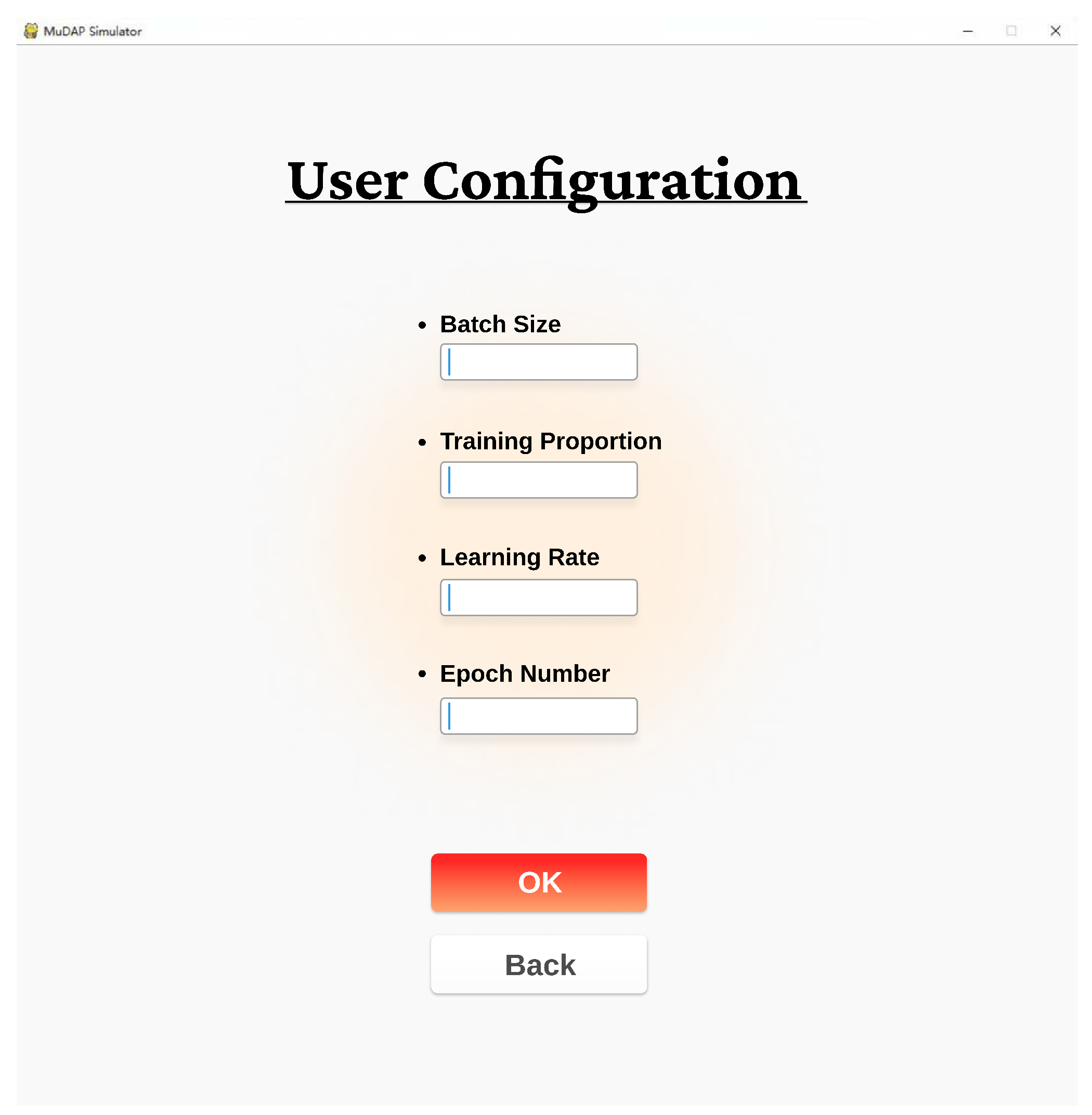
3. User Configuration: This function enables the users to tune the training parameters shown in Figure A2 according to their identical data structure within the later DNN training process.

4. Regression Analysis with DNN: This function trains a deep neural network to predict the distances between any given new element to all existing cluster centers in the 2D plane.

5. Classification Analysis with DNN: This function trains a deep neural network to predict the closest cluster of any given new element in the 2D plane.

6. Contact Information: The developer contact information of MuDAP is shown in this function to allow users to make any direct queries.

The toolbox we have developed operates through a three-step process. Initially, the t-SNE algorithm is utilized to capture the spatial structure of the data without any loss of information. This step is crucial as it provides a comprehensive overview of the data’s inherent dimensions. Second, network analysis is employed to establish direct connections between the various clusters. This analysis is instrumental in validating the relationships within the data and ensuring the reliability of the clustering results. Finally, a neural network is trained to perform regression and classification on the data, which are essential for drawing meaningful insights and predictions. After completing these three steps, the complex and cumbersome high-dimensional cognitive data can be objectively and quantitatively described and analyzed.

2.3. User Instructions for MuDAP

Before conducting any further data analysis, the users must check the data structure of the imported data by using the ‘Dimension Reduction’ function and double check whether the formed clusters have any consistency with the given labels. If there actually exist several clusters, the user can insert the centers into storage and perform the following steps. Then, the ‘Network Analysis’ function is performed to further analyze the relationship between each identical cluster.

After that, the tuning parameters are set in the ‘User Configuration’ function before any neural network training procedures. Hence, the DNN is trained to solve the respective regression and classification problems via the ‘Regression Analysis with DNN’ and ‘Classification Analysis with DNN’ functions. In this sense, MuDAP is capable of discovering the causal relationship between the data structure and data type.

3. Neural-Network-Based Training Procedure Description

This section describes the behind-screen mechanism of MuDAP via explaining how to train the corresponding neural network models for both regression and classification problems.

3.1. Problem Formulation

First of all, if the ‘Dimension Reduction’ function confirms that the imported data structures of the obtained data file appear to have some clusters, the user can enter the center point values of these clusters manually. In this sense, MuDAP is capable of classifying the data type via calculating the distance between an obtained element point and each cluster center in the 2D plane. The input and output of a neural network model is given as

$$\begin{array}{cc}\hfill z^{in}& ={[a_1^i{a}_2^i\dots a_m^i]}^{\top },\hfill \end{array}$$

(2)

$$\begin{array}{cc}\hfill z^{out}& ={[z_1^i{z}_2^i\dots z_n^i]}^{\top },\hfill \end{array}$$

(3)

to denote the imported data features and the obtained results associated with each clusters, so the dimension n denotes the total number of clusters. For each element ${\lambda }_i\in \mathsf{\Lambda }$, the distances ${\tilde{z}}_j^i$, $j=1,\dots ,n$ from its t-SNE plot position to all cluster centers are measured to generate the regression benchmark vector

$${\tilde{z}}_i={[{\tilde{z}}_1^i{\tilde{z}}_2^i\dots {\tilde{z}}_n^i]}^{\top }.$$

(4)

Then, denote the index ${\widehat{l}}^i$ of the cluster with the shortest distance to each t-SNE plot. Using these values, the classification benchmark vector is

$${\widehat{z}}_i={[{\widehat{z}}_1^i{\widehat{z}}_2^i\dots {\widehat{z}}_n^i]}^{\top },$$

(5)

whose elements are defined as

$${\widehat{z}}_j^i=\left\{\begin{array}{c}\begin{array}{cc}\hfill 1& ,j={\widehat{l}}^i,\hfill \\ \hfill 0& ,\mathrm{else}.\hfill \end{array}\end{array}\right.$$

(6)

After defining the above regression and classification benchmark vectors, randomly split the original dataset $\mathsf{\Lambda }$ into a training set ${\mathsf{\Lambda }}_{train}$ and a testing set ${\mathsf{\Lambda }}_{test}$ for later on training procedures with a given proportion. Using the above notations, the corresponding regression and classification problems for high dimensional data are stated as below.

Definition 1.

The  High Dimensional Data Regression Problem   is defined as updating the essential parameters of the neural network iteratively alongside the training epochs based on the data from the training set ${\mathsf{\Lambda }}_{train}$, so that the mean square error loss function

$$\mathcal{L}(z_i,{\tilde{z}}_i)=\frac{1}{n}\parallel z_i-{\tilde{z}}_i\parallel ,$$

(7)

is minimized for all elements in ${\mathsf{\Lambda }}_{train}$.

Definition 2.

The   High Dimensional Data Classification Problem   is defined as updating the essential parameters of the neural network repeatedly alongside the training epochs based on the data from the training set ${\mathsf{\Lambda }}_{train}$, such that the cross entropy loss function

$$\mathcal{L}(z_i,{\widehat{z}}_i)=-\sum _{j=1}^n{\widehat{z}}_{i}log{z}_i\left(j\right),$$

(8)

is minimized for every element in ${\mathsf{\Lambda }}_{train}$.

3.2. Neural Network Structure

MuDAP typically employs neural network models to solve the above-mentioned regression and classification problems in Definitions 1 and 2, and an exemplary neural network model is shown in Figure 1 for a direct view. As seen in this figure, the general structure of the embedded model within MuDAP has m units in its input layer and n units in its output layer, respectively. There are k hidden layers in the dashed red box, and each of them has $r_i$ units in it. The layer-to-layer data transformation is described by

$$z_{i+1}^{in}=W_{i+1}{z}_i^{out},$$

(9)

where $z_i^{out}\in {\mathbb{R}}^{r_i}$ is the i-th layer output, $z_{i+1}^{in}\in {\mathbb{R}}^{r_{i+1}}$ is the $(i+1)$-th layer input, and $W_{i+1}\in {\mathbb{R}}^{r_{i+1}\times r_i}$ is a transfer matrix. Moreover, each unit embeds the activation function $f_{i,j}(·)$ as

$$z^{out}=f_{i,j}\left(z^{in}\right)=\mathrm{RReLU}(z^{in}+b_{i,j}),$$

(10)

where $\mathrm{RReLU}(·)$ is a randomized leaky rectified linear unit function

$$\mathrm{RReLU}\left(x\right)=\left\{\begin{array}{c}\begin{array}{cc}\hfill x& ,x⩾0,\hfill \\ \hfill ax& ,\mathrm{else},\hfill \end{array}\end{array}\right.$$

(11)

and a is a small scalar. The activation function $\mathrm{RReLU}(·)$ contributes to the network model with non-linear properties to approach the non-linear logistics function in practice. The output layer computes the result using

$$z_{k+1}^{out}=\mathrm{RReLU}\left(z_{k+1}^{in}\right),$$

(12)

for the regression problem, and

$$z_{k+1}^{out}=g\left(z_{k+1}^{in}\right),$$

(13)

for the classification problem with $g(·)$ being a softmax function

$$g{\left(x\right)}_i=\frac{e^{x\left(i\right)}}{{\sum }_{j=1}^n{e}^{x\left(j\right)}}.$$

(14)

3.3. A Training Algorithm Description

After generating an appropriate neural network model, the embedded neural network training algorithm shown in Algorithm 1 is proposed to handle the problems in Definitions 1 and 2. This algorithm first divides the training set ${\mathsf{\Lambda }}_{train}$ into a series of batches with an equal number of elements, and it employs all elements in each batch to train the parameters with the neural network model. Any batch size larger than 1 is capable of compensating for the negative effect of a single poor/wrong data sample using the other good data in the same batch.

In addition, the estimation accuracy rates of elements within ${\mathsf{\Lambda }}_{train}$ and ${\mathsf{\Lambda }}_{test}$ are denoted as

$${\varphi }_{train}=\frac{{\sum }_{\lambda \in {\mathsf{\Lambda }}_{train}}{\lambda }^{acc}}{\mathrm{len}\left({\mathsf{\Lambda }}_{train}\right)},{\varphi }_{test}=\frac{{\sum }_{\lambda \in {\mathsf{\Lambda }}_{test}}{\lambda }^{acc}}{\mathrm{len}\left({\mathsf{\Lambda }}_{test}\right)},$$

(15)

and considered the performance index of the classification problem, where the correction number of each element ${\lambda }_i$ is denoted as

$${\lambda }_i^{acc}=\left\{\begin{array}{c}\begin{array}{cc}1,\hfill & argmax{z}_i=l^i,\hfill \\ 0,\hfill & \mathrm{else}.\hfill \end{array}\end{array}\right.$$

(16)

Algorithm 1 The embedded neural network training algorithm.

Input: The dataset $\mathsf{\Lambda }$ with high dimensional data structure, the mean square error loss function (7), the cross entropy loss function (8), initial model parameters $W_i$ and $b_{i,j}$, the training element number $\eta$, the training batch size $n_{batch}$ and the total training epoch number $n_{epoch}$. Output: $W_i$ and $b_{i,j}$ (the model parameters). 1: initialization: Training epoch number set at $i=1$. 2: Split $\eta$ elements of $\mathsf{\Lambda }$ to ${\mathsf{\Lambda }}_{train}$ and the rest to ${\mathsf{\Lambda }}_{test}$ randomly. 3: The $\mathrm{int}(\eta /n_{batch})$ batches form from ${\mathsf{\Lambda }}_{train}$. 4: while$i⩽n_{epoch}$do 5:  for$j⩽\mathrm{int}(\eta /n_{batch})$do 6:   Calculate the summation of (7) or (8) regarding the j-th batch. 7:   Calculate the gradients of $W_i$ and $b_{i,j}$ with respect to the obtained sum. 8:   Conduct adaptive moment estimation (Adam) gradient descent training to update $W_i$ and $b_{i,j}$ using the obtained gradients. 9:  end for 10:   Obtain the estimation accuracy rates of the updated model from the data in ${\mathsf{\Lambda }}_{train}$ and ${\mathsf{\Lambda }}_{test}$. 11:   Set $i=i+1$ to the next training epoch. 12: end while 13: return$W_i$ and $b_{i,j}$ (the updated model parameters).

4. Data Analysis

Here is a step-by-step illustration of using MuDAP. In this case, we analyzed the data from a previous study. We first introduce the experimental design and the data structure, then show how to analyze the data via MuDAP.

4.1. Design Parameter Specifications

To obtain the perception data, a total number of 32 independent participants were asked to make their individual judgments on 40 different faces. In this sense, each participant rated these faces from 1–7 based on 8 common social traits and also expressed their subjective feelings on the corresponding possible academic major, i.e., Science and Engineering or Humanity and Social Science. In addition, the authors denoted 1 for least emotional and 7 for most emotional and asked the participants to rate the perceived emotion of each face between 1–7. Therefore, $32\times 40=1280$ human perception elements were then collected to provide a dataset $\mathsf{\Lambda }$, and each element was denoted as

$${\lambda }_i={[a_i^1{a}_i^2\dots a_i^8,b_i,c_i]}^{\top },$$

(17)

where $a_i^j$, $j=1,\dots ,8$ is the subject perception value on each social traits, $b_i$ is the perceived emotion of that face, and $c_i$ represents the binary feeling concerning academic major. To avoid the subjective interference in decision making, the authors further transferred these values into either 0 or 1 to yield a sparse enough data structure. The data have been kept publicly available at the Open Science Framework (OSF) and can be accessed at https://osf.io/4zf8t/ (accessed on 22 February 2022).

4.2. t-SNE Plot Analysis

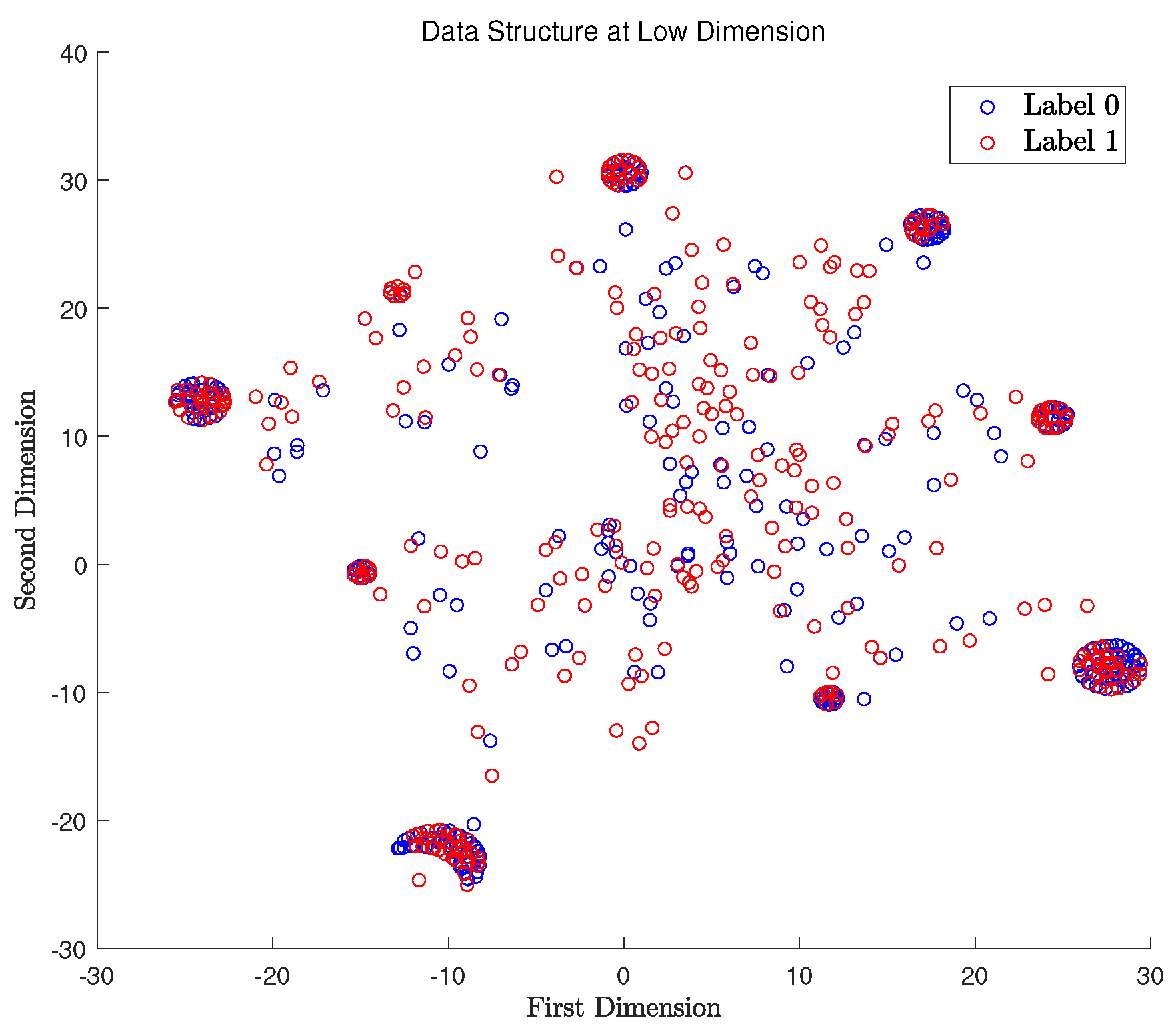
The first step is to examine whether the obtained 8 social trait ratings plus the perceived emotion are capable of determining the perceived academic major of an identical face. To deal with this case, ${[a_i^1{a}_i^2\dots a_i^8,b_i]}^{\top }$ and $c_i$ are treated as a data tuple, as well as a label. The t-SNE method is then utilized to plot the 2D projection of the original high dimensional data on a 2D plane, and the results are shown in Figure 2. It is clear from this figure that the data form nine clusters; however, the corresponding labels are rather random and mixed. A conclusion is made that a neural network cannot be trained to accurately tell the correct subject feelings on academic majors using ${[a_i^1{a}_i^2\dots a_i^8,b_i]}^{\top }$.

Based on the previous model of face perception proposed in [5], the social traits belong to the invariant aspect of the face, while the emotional expression belongs to the variant aspect of the face. To model the face perception in a better way, we would like to elucidate the data structure of ${[a_i^1{a}_i^2\dots a_i^8]}^{\top }$ without the disturbance of the emotion effect (i.e., the variant facial information). Hence, we used the same t-SNE method to model these data (see Figure 3) with $b_i$ as the label to see whether there exists any relationship between the social traits and the perceived emotion of the face. To none of our surprise, there was no relationship between them.

In addition, we further check the data structure of ${[a_i^1{a}_i^2\dots a_i^8,b_i,c_i]}^{\top }$ without applying any labels, whose results are plotted in Figure 4. It is obvious that there were now 12 clusters of data in total, which means the subject feelings certainly extend the potential recognition types for the faces.

To validate if the recorded data have any causal relationships, we, hence, checked the data structure of ${[a_i^1{a}_i^2\dots a_i^8]}^{\top }$ with $a_i^1$ being the label. The obtained results are plotted in Figure 5, and no causal relationship can be observed from the figure. The similar procedures were performed for each value of $a_i^j$, $j=1,\dots ,8$, being the label, but no causal relationship could be found either. Therefore, we have to reach the sad conclusion that the current data do not have any causal relationships between them.

4.3. Perception Data Analysis

For further analysis, we use the results in the above subsection with respect to ${[a_i^1{a}_i^2\dots a_i^9]}^{\top }$. We insert each cluster center into the ‘x-axis’ and ‘y-axis’ textboxes in the ‘Dimension Reduction’ function screen and then click the ‘Add’ button to save the results into memory.

Then, we analyze the relationship between each facial feature and face cluster using the ‘Network Analysis’ function. For each type of face cluster, we count how many $a_i^j$, $j=1,\dots ,8$ and $b_i$ in the exact type have value 1, and the corresponding percentage values are listed in

Table 1. The summary of the MuDAP output. Each data point indicates the percentage of the social characteristic of that type of face. For instance, face Type 1 is not regarded as attractive.

Unit: %	Attractive	Competence	Trustworthy	Dominant	Moral	Masculine	Mature	Social	Expressive
Type 1	0.00	91.76	81.18	0.00	84.71	98.82	83.53	88.24	80.00
Type 2	0.00	87.50	56.25	97.66	67.19	16.41	85.94	73.44	81.25
Type 3	0.00	92.93	100.00	100.00	89.90	100.00	98.99	87.88	100.00
Type 4	29.67	76.37	49.45	97.25	54.95	89.01	79.67	43.96	35.71
Type 5	100.00	97.21	100.00	100.00	98.61	100.00	100.00	100.00	100.00
Type 6	94.41	76.92	65.03	99.30	78.32	51.05	62.24	93.01	55.24
Type 7	100.00	90.22	90.22	0.00	91.30	100.00	83.70	97.83	100.00
Type 8	100.00	82.09	86.57	0.00	86.57	20.90	82.09	97.01	64.18
Type 9	4.06	56.35	62.94	0.51	69.04	4.06	56.85	75.13	60.41

. The results suggest that the perception of the faces can be summarized as nine types in this figure. In this table, each value represents the weight of that social characteristic in that type of face. For instance, the Type 1 face belongs to people who are perceived as not attractive nor dominant but trustworthy, competent, moral, masculine, mature, sociable, and expressive.

Moreover, for each type of personality, we check through each face type to see the corresponding number of ‘1’ for this personality, then divide the sum to obtain the percentage number, and the outputs are listed in

Table 2. The summary of the percentage of (‘1’ at) each facial characteristic involved in each type of observed personality.

Unit: %	Attractive	Competence	Trustworthy	Dominant	Moral	Masculine	Mature	Social	Expressive
Type 1	0.00	7.37	7.08	0.00	7.06	10.00	6.80	7.08	7.11
Type 2	0.00	10.58	7.38	15.04	8.43	2.50	10.54	8.88	10.88
Type 3	0.00	8.69	10.15	11.91	8.73	11.79	9.39	8.22	10.36
Type 4	8.40	13.13	9.23	21.30	9.80	19.29	13.89	7.55	6.80
Type 5	44.63	26.35	29.44	34.54	27.75	34.17	27.49	27.10	30.02
Type 6	21.00	10.39	9.54	17.09	10.98	8.69	8.52	12.56	8.26
Type 7	14.31	7.84	8.51	0.00	8.24	10.95	7.38	8.50	9.62
Type 8	10.42	5.19	5.95	0.00	5.69	1.67	5.27	6.14	4.50
Type 9	1.24	10.48	12.72	0.12	13.33	0.95	10.73	13.98	12.45

. With this table, we are able to qualify to what extent each facial characteristic determines each type of personality. The 5th type of personality encompasses all nine characteristics and is the type that has the high probability. The ‘attractiveness’ largely determines 5th, 6th, 7th and 8th types of personalities; the ‘trustworthiness’ largely determines the 3rd, 5th and 9th ones; the ‘dominance’ largely determines the 2nd, 3rd, 4th, 5th and the 6th ones; the ‘masculinity’ largely determines the 1st, 3rd, 4th, 5th and the 7th ones.

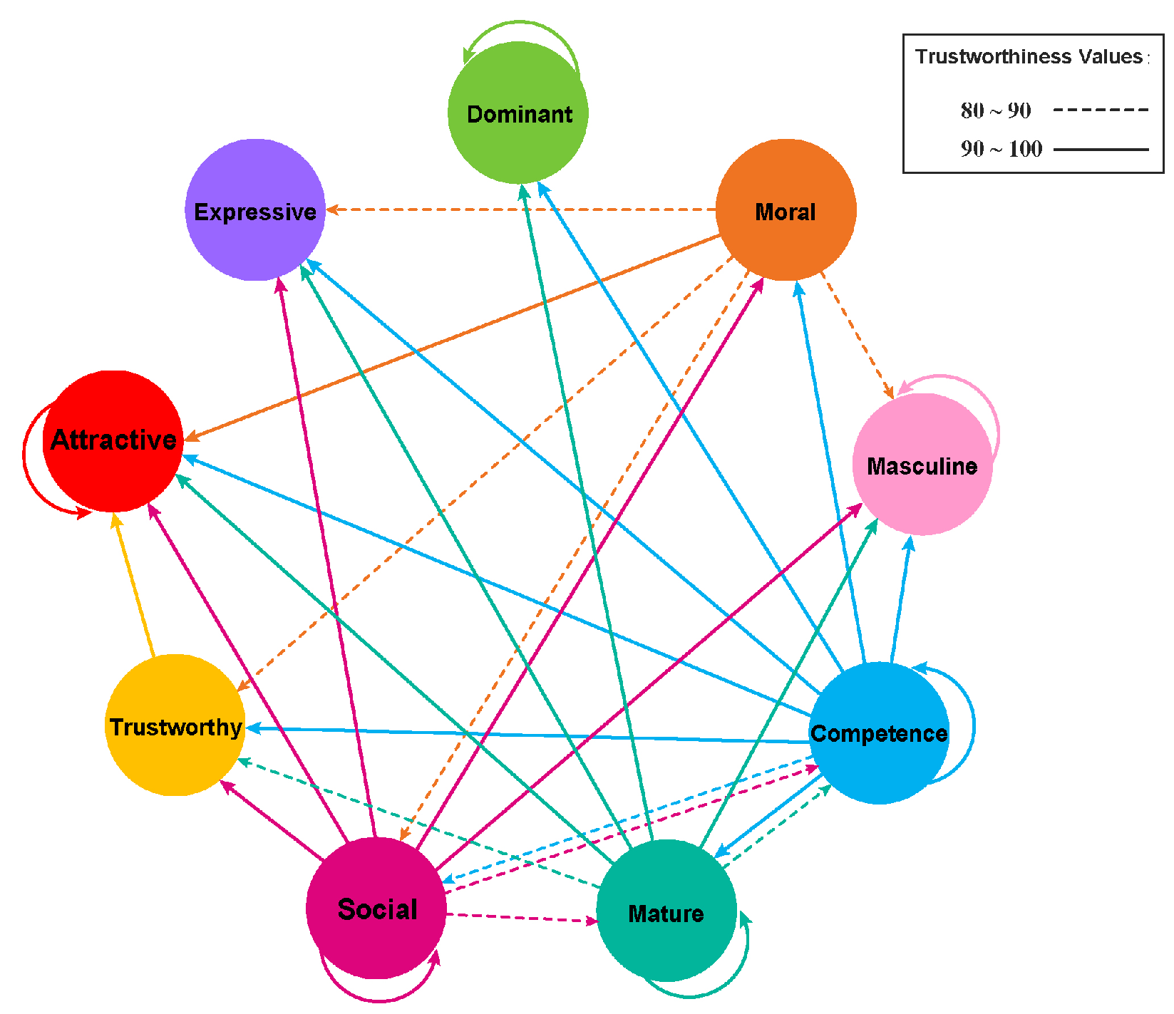
Using the network analysis explained in [24] (with the threshold predetermined by a Sigmoid function), we can better clarify the relationship among the facial characteristics we tested (

Table 3. The outcome matrix of network analysis on 9 observed types of personalities. Each value represents the degree to which one character (row) is predicted by another character (column), e.g., the value $92.90$ indicates that the Type4 is largely determined by Type1.

Unit: %	Attractive	Competence	Trustworthy	Dominant	Moral	Masculine	Mature	Social	Expressive
Attractive	99.70	0.00	0.00	0.00	0.00	0.00	0.00	0.00	0.00
Competence	98.30	92.30	92.80	97.40	90.40	98.70	92.80	89.40	94.80
Trustworthy	92.90	0.00	0.00	0.00	0.00	0.00	0.00	0.00	0.00
Dominant	0.00	0.00	0.00	100.00	0.00	0.00	0.00	0.00	0.00
Moral	98.20	0.00	84.30	0.00	0.00	87.80	0.00	80.10	86.60
Masculine	0.00	0.00	0.00	0.00	0.00	99.00	0.00	0.00	0.00
Mature	94.30	87.60	89.40	97.00	84.00	98.40	90.40	0.00	92.20
Social	99.80	89.40	96.50	0.00	95.20	91.70	87.60	96.90	97.30
Expressive	0.00	0.00	0.00	0.00	0.00	0.00	0.00	0.00	0.00

). First, it is obvious that three characteristics, attractiveness, dominance, and masculinity, are only determined by themselves. This finding is coherent with the theory from [9] (using PCA) that the various facial characteristics are driven by three PCs. The other facial characteristics are more likely to be secondary characteristics, which are driven by the aforementioned three characteristics. Interestingly, the expressiveness, representing the emotional valence, is not driven by any characteristic directly, indicating its uniqueness in face perception compared with other social characteristics. For a visual view, the relationship between the nine features obtained from network analysis is then shown in Figure 6.

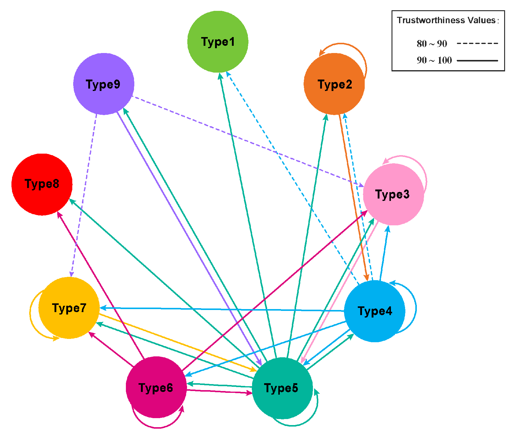
We then applied the same analysis on the relationship among nine observed types of personalities (

Table 4. The outcome matrix of network analysis on 9 facial characteristics. Each value represents the degree to which one character (row) is predicted by another character (column), e.g., the value $92.97$ indicates that the trustworthiness is largely determined by attractiveness.

Unit: %	Type1	Type2	Type3	Type4	Type5	Type6	Type7	Type8	Type9
Type1	0.00	0.00	0.00	0.00	0.00	0.00	0.00	0.00	0.00
Type2	0.00	90.80	0.00	94.07	0.00	0.00	0.00	0.00	0.00
Type3	0.00	0.00	96.55	0.00	97.76	0.00	0.00	0.00	0.00
Type4	89.30	88.57	99.95	96.87	99.99	98.82	98.93	0.00	0.00
Type5	100.00	100.00	100.00	100.00	100.00	100.00	100.00	100.00	100.00
Type6	0.00	0.00	98.92	0.00	99.99	99.40	99.38	93.81	0.00
Type7	0.00	0.00	0.00	0.00	95.27	0.00	91.13	0.00	0.00
Type8	0.00	0.00	0.00	0.00	0.00	0.00	0.00	0.00	0.00
Type9	0.00	0.00	89.79	0.00	95.71	0.00	88.89	0.00	0.00

). The 5th type of personality is linked with all kinds of personalities but the 1st and the 8th ones. Therefore, one may conclude that the 5th type of personality might be the most typical male professor. However, the 1st and the 8th types of personalities do not originate from any kind of personality. Considering the small numbers of these two types, it is possible these two types are simply the collections of undefined personalities. Similarly, the relationships between the nine types obtained from network analysis are illustrated in Figure 7.

4.4. Neural Network Analysis

Based on the clustering results obtained in the previous two subsections, the following two neural-network-based regression and classification tasks will naturally be derived.

The neural network model used in this paper has a total number of five hidden layers, and the numbers of units in these layers are further defined as follows:

$$r_1=64,r_2=128,r_3=64,r_4=32,r_5=16,r_5=9,$$

(18)

respectively. The regression problem is solved using the ‘Regression Analysis with DNN’ function by setting the following configurations

$$n_{batch}=10,n_{epoch}=50,\eta =1,024,\gamma =0.003,$$

(19)

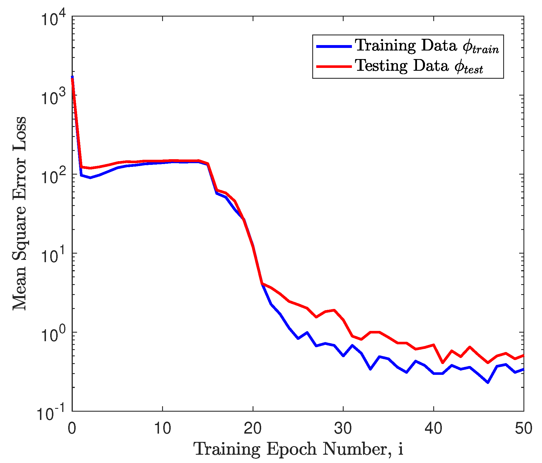
where $\gamma$ is the learning rate of the Adam gradient descent training procedure. The training loss and the testing loss along the time line are shown in Figure 8 with different colors. The mean square training loss declines from over 1000 to below 1, which indicates that the trained neural network accurately predicts the distances between the t-SNE plot of an extra element and the nine cluster centers.

After that, the classification problem is solved using the ‘Classification Analysis with DNN’ function by setting the following configurations:

$$n_{batch}=10,n_{epoch}=100,\eta =1,024,\gamma =0.0003.$$

(20)

The training results are shown in Figure 9 with blue denoting the training accuracy and orange denoting the testing accuracy. The training accuracy rate ${\varphi }_{train}$ rises from the initial value $11\%$ to the final value close to approximately $80\%$ after 100 epochs, and the testing accuracy rate ${\varphi }_{test}$ finally reaches $83\%$. This confirms that the training neural network can accurately predict which cluster is the closest one to the t-SNE plot of an extra element.

With nine social characteristics (or even with fewer PCs), it is mathematically possible to formulate more possible combinations of face type. However, with the DNN analysis, it is obvious that not every combination is possible in real life. This is not practical in classical PCA. In this case, the MuDAP (powered by DNN) is able to illustrate the inner structure of social characteristics and may benefit future research in personality and social traits. For instance, future researchers may study why certain types are formed and why certain combinations do not exist.

5. Conclusions and Future Work

The researchers in cognitive science have long been interested in modeling and classifying the human perception data. This task requires a powerful and easy-to-use analysis platform. Although classical dimension reduction methods like PCA are powerful for building an initial framework, they are not capable of classifying the data and revealing the inner structure and clustering of these data. DNN, on the other hand, has been well-proven to be an ideal method for this kind of research question. However, DNN is not easy to train and implement. Here, the multi-dimensional data analysis platform (MuDAP) with a graphical user interface has been developed to assist cognitive science researchers in handling complex human perception data and classifying its potential structures. The operations of this toolbox are structured into three steps. Initially, dimension reduction based on the t-SNE algorithm captures the spatial structure of the data, identifying nine cluster centers without information loss. Subsequently, network analysis is employed to establish direct connections between each cluster, thereby verifying the reliability of the aforementioned results. Finally, the nine cluster centers are designated as labels, and a neural network is trained to perform both regression and classification on the data. MuDAP facilitates the objective, qualitative, and quantitative analysis of complex, high-dimensional cognitive data, simplifying the research process for cognitive scientists in fields outside of computer science.

In this paper, analyzing the data from the experiment using MuDAP demonstrated that the platform is capable of elucidating the inner structures of various social characteristics (the DNN) and can show the relationship among the different types of personalities (the network analysis). Moreover, using the MuDAP, we are able to show that the facial characteristics of male faces can be summarized in nine types determined mainly by attractiveness, dominance and masculinity but not expressiveness. This finding is inaccessible following dimensional reduction, which only shows the essential components of the social characteristics. Finally, with the help of our trained DNN, new-coming test data are classified into correct clusters, and their distance to each cluster center is predicted accurately.

The MuDAP is an easy-to-use and powerful data analysis platform for cognitive scientists dealing with multiple dimensional data. With this, researchers without expertise in coding can process massive amounts of data with great ease at the GUI. The output of the data offers data classification, which is useful for multiple dimensional data analysis. Therefore, the analysis from the MuDAP complements the usage of the current data analysis methods.

References

- Willis, J.; Todorov, A. First Impressions: Making up your mind after a 100-ms exposure to a face. Psychol. Sci. 2006, 17, 592–598. [Google Scholar] [CrossRef]
- Palermo, R.; Rhodes, G. Are you always on my mind? A review of how face perception and attention interact. Neuropsychologia 2007, 45, 75–92. [Google Scholar] [CrossRef] [PubMed]
- Holmes, A.; Vuilleumier, P.; Eimer, M. The processing of emotional facial expression is gated by spatial attention: Evidence from event-related brain potentials. Cogn. Brain Res. 2003, 16, 174–184. [Google Scholar] [CrossRef]
- Bruce, V.; Young, A. Understanding face recognition. Br. J. Psychol. 1986, 77, 305–327. [Google Scholar] [CrossRef] [PubMed]
- Young, A.W.; Bruce, V. Understanding person perception. Br. J. Psychol. 2011, 102, 959–974. [Google Scholar] [CrossRef]
- Calder, A.J.; Young, A.W. Understanding the recognition of facial identity and facial expression. Nat. Rev. Neurosci. 2005, 6, 641–651. [Google Scholar] [CrossRef]
- Fox, C.J.; Barton, J.J. What is adapted in face adaptation? The neural representations of expression in the human visual system. Brain Res. 2007, 1127, 80–89. [Google Scholar] [CrossRef]
- Oosterhof, N.N.; Todorov, A. The functional basis of face evaluation. Proc. Natl. Acad. Sci. USA 2008, 105, 11087–11092. [Google Scholar] [CrossRef] [PubMed]
- Sutherland, C.A.; Oldmeadow, J.A.; Santos, I.M.; Towler, J.; Burt, D.M.; Young, A.W. Social inferences from faces: Ambient images generate a three-dimensional model. Cognition 2013, 127, 105–118. [Google Scholar] [CrossRef]
- Jolliffe, I.T. Principal component analysis. Technometrics 2003, 45, 276. [Google Scholar] [CrossRef]
- Masulli, P.; Galazka, M.; Eberhard, D.; Åsberg Johnels, J.; Fried, E.I.; McNally, R.J.; Robinaugh, D.J.; Gillberg, C.; Billstedt, E.; Hadjikhani, N.; et al. Data-driven analysis of gaze patterns in face perception: Methodological and clinical contributions. Cortex 2022, 147, 9–23. [Google Scholar] [CrossRef] [PubMed]
- Fysh, M.C.; Trifonova, I.V.; Allen, J.; McCall, C.; Burton, A.M.; Bindemann, M. Avatars with faces of real people: A construction method for scientific experiments in virtual reality. Behav. Res. Methods 2022, 54, 1461–1475. [Google Scholar] [CrossRef]
- Jones, B.C.; DeBruine, L.M.; Flake, J.K.; Liuzza, M.T.; Antfolk, J.; Arinze, N.C.; Ndukaihe, I.L.; Bloxsom, N.G.; Lewis, S.C.; Foroni, F.; et al. To which world regions does the valence-dominance model of social perception apply? Nat. Hum. Behav. 2021, 5, 159–169. [Google Scholar] [CrossRef] [PubMed]
- Chang, J.; Lan, Z.; Cheng, C.; Wei, Y. Data Uncertainty Learning in Face Recognition. In Proceedings of the IEEE/CVF Conference on Computer Vision and Pattern Recognition (CVPR), Seattle, WA, USA, 13–19 June 2020; pp. 5710–5719. [Google Scholar]
- Calder, A.J.; Burton, A.; Miller, P.; Young, A.W.; Akamatsu, S. A principal component analysis of facial expressions. Vis. Res. 2001, 41, 1179–1208. [Google Scholar] [CrossRef] [PubMed]
- Gisbrecht, A.; Schulz, A.; Hammer, B. Parametric nonlinear dimensionality reduction using kernel t-SNE. Neurocomputing 2015, 147, 71–82. [Google Scholar] [CrossRef]
- Cai, T.T.; Ma, R. Theoretical Foundations of t-SNE for Visualizing High-Dimensional Clustered Data. J. Mach. Learn. Res. 2022, 23, 1–54. [Google Scholar]
- Hajibabaee, P.; Pourkamali-Anaraki, F.; Hariri-Ardebili, M.A. An Empirical Evaluation of the t-SNE Algorithm for Data Visualization in Structural Engineering. In Proceedings of the 2021 20th IEEE International Conference on Machine Learning and Applications (ICMLA), Pasadena, CA, USA, 13–15 December 2021; pp. 1674–1680. [Google Scholar]
- Alshazly, H.; Linse, C.; Barth, E.; Martinetz, T. Handcrafted versus CNN Features for Ear Recognition. Symmetry 2019, 11, 1493. [Google Scholar] [CrossRef]
- Chatzimparmpas, A.; Martins, R.M.; Kerren, A. t-viSNE: Interactive Assessment and Interpretation of t-SNE Projections. IEEE Trans. Vis. Comput. Graph. 2020, 26, 2696–2714. [Google Scholar] [CrossRef] [PubMed]
- Fried, E.; von Stockert, S.; Haslbeck, J.; Lamers, F.; Schoevers, R.; Penninx, B. Using network analysis to examine links between individual depressive symptoms, inflammatory markers, and covariates. Psychol. Med. 2022, 50, 2682–2690. [Google Scholar] [CrossRef]
- Yan, L.; Wang, Y. The application of multivariate data chain network in the design of innovation and entrepreneurship teaching and learning in colleges and universities. Appl. Math. Nonlinear Sci. 2024, 9. [Google Scholar] [CrossRef]
- Hao, X.; Liu, Y.; Pei, L.; Li, W.; Du, Y. Atmospheric Temperature Prediction Based on a BiLSTM-Attention Model. Symmetry 2022, 14, 2470. [Google Scholar] [CrossRef]
- Borsboom, D.; Deserno, M.K.; Rhemtulla, M.; Epskamp, S.; Fried, E.I.; McNally, R.J.; Robinaugh, D.J.; Perugini, M.; Dalege, J.; Costantini, G.; et al. Network analysis of multivariate data in psychological science. Nat. Rev. Methods Prim. 2021, 1, 58. [Google Scholar] [CrossRef]
- Bahrami, M.; Laurienti, P.J.; Shappell, H.M.; Simpson, S.L. Brain Network Analysis: A Review on Multivariate Analytical Methods. Brain Connect. 2023, 13, 64–79. [Google Scholar] [CrossRef]
- Wang, Y.; Chen, C.; Chen, W. Nonlinear directed information flow estimation for fNIRS brain network analysis based on the modified multivariate transfer entropy. Biomed. Signal Process. Control. 2022, 74, 103422. [Google Scholar] [CrossRef]
- Ning, X.; Tian, W.; He, F.; Bai, X.; Sun, L.; Li, W. Hyper-sausage coverage function neuron model and learning algorithm for image classification. Pattern Recognit. 2023, 136, 109216. [Google Scholar] [CrossRef]
- Liu, S.; Wang, L.; Yue, W. An efficient medical image classification network based on multi-branch CNN, token grouping Transformer and mixer MLP. Appl. Soft Comput. 2024, 153, 111323. [Google Scholar] [CrossRef]
- Wu, X.; Feng, Y.; Xu, H.; Lin, Z.; Chen, T.; Li, S.; Qiu, S.; Liu, Q.; Ma, Y.; Zhang, S. CTransCNN: Combining transformer and CNN in multilabel medical image classification. Knowl. Based Syst. 2023, 281, 111030. [Google Scholar] [CrossRef]
- Ma, P.; He, X.; Liu, Y.; Chen, Y. ISOD: Improved small object detection based on extended scale feature pyramid network. Vis. Comput. 2024. early access. [Google Scholar] [CrossRef]
- Wang, G.; Zhang, F.; Chen, Y.; Weng, G.; Chen, H. An active contour model based on local pre-piecewise fitting bias corrections for fast and accurate segmentation. IEEE Trans. Instrum. Meas. 2023, 72, 5006413. [Google Scholar] [CrossRef]
- Wang, L.; Huangfu, Z.; Li, R.; Wen, X.; Sun, Y.; Chen, Y. Iterative learning control with parameter estimation for non-repetitive time-varying systems. J. Frankl. Inst. 2024, 361, 1455–1466. [Google Scholar] [CrossRef]
- Yang, C.; Wu, L.; Chen, Y.; Wang, G.; Weng, G. An Active Contour Model Based on Retinex and Pre-Fitting Reflectance for Fast Image Segmentation. Symmetry 2022, 14, 2343. [Google Scholar] [CrossRef]
- Mikolov, T.; Sutskever, I.; Chen, K.; Corrado, G.S.; Dean, J. Distributed representations of words and phrases and their compositionality. In Proceedings of the 2013 International Conference on Neural Information Processing Systems (NIPS), Lake Tahoe, NV, USA, 5–10 December 2013; pp. 3111–3119. [Google Scholar]
- Gridach, M. A framework based on (probabilistic) soft logic and neural network for NLP. Appl. Soft Comput. 2020, 93, 106232. [Google Scholar] [CrossRef]
- Trinh, T.T.Q.; Chung, Y.C.; Kuo, R. A domain adaptation approach for resume classification using graph attention networks and natural language processing. Knowl. Based Syst. 2023, 266, 110364. [Google Scholar] [CrossRef]
- Wang, L.; Song, Z.; Zhang, X.; Wang, C.; Zhang, G.; Zhu, L.; Li, J.; Liu, H. SAT-GCN: Self-attention graph convolutional network-based 3D object detection for autonomous driving. Knowl. Based Syst. 2023, 259, 110080. [Google Scholar] [CrossRef]
- Chen, Y.; Cheng, C.; Zhang, Y.; Li, X.; Sun, L. A neural network-Based navigation approach for autonomous mobile robot systems. Appl. Sci. 2022, 12, 7796. [Google Scholar] [CrossRef]
- Cheng, C.; Duan, S.; He, H.; Li, X.; Chen, Y. A generalized robot navigation analysis platform (RoNAP) with visual results using multiple navigation algorithms. Sensors 2022, 23, 9036. [Google Scholar] [CrossRef] [PubMed]
- Cui, S.; Chen, Y.; Li, X. A robust and efficient UAV path planning approach for tracking agile targets in complex environments. Machines 2022, 10, 931. [Google Scholar] [CrossRef]
- Chen, Y.; Wu, L.; Wang, G.; He, H.; Weng, G.; Chen, H. An active contour model for image segmentation using morphology and nonlinear poisson’s equation. Optik 2023, 287, 170997. [Google Scholar] [CrossRef]
- Zhao, Z.; Wang, J.; Tao, Q.; Li, A.; Chen, Y. An unknown wafer surface defect detection approach based on Incremental Learning for reliability analysis. Reliab. Eng. Syst. Saf. 2024, 244, 109966. [Google Scholar] [CrossRef]
- Wen, C.; Xue, Y.; Liu, W.; Chen, G.; Liu, X. Bearing fault diagnosis via fusing small samples and training multi-state siamese neural networks. Neurocomputing 2024, 576, 127355. [Google Scholar] [CrossRef]
- Liang, P.; Deng, C.; Yuan, X.; Zhang, L. A deep capsule neural network with data augmentation generative adversarial networks for single and simultaneous fault diagnosis of wind turbine gearbox. ISA Trans. 2023, 135, 462–475. [Google Scholar] [CrossRef]
Figure 1.
The structure of the embedded neural network model.
Figure 2.
2D plot of with marked label using t-SNE.
Figure 3.
Figure 4.
2D plot of without any marked labels using t-SNE.
Figure 5.
Figure 6.
The visual view of the relationship between the 9 features using network analysis, where solid lines are values 90–100, dashed lines are for values 80–90, and arrows are the pointing directions.
Figure 7.
The visual view of the relationship between the 9 types using network analysis, where solid lines are for values 90–100, dashed lines are for values 80–90, and arrows are the pointing directions.
Figure 8.
The training results of the neural network for the regression problem.
Figure 9.
The training results of the neural network for the classification problem.