Article

Computing the Surface Area of Three-Dimensional Scanned Human Data

1
Department of Multimedia Engineering, Dongguk University, Seoul 04620, Korea
2
Department of Computer Engineering, Chosun University, Gwangju 61452, Korea
*
Author to whom correspondence should be addressed.
Current address: Department of Computer Engineering, Chosun University, 309 Pimun-daero, Dong-gu, Gwangju 61452, Korea
Symmetry 2016, 8(7), 67; https://doi.org/10.3390/sym8070067
Submission received: 16 March 2016 / Revised: 22 June 2016 / Accepted: 13 July 2016 / Published: 20 July 2016
(This article belongs to the Special Issue Symmetry in Complex Networks II)

Abstract

:
An efficient surface area evaluation method is introduced by using smooth surface reconstruction for three-dimensional scanned human body data. Surface area evaluations for various body parts are compared with the results from the traditional alginate-based method, and quite high similarity between the two results is obtained. We expect that our surface area evaluation method can be an alternative to measuring surface area by the cumbersome alginate method.

Graphical Abstract

1. Introduction

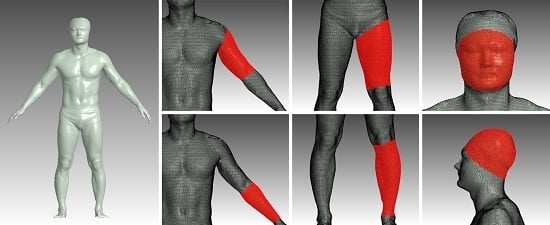
The surface area of human body parts provides important information in medical and medicinal fields, and surface area computation of human body parts is generally a difficult problem. For example, we need to know the accurate surface area when we have to determine the adequate amount of ointment to apply. So far, alginate [1] is generally used to measure surface area. The surface areas of body parts are modeled with alginate, and the models are cut into small pieces. These pieces are spread onto a two-dimensional (2D) plane, and their areas are then measured on the plane, and the total area of the surface is computed by summing the areas of all the pieces. Figure 1 illustrates the overall process for measuring surface area by using alginate. Error is inevitably included in the process of projecting a three-dimensional (3D) surface onto a 2D plane. Moreover, errors by human operators can also accumulate in this process since it requires numerous manual operations.
Recently, the rapid advances in 3D shape scanning technology have enabled us to easily obtain geometric information of real 3D models. Three-dimensional shapes from 3D scanners are already used in ergonomic design, e.g., in the garment, furniture, and automobile industries, as well as in the digital content industry such as movies and animations. In this paper, we further extend the usage of 3D scanned human data to medical and medicinal fields. It would be quite useful to utilize 3D scanned human data to avoid the onerousness of the alginate method.
Three-dimensional scanners usually generate polygonal approximation to human model, and its polygon areas are summed to compute the desired surface area. However, this discrete method does not consider the smooth surface property of human skin and the resulting surface area tends to be smaller than the exact one. We prove this fact with some geometric objects whose exact area values are known. Furthermore, we propose an effective area computation method to overcome the limitation of the polygonal approximation. We reconstruct a smooth surface from the polygonal approximation to reflect the smooth surface property of human body parts, thus reducing the error of area measurement. A local part of the scanned data is selected by a user and reconstructed as a smooth surface; the surface area is then accurately computed by using an analytic method.
We compared the surface areas measured by our method with the ones obtained by using alginate. We set up 15 local parts of a human body, and we measured the areas of the local parts of eight people by using alginate. Three-dimensional human models of the same eight people were also generated by 3D scanning. We selected 15 local parts of the 3D models using an intuitive sketch-based user interface that we developed. We reconstructed smooth surfaces for the selected parts and computed the surface areas from the reconstructed surfaces. We analyzes the similarity and the correlation between the area measured by using alginate and the area computed from our reconstruction method, and found a similarity of >95%. Therefore, we expect that our surface area measuring method can be an effective alternative to measuring surface area, replacing the cumbersome alginate method.
The main contributions of this paper can be summarized as follows:
  • We propose a simple and effective area computation method based on surface reconstruction for the body parts of 3D scanned human models.
  • The area computed using the surface reconstruction method has a 95% similarity with that obtained by using the traditional alginate method.
  • Our area computation method proves to be a possible substitute for the cumbersome alginate method.
The rest of this paper is organized as follows. In Section 2 we briefly review some related recent work on scanning technology and surface reconstruction, and in Section 3 we explain how to reconstruct a smooth surface from polygonal meshes and how to compute the surface area from the reconstructed surfaces. In Section 4 we compare the surface areas of various body parts measured by our method with ones obtained by using the traditional alginate method and derive statistical information. In Section 5 we conclude the paper and suggest some future research.

2. Related Work

Recent advances in 3D scanning technology have made it quite easy to achieve 3D shapes of complex objects. Depending on the specific sensors such as lasers, patten lights, optical cameras, and depth cameras, various types of 3D scanners have been developed. In general, 3D scanners can be classified into three types [2]: Contact types, non-contact active types, and non-contact passive types. Contact 3D scanners contact an object with a tiny, thin needle-like sensor and scan the surface of the object. They can scan the front side of the object, but they hardly scan the side portions or concave parts. Non-contact active 3D scanners use a laser to illuminate the object surface to measure the distances or to recognize surficial curves. Non-contact passive 3D scanners use reflective visible light or infrared light from the object to scan the surface of the object, instead of using laser light or sonic waves.
Depending on the specific application, different types of 3D scanners can be used. For example, whole-body 3D scanners [3,4] are widely used for ergonomic design in the garment, furniture, and automobile industries. These whole-body 3D scanners are equipped with four wide-view, high-resolution scanners, which rotate around the person to scan every angle. This high-powered precision scan is able to capture even the smallest details, such as hair, wrinkles on clothes, and buttons. The scanning process generates millions of triangulated surfaces, which are automatically merged and stitched together. A hand-held 3D scanner is similar to a video camera but captures in three dimensions. It is extremely portable and can be used for medical and biomechanical research. For example, portable oral scanners [5,6] are essential for implant surgical guidance and prosthetic design in dentistry.
Even though 3D scanners provide accurate and detailed geometric data from real-world objects, they are restricted to producing a discrete representation such as unorganized point clouds or polygonal meshes. Moreover, these models can have serious problems for many practical applications; these include irregularity, discontinuity, huge dataset size, and missing areas.
Body surface area (BSA) represents the whole area of a human body, and it is an important quantity in the fields of medicine, pharmacy, and ergonomics. Direct BSA measurement uses paper wrapping, bandage, alginate method and so on, but it is very burdensome work. BSA estimation formula is generally determined by one’s height and weight, and many efforts have been made to find more accurate estimation. Recently, new BSA estimation formulas have been proposed by using 3D scanned human data [7,8,9]. Lee and Choi [10] compared alginate method and 3D body scanning in measuring BSA. They reported that BSA measured by the 3D scanning method tended to be smaller than that by the alginate method.
In this paper, we aim to measure the surface area of a selected region of 3D scanned human data. Summing the polygonal area of the selected region can be one of the simplest ways of measuring surface area. However, we take a different approach to obtain a more accurate result than from a polygonal approximation. We reconstruct a smooth surface from the selected region and compute its surface area based on analytic methods rather than on a simple polygonal approximation. Since smooth surface reconstruction is highly important in our method, we briefly review the related techniques for reconstructing a smooth surface from a polygonal mesh.
Vlachos et al. [11] introduced point-normal (PN) triangles for surfacing a triangular mesh. On each triangle of a mesh, they created a cubic Bézier triangle using vertices and normals from the mesh. However, this method is restricted to generating a G 0 -continuous surface across the triangle boundaries, which is not suitable for measuring surface area.
Blending techniques are widely used for reconstructing a smooth surface in geometric modeling. Vida et al. [12] surveyed the parametric blending of curves and surfaces. Depending on the number of surfaces to be blended, various approaches have been proposed. Choi and Ju [13] used a rolling ball to generate a tubular surface with G 1 -continuous contact to the adjacent surfaces. This technique can be made more flexible by varying the radius of the ball [14]. Hartmann [15] showed how to generate G n parametric blending surfaces by specifying a blending region on each surface to be blended, and reparameterizing the region with common parameters. A univariate blending function is then defined using one of three common parameters to create a smooth surface. This method was extended to re-parameterize the blending regions automatically in [16].
A more general blending scheme was introduced by Grim and Hughes [17]. They derived manifold structures such as charts and transition functions from a control mesh and reconstructed a smooth surface by blending geometries on overlapping charts using a blending function. Cotrina and Pla [18] generalized this method to construct C k -continuous surfaces with B-spline boundary curves. This approach was subsequently generalized by Cotrina et al. [19] to produce three different types of surfaces. However, these techniques require complicated transition functions between overlapping charts.
Ying and Zorin [20] created smooth surfaces of arbitrary topology using charts and simple transition functions on the complex plane. This approach provides both C continuity and local control of the surface. However, the resulting surfaces are not piecewise polynomial or rational. Recently, Yoon [21] extended this technique to reconstruct a smooth surface using displacement functions. Compared to other methods [20,22,23], this method produces a smooth surface that interpolates the vertices of a control mesh, which is an essential condition for measuring the surface area from a smooth surface rather than a polygonal mesh. Therefore, we employ this method to reconstruct a smooth surface and measure its surface area.

3. Computing the Surface Area of 3D Scanned Human Data

In this section we propose a method for computing the surface area of 3D scanned human data. We reconstruct a smooth surface representing the selected region of 3D scanned human data. We then compute the surface area of the selected region from the smooth surface rather than from the triangular mesh, which gives us more accurate results.

3.1. Natural User Interface for Selecting the Region of Interest

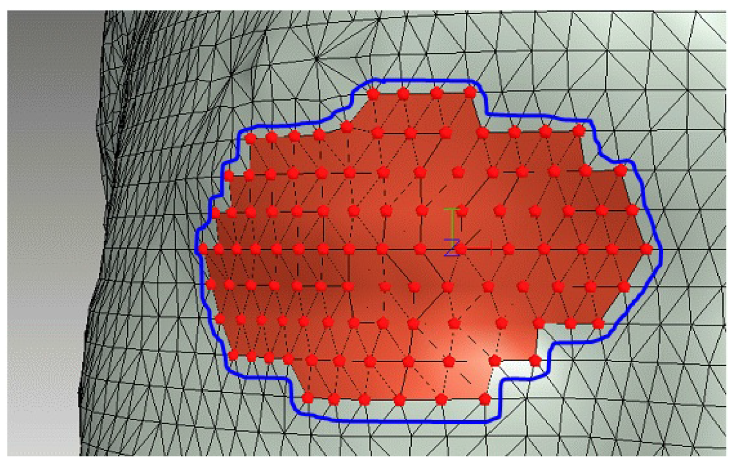
Our system provides a user with a sketch-based interface for specifying the region on the 3D scanned human data. A user marks a closed curve on a 2D screen using the sketch interface. We determine the screen coordinates of the vertices of 3D human data using a graphics pipeline and select only vertices with coordinates inside the marked curve [24]. Figure 2 shows a selected region of 3D human data using the sketch-based user interface.

3.2. Smooth Surface Reconstruction

We employ a method proposed by Yoon [21] to reconstruct a smooth surface from the selected region of 3D human data. This section briefly introduces how to reconstruct a smooth surface for the selected region.
Chart and transition function: For each vertex of the selected region, we define a chart in the 2D complex plane. The chart shape is determined by the degree of a vertex. Figure 3 shows the charts U i and U j of two vertices with different degrees 6 and 3, respectively. As shown in Figure 3, adjacent charts share two regions and their correspondence is defined by a transition function θ i j ( z ) as follows:
z = θ i j ( z ) = z k i / k j ,
where k i and k j represent the degrees of vertices v i and v j , respectively. For instance, let z = u + i v = ( u , v ) be the coordinates of z in the chart U i , then the corresponding coordinates z in U j can be computed by z = z 6 / 3 in Figure 3. For more information, refer to [21].
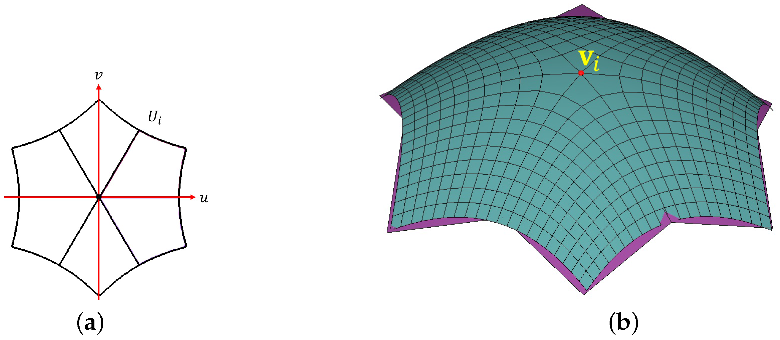
Local Surface Patches: For each chart U i of a vertex v i , we construct a 3D surface patch P i ( u , v ) approximating the 1-ring neighborhood of v i . We employ a biquadratic surface patch P i ( u , v ) defined as follows:
P i ( u , v ) = 1 u u 2 c 1 c 2 c 3 c 4 c 5 c 6 c 7 c 8 c 9 1 v v 2 ,
where c 1 is set to v i for P i ( 0 , 0 ) = v i and other coefficient vectors are determined by approximating 1-ring neighboring vertices of v i in a least-squares sense. Figure 4 shows a local surface patch P i ( u , v ) of v i defined on chart U i .
Blending Surface: We reconstruct a smooth surface by blending the local surface patches. For this, we need a blending function w i ( u , v ) on each chart U i . To construct a blending function w i ( u , v ) , we first construct a piece of blending function η ( u ) η ( v ) on the unit square [ 0 , 1 ] × [ 0 , 1 ] , where η ( t ) = 2 t 3 3 t 2 + 1 . We then apply conformal mapping to η ( u ) η ( v ) , followed by rotating and copying. Figure 5 shows the example of a blending function w i ( u , v ) on a chart of degree k = 6 . Note that blending functions w i ( u , v ) satisfy the partition of unit, i w i ( u , v ) = 1 , on overlapping charts.
Finally, our blending surface S i ( u , v ) on a chart U i is defined by a weighted blending of local patches P j as follows:
S i ( u , v ) = j I z w j θ i j ( z ) P j θ i j ( z ) ,
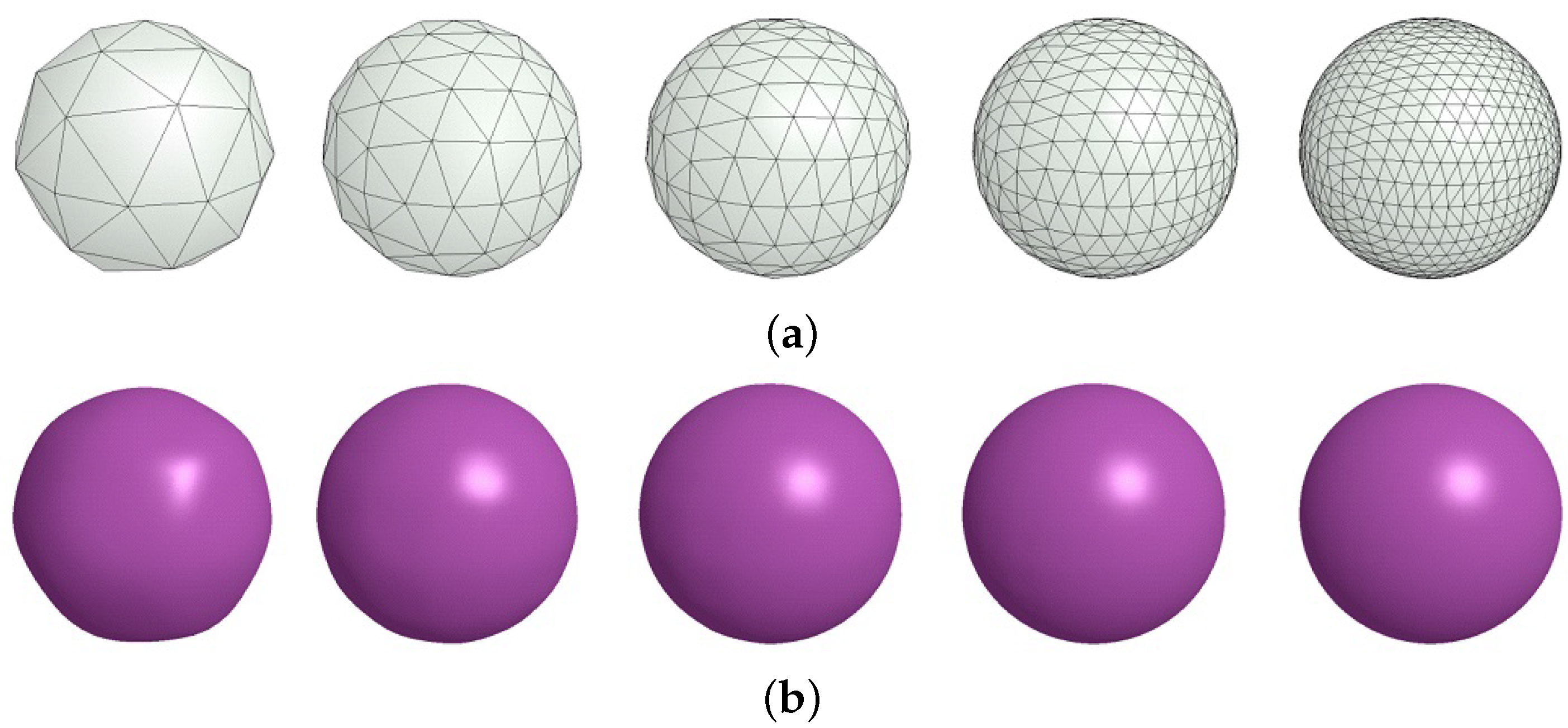
where I z is a set of chart indices containing z = ( u , v ) . Figure 6a shows polygon meshes of different resolutions, generated from a sphere of radius = 5 cm and Figure 6b shows the corresponding blending surfaces generated by using our method.
Measuring Surface Area: Now we can measure the surface area on a smooth blending surface rather than a polygon mesh as follows:
A = | I | d u d v ,
where | I | is the determinant of the first fundamental form matrix [25]. In general, a polygon mesh generates a surface area smaller than that of a smooth surface. To compare and analyze the accuracy of the proposed method, we measure the surface areas of three geometric objects with different distributions of Gaussian curvature. All 3D shapes, including a human body, can locally be classified into the following cases in terms of Gaussian curvature distributions.
Our first example is a sphere with positive Gaussian curvature ( K > 0 ) everywhere. Figure 6a,b show the polygon spheres with the different resolutions and the reconstructed smooth surfaces, respectively. Table 1 compares two surface areas of polygon meshes and reconstructed surfaces in Figure 6. The third column lists the surface areas and computation times measured from polygon meshes and the fourth column lists those from reconstructed surfaces. The next two columns show errors between measured areas and the exact one ( π 314 . 15926535897 ), and their ratios are shown in the last column.
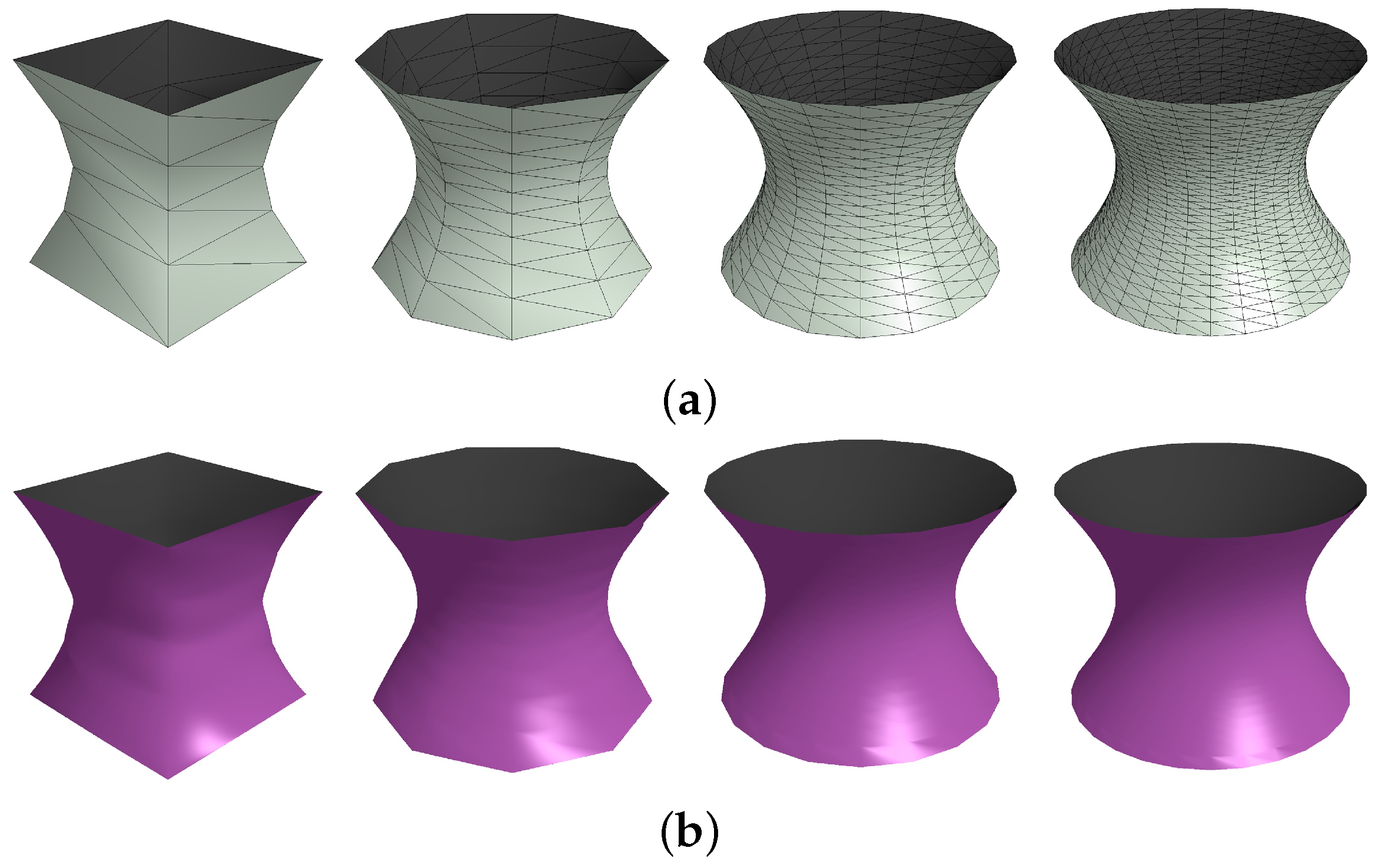
We employ a hyperboloid as the second example, which has negative Gaussian curvature ( K < 0 ) everywhere. Figure 7a,b show the polygon approximations to a hyperboloid with different resolutions and the reconstructed smooth surfaces, respectively. Table 2 compares two surface areas of polygon meshes and reconstructed surfaces in Figure 7. The third column lists the surface areas and computation times measured from polygon meshes and the fourth column lists those from the reconstructed surfaces. The next two columns show errors between measured areas and the exact one ( π ( 2 6 + 2 sinh 1 ( 2 ) ) 20 . 01532 ), and their ratios are shown in the last column.
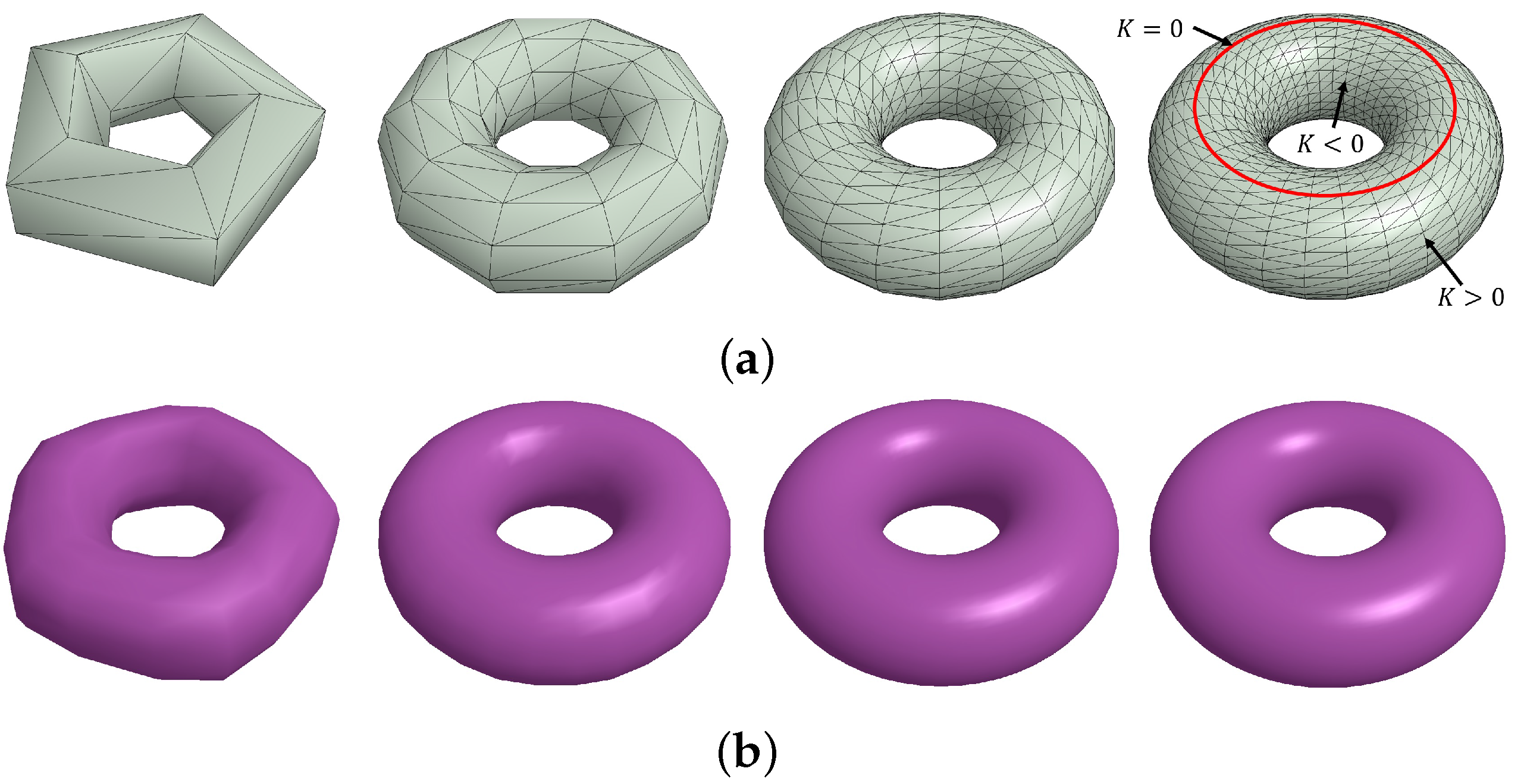
Our last example is a torus which has various distributions of Gaussian curvature as shown in Figure 8a. Table 3 compares two surface areas of polygon meshes and the reconstructed surfaces in Figure 8. The third column lists the surface areas and computation times measured from polygon meshes and the fourth column lists those from the reconstructed surfaces. The next two columns show errors between measured areas and the exact one ( 8 π 2 78 . 9568352 ), and their ratios are shown in the last column.
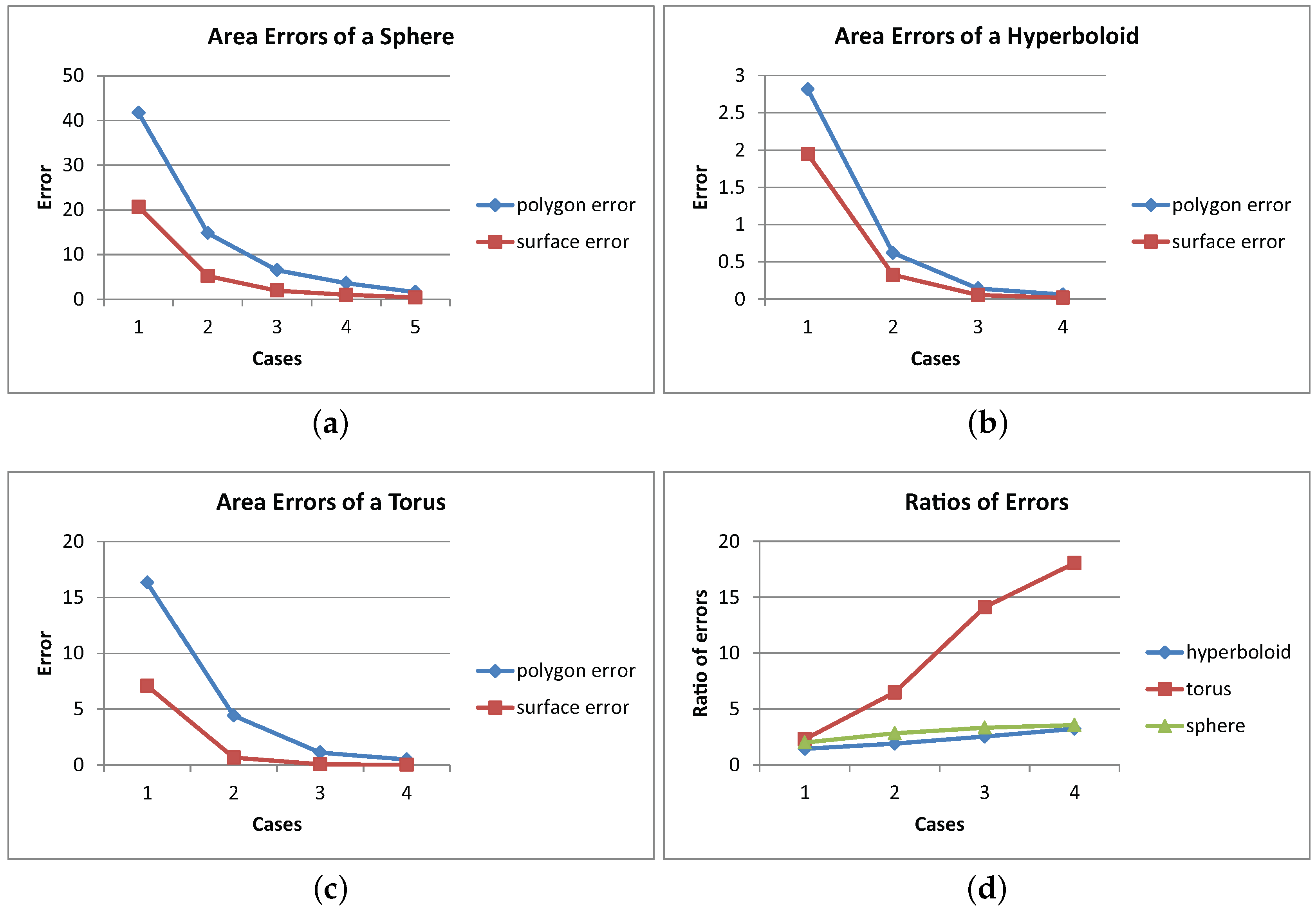
Figure 9 shows graphical illustrations of Table 1, Table 2 and Table 3. Compared with a sphere ( K > 0 ) and a hyperboloid ( K < 0 ), the surface reconstruction of a torus gives much smaller errors as shown in Figure 9d, which means our method gives more accurate results for the objects with various curvature distributions such as human body skin. Therefore, the surface reconstruction can be an effective method for measuring surface areas on 3D scanned human data.

4. Experimental Results

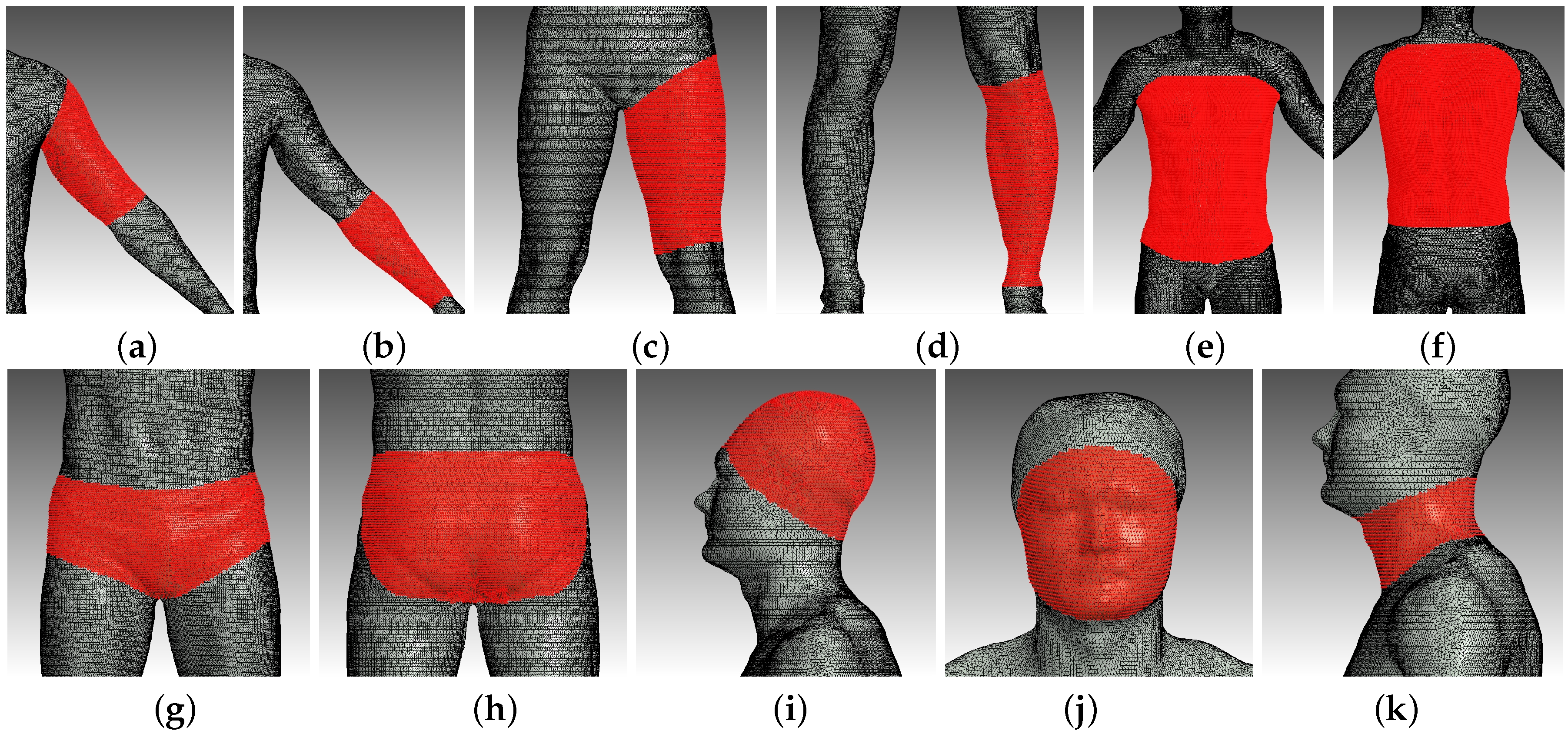
We implemented our technique in C++ (Microsoft Visual C++ 2015) on a PC with an Intel Core i7 2.00 GHz CPU with 8GB of main memory and an Intel ® Iris Pro Graphics 5200. In this section, we explain our experiment results of area computation and compare the results with those obtained by using alginate. We measure areas using alginate and compute areas using the proposed method from 8 subjects. Figure 10 shows a 3D scanned human model with different rendering options. We select 15 regions of interest to measure area: upper arms, lower arms, upper legs, lower legs, abdomen, back, pelvis, hips, head, face, and neck. Figure 11 shows examples of the selected regions of interest.
We use the ratio of the difference to the average value to evaluate similarity as follows:
s i m i l a r i t y = 1 A d f A a v ,
where A a g is the area value measured by using alginate, A s f is the area value computed by surface reconstruction, and A a v is the average value of A a g and A s f . A d f is the difference from the average and A d f = | A s f A a v | = | A a g A a v | . We get the final similarity value for each body part by averaging eight similarity values of eight pairs of area values for each body part.
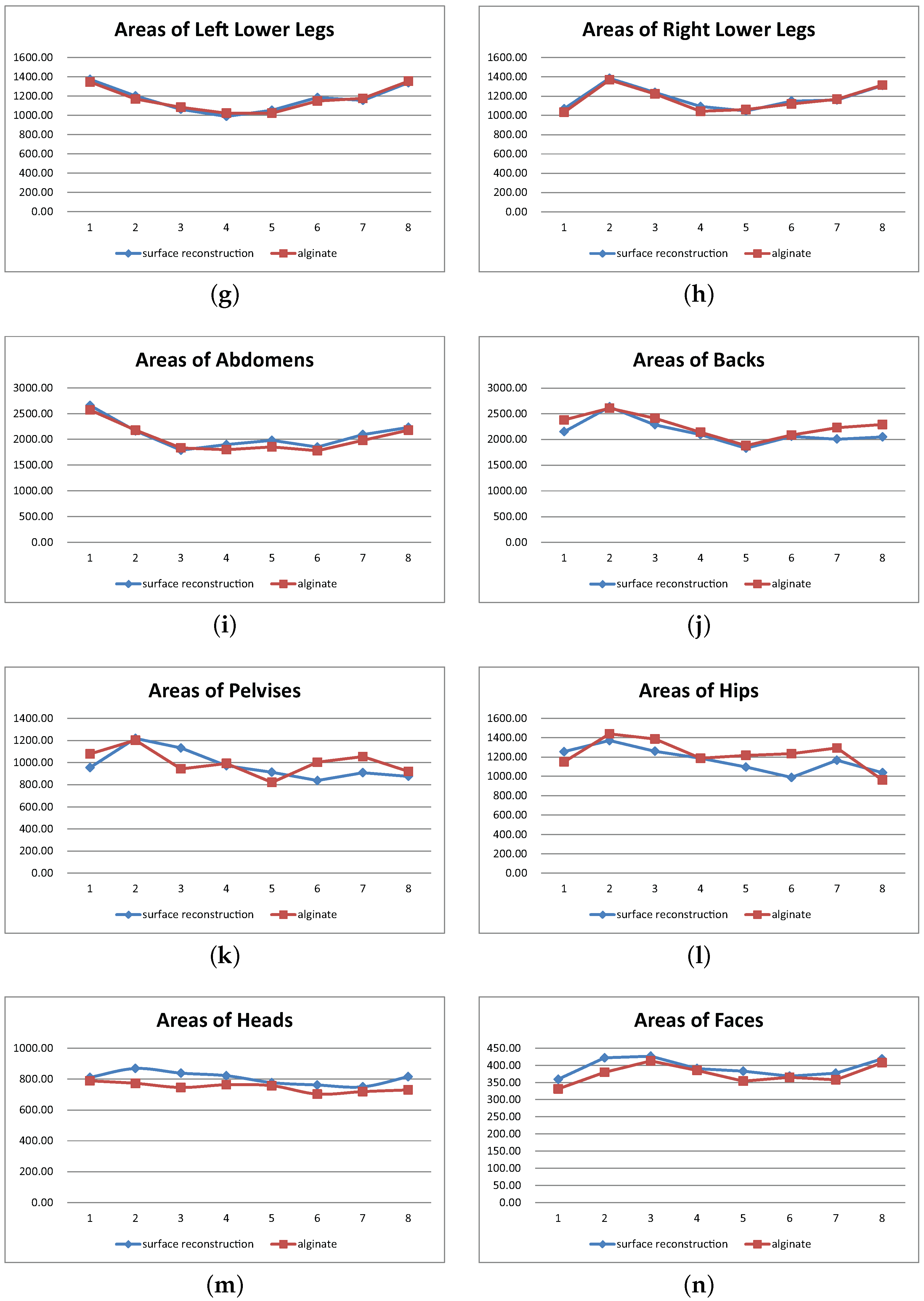
Figure 12 shows eight pairs of area values of various body parts, which are used in the similarity computation. The similarity values of upper arms, lower arms, upper legs, and lower legs are very high, ranging from 97% to 99% (see Figure 12a–h). The correlations between two area values in those body parts are >0.82. The similarity values in the pelvis and hips are slightly low, being about 95%. Sharp foldings in these parts bring in error in area measurement. Table 4 lists all similarity and correlation values of local body parts.
Finally, we should recall that both area values from alginate and from the proposed surface reconstruction method are not true values. As mentioned before, error is inevitably included in the process of projecting 3D surface onto a 2D plane and it is also attributable to human operators who model surfaces and measure surface area by using alginate. In using surface reconstruction, selected regions are different for different operators. Error is expected to be reduced when expert operators measure the areas with both methods repeatedly. We concentrate on the similarity and correlation between the two results in this work.
We have also measured the computation time of our method that includes surface reconstruction and area computation. Compared to the simplest polygon area computation method, our method takes more time as reported in Section 3. However, the absolute time is sufficiently short to be called real-time. In our work, a 3D scanned human model has 250,000 triangles averagely, a face part with 3000 triangles and a back with 25,000 triangles took 24 ms and 206 ms to compute their surface areas, respectively.

5. Conclusions

In this paper, we developed an analytic area computation method by reconstructing a smooth surface from polygonal meshes. We applied this method to measure the areas of local body parts of 3D scanned human models. We also measured areas of the same body parts using the traditional alginate method to compare area computation results. The results showed 95% similarity between the two methods, and we expect our area computation method can be an efficient alternative to using alginate.
In future work, we plan to extend our technique to measure the volume of volumetric data obtained from computed tomography or magnetic resonance imaging, which can be expected to be a useful diagnostic technique in the medical industry.

Acknowledgments

This research was supported by the Basic Science Research Program through the National Research Foundation of Korea(NRF) funded by Ministry of Education(Grant No. NRF-2013R1A1A4A01011627) and also supported by Broadcasting and Telecommunications Development Fund through the Korea Radio Promotion Association(RAPA) funded by the Ministry of Science, ICT & Future Planning.

Author Contributions

Seung-Hyun Yoon and Jieun Lee conceived and designed the experiments; Jieun Lee performed the experiments; Jieun Lee analyzed the data; Seung-Hyun Yoon contributed analysis tools; Seung-Hyun Yoon and Jieun Lee wrote the paper.

Conflicts of Interest

The authors declare no conflicts of interest.

References

  1. Lee, K.Y.; Mooney, D.J. Alginate: Properties and biomedical applications. Prog. Polym. Sci. 2012, 37, 106–126. [Google Scholar] [CrossRef] [PubMed]
  2. 3D Geomagic. Available online: http://www.geomagic.com/en/products/capture/overview (accessed on 16 March 2016).
  3. Whole Body 3D Scanner (WBX). Available online: http://cyberware.com/products/scanners/wbx.html (accessed on 16 March 2016).
  4. LaserDesign. Available online: http://www.laserdesign.com/products/category/3d-scanners/ (accessed on 16 March 2016).
  5. TRIOS. Available online: http://www.3shape.com/ (accessed on 16 March 2016).
  6. Exocad. Available online: http://exocad.com/ (accessed on 16 March 2016).
  7. Tikuisis, P.; Meunier, P.; Jubenville, C. Human body surface area: Measurement and prediction using three dimensional body scans. Eur. J. Appl. Physiol. 2001, 85, 264–271. [Google Scholar] [CrossRef] [PubMed]
  8. Yu, C.Y.; Lo, Y.H.; Chiou, W.K. The 3D scanner for measuring body surface area: A simplified calculation in the Chinese adult. Appl. Ergon. 2003, 34, 273–278. [Google Scholar] [CrossRef]
  9. Yu, C.Y.; Lin, C.H.; Yang, Y.H. Human body surface area database and estimation formula. Burns 2010, 36, 616–629. [Google Scholar] [CrossRef] [PubMed]
  10. Lee, J.Y.; Choi, J.W. Comparison between alginate method and 3D whole body scanning in measuring body surface area. J. Korean Soc. Cloth. Text. 2005, 29, 1507–1519. [Google Scholar]
  11. Vlachos, A.; Peters, J.; Boyd, C.; Mitchell, J.L. Curved PN Triangles. In Proceedings of the 2001 Symposium on Interactive 3D Graphics (I3D ’01), Research Triangle Park, NC, USA, 19–21 March 2001; ACM: New York, NY, USA, 2001; pp. 159–166. [Google Scholar]
  12. Vida, J.; Martin, R.; Varady, T. A survey of blending methods that use parametric surfaces. Computer-Aided Des. 1994, 26, 341–365. [Google Scholar] [CrossRef]
  13. Choi, B.; Ju, S. Constant-radius blending in surface modeling. Computer-Aided Des. 1989, 21, 213–220. [Google Scholar] [CrossRef]
  14. Lukács, G. Differential geometry of G1 variable radius rolling ball blend surfaces. Computer-Aided Geom. Des. 1998, 15, 585–613. [Google Scholar] [CrossRef]
  15. Hartmann, E. Parametric Gn blending of curves and surfaces. Vis. Comput. 2001, 17, 1–13. [Google Scholar] [CrossRef]
  16. Song, Q.; Wang, J. Generating Gn parametric blending surfaces based on partial reparameterization of base surfaces. Computer-Aided Des. 2007, 39, 953–963. [Google Scholar] [CrossRef]
  17. Grimm, C.M.; Hughes, J.F. Modeling Surfaces of Arbitrary Topology Using Manifolds. In Proceedings of the 22nd Annual Conference on Computer Graphics and Interactive Techniques (Siggraph ’95), Los Angeles, CA, USA, 6–11 August 1995; ACM: New York, NY, USA, 1995; pp. 359–368. [Google Scholar]
  18. Cotrina-Navau, J.; Pla-Garcia, N. Modeling surfaces from meshes of arbitrary topology. Computer-Aided Geom. Des. 2000, 17, 643–671. [Google Scholar] [CrossRef]
  19. Cotrina-Navau, J.; Pla-Garcia, N.; Vigo-Anglada, M. A Generic Approach to Free Form Surface Generation. In Proceedings of the Seventh ACM Symposium on Solid Modeling and Applications (SMA ’02), Saarbrucken, Germany, 17–21 June 2002; ACM: New York, NY, USA, 2002; pp. 35–44. [Google Scholar]
  20. Ying, L.; Zorin, D. A simple manifold-based construction of surfaces of arbitrary smoothness. ACM Trans. Graph. 2004, 23, 271–275. [Google Scholar] [CrossRef]
  21. Yoon, S.H. A Surface Displaced from a Manifold. In Proceedings of Geometric Modeling and Processing (GMP 2006), Pittsburgh, PA, USA, 26–28 July 2006; Springer: New York, NY, USA, 2006; pp. 677–686. [Google Scholar]
  22. Vecchia, G.D.; Jüttler, B.; Kim, M.S. A construction of rational manifold surfaces of arbitrary topology and smoothness from triangular meshes. Computer-Aided Geom. Des. 2008, 29, 801–815. [Google Scholar] [CrossRef]
  23. Vecchia, G.D.; Jüttler, B. Piecewise Rational Manifold Surfaces with Sharp Features. In Proceedings of the 13th IMA International Conference on Mathematics of Surfaces XIII, York, UK, 7–9 September 2009; pp. 90–105.
  24. Tomas, A.; Eric, H. Real-Time Rendering; AK Peters: Natick, MA, USA, 2002. [Google Scholar]
  25. Farin, G. Curves and Surfaces for CAGD: A Practical Guide, 5th ed.; Morgan Kaufmann: Burlington, MA, USA, 2002. [Google Scholar]
Figure 1. Measuring the surface area of a hand by using alginate [1].
Symmetry 08 00067 g001
Figure 2. Selected region (in red) from the user’s 2D sketch (in blue).
Symmetry 08 00067 g002
Figure 3. Charts U i and U j and their transition function θ i j ( z ) .
Symmetry 08 00067 g003
Figure 4. (a) Chart U i ; (b) P i ( u , v ) of v i defined on U i .
Symmetry 08 00067 g004
Figure 5. Construction of a blending function.
Symmetry 08 00067 g005
Figure 6. (a) Polygon approximations to a sphere of radius = 5 cm; (b) blending surfaces reconstructed from (a).
Symmetry 08 00067 g006
Figure 7. (a) Polygon approximations to a hyperboloid x 2 + y 2 z 2 = 1 ; (b) blending surfaces reconstructed from (a).
Symmetry 08 00067 g007
Figure 8. (a) Polygon approximations to a torus of radii r = 1 cm and R = 2 cm; (b) smooth blending surfaces reconstructed from (a).
Symmetry 08 00067 g008
Figure 9. Comparison of errors of (a) a sphere; (b) a hyperboloid and (c) a torus; (d) ratios of polygon error to surface error.
Symmetry 08 00067 g009
Figure 10. A 3D scanned human model with different rendering options: (a) skin texture; (b) front view; (c) back view; (d) side view; (e) wireframe.
Symmetry 08 00067 g010
Figure 11. Selected regions of interest: (a) left upper arm; (b) left lower arm; (c) left upper leg; (d) left lower leg; (e) abdomen; (f) back; (g) pelvis; (h) hips; (i) head; (j) face; (k) neck.
Symmetry 08 00067 g011
Figure 12. Areas of body parts of eight people. The red broken line shows eight values of area obtained by using alginate and the blue line shows those obtained by surface reconstruction; (a) areas of left upper arms; (b) areas of right upper arms; (c) areas of left lower arms; (d) areas of right lower arms; (e) areas of left upper legs; (f) areas of right upper legs; (g) areas of left lower legs; (h) areas of right lower legs; (i) areas of abdomens; (j) areas of backs; (k) areas of pelvises; (l) areas of hips; (m) areas of heads; (n) areas of faces; (o) areas of necks.
Symmetry 08 00067 g012aSymmetry 08 00067 g012bSymmetry 08 00067 g012c
Table 1. Comparison of surface areas (in cm 2 ) and computation time (in ms) in Figure 6.
Cases# of TrianglesArea (time) (a)Area (time) (b)Error (1)Error (2)(1)/(2)
160272.46179 (0.03)293.46164 (3)41.6974720.697632.01460
2180299.35513 (0.05)308.94577 (9)14.804135.213492.83958
3420307.64926 (0.06)312.20694 (22)6.5100041.952333.33449
4760310.52105 (0.11)313.14139 (40)3.6382081.017883.57431
51740312.55352 (0.18)313.73544 (92)1.6057380.423823.78871
Table 2. Comparison of surface areas (in cm 2 ) and computation time (in ms) in Figure 7.
Cases# of TrianglesArea (time) (a)Area (time) (b)Error (1)Error (2)(1)/(2)
13217.19809 (0.03)18.06601 (2)2.817231.949311.44524
216219.39459 (0.05)19.68971 (8)0.620730.325611.90636
372219.87309 (0.09)19.95923 (37)0.142230.056092.53575
4168219.95392 (0.17)19.99632 (89)0.06140.0193.23158
Table 3. Comparison of surface areas (in cm 2 ) and computation time (in ms) in Figure 8.
Cases# of TrianglesArea (time) (a)Area (time) (b)Error (1)Error (2)(1)/(2)
15062.64104 (0.04)71.86401 (3)16.315807.092832.30032
220074.53550 (0.05)78.27505 (12)4.421340.681796.48495
380077.82805 (0.1)78.87682 (45)1.128790.0800214.10562
4180078.45343 (0.18)78.92898 (98)0.503410.0278618.06795
Table 4. Similarity and correlation between the results of alginate and the proposed surface reconstruction methods.
RegionSimilarityCorrelation
left upper arm0.992329200.98651408
right upper arm0.990504250.97836923
left lower arm0.974424920.94239832
right lower arm0.975655530.88847152
left upper leg0.969048810.82351873
right upper leg0.972946870.91311208
left lower leg0.988096280.97643038
right lower leg0.990319740.98423465
abdomen0.981089570.97599424
back0.972193780.89756368
pelvis0.948440350.50870081
hips0.953678370.64129904
head0.962747360.63287971
neck0.973414370.88813431
face0.975053720.87872788
average0.949251000.75430084