Article

Unmanned Aerial Vehicle Flight Point Classification Algorithm Based on Symmetric Big Data

1
Department of Computer Engineering, Keimyung University, Daegu 42601, Korea
2
Department of Computer Science and Engineering, Seoul National University of Science and Technology, Seoul 01811, Korea
3
Faculty of Computer Engineering, Keimyung University, Daegu 42601, Korea
*
Author to whom correspondence should be addressed.
Symmetry 2017, 9(1), 1; https://doi.org/10.3390/sym9010001
Submission received: 27 September 2016 / Revised: 8 December 2016 / Accepted: 14 December 2016 / Published: 24 December 2016
(This article belongs to the Special Issue Scientific Programming in Practical Symmetric Big Data)

Abstract

:
Unmanned aerial vehicles (UAVs) with auto-pilot capabilities are often used for surveillance and patrol. Pilots set the flight points on a map in order to navigate to the imaging point where surveillance or patrolling is required. However, there is the limit denoting the information such as absolute altitudes and angles. Therefore, it is required to set the information accurately. This paper hereby proposes a method to construct environmental symmetric big data using an unmanned aerial vehicle (UAV) during flight by designating the imaging and non-imaging points for surveillance and patrols. The K-Means-based algorithm proposed in this paper is then employed to divide the imaging points, which is set by the pilot, into K clusters, and K imaging points are determined using these clusters. Flight data are then used to set the points to which the UAV will fly. In our experiment, flight records were gathered through an UAV in order to monitor a stadium and the imaging and non-imaging points were set using the proposed method and compared with the points determined by a traditional K-Means algorithm. Through the proposed method, the cluster centroids and cumulative distance of its members were reduced by 87.57% more than with the traditional K-Means algorithm. With the traditional K-Means algorithm, imaging points were not created in the five points desired by the pilot, and two incorrect points were obtained. However, with the proposed method, two incorrect imaging points were obtained. Due to these two incorrect imaging points, the two points desired by the pilot were not generated.

1. Introduction

Recently, Unmanned Aerial Vehicles (UAVs) [1] have been flown autonomously to record images for surveillance and patrols. UAVs are becoming increasingly useful for surveillance and patrols because their cost of UAVs is decreasing and the cameras equipped in UAVs also provide cost-effective resolution that is sufficient resolution for surveillance and patrolling tasks at a low price. In order to monitor and fly around a target zone, there have been several studies on flying UAVs autonomously using global positioning system (GPS) [2]. The UAV creates a path that circles a target to obtain images of it, and the UAV and camera are controlled based on this created path. There are also studies that create a short flight path to enable a UAV to obtain images of various targets mid-flight [3,4,5]. The image targets are specified and the UAV seeks the shortest path that will enable it to obtain images of these various targets. Another study proposed the motor primitive structure needed in order to set a surveillance point [6]. There is also a study that adjusts the execution time for the motor primitives so that they are identical at each surveillance point. The motor primitive is set to fly to the surveillance point using the movement of a UAV.
In order to fly UAVs autonomously, a method to set the flight path is required. The user can directly create the UAV’s flight path based on GPS [7,8], but a method to derive and specify a flight path automatically is in high demand. For example, Park [9] specifies a flight path for an auto-pilot flight with affordable control costs by avoiding various obstacles on the surface that could threaten the flight. A waypoint is usually sought based on a contour line, and a flight path that passes the waypoint is determined using Dijkstra’s algorithm. The path with the most affordable cost is then selected for the actual flight. However, because the flight path has been equally partitioned during the grouping process, it is difficult to use such a method if the initial flight points are unbalanced. In order to specify the point to which the UAV will fly, there is the disadvantage that information about the contour lines that the UAV will fly along is required. However, there are additional equipment and costs involved in building data about these contour lines. A method for designating the point for obtaining images is also required. It is possible to designate the UAV’s flight point using three-dimensional (3D) environmental data [10,11,12]. A 3D map needs to be created for the environment through which the UAV will fly, and the target point of the UAV is set using this map. A flight path in which the UAV will not crash can also be created. However, a 3D map must be created in order to determine the flight point. A method is required in which a pilot can quickly create a path without a 3D map.
In order to set a flight path for UAV surveillance and patrols, the following three requirements are necessary. First, there must be a method for automatically setting the flight path. If a pilot directly sets the flight path based on GPS, its accuracy is limited. Moreover, a method that displays the flight path on a map makes it more difficult to set the absolute altitude. By setting the flight path automatically, a more detailed flight path can be determined in 3D space. Second, it must be easy and inexpensive to collect the information required to automatically set the flight path. If the cost or time needed to collect the required information increases, the cost and time needed to automatically create the flight path increase accordingly. For example, obtaining 3D topographical data for flight paths incurs high production costs. Third, the data analysis required for creating a flight path must be automatic. In order to set the flight path automatically, both the data analysis and subsequent flight path creation need to be performed automatically.
This paper proposes a method that automatically categorizes a flight point based on the points that were and were not recorded by a pilot while flying a UAV for surveillance. The flight path is prepared by collecting the records of UAV flights performed by the pilot. The collected data are analyzed using the K-Means algorithm [13] to deduce the optimal points for obtaining images. The points that set the flight path are created using environment data from piloted UAV flight collected in advance. If a UAV can be controlled, the point to which the UAV will fly can also be set. However, if there are errors involved during the data collection process, the point for obtaining images will be changed as a result of these errors. No additional equipment is required to create the environmental data needed for surveillance in advance. It is hence possible to easily create the flight path based on the points for obtaining images and monitoring.
This paper is organized as follows: Section 2 reviews related work. Section 3 introduces the definitions that are necessary to categorize the flight points that were collected through the UAV and proposes a method that categorizes the points for obtaining images as well as the non-imaging. Section 4 validates the proposed method by collecting pilot data and generating a flight path. Section 5 discusses and verifies the proposed method by categorizing the pilot-collected imaging points and non-imaging points that were collected by a pilot. Finally, Section 6 concludes this paper.

2. Related Work

There is a method for creating flight paths to enable multiple UAVs to monitor a moving target [2,14]. This method creates a circulating path that the UAVs travel in order to obtain images while flying alongside a moving target. The UAVs fly autonomously along the created path and the target is recorded. However, there is the possibility that a UAV could crash into obstacles on the surface or in urban areas while circling around the target. A method is required to designate the points through which the UAV can travel above the surface or in urban areas.
There are also genetic algorithm-based methods for creating a low cost flight path in order to monitor targets in the center of a city while taking images of the city from the sky [3,4]. More targets can be observed at a low cost by controlling the height of the UAV in the air. However, because of the fixed angle of the UAV cameras, targets cannot be recorded in some cases because they are occluded by buildings. In [5], the gimbal of the camera is controlled in order to take more images of occluded targets during flight along a path. As a result, the targets can be recorded at a low cost by reducing the number of target imaging points hidden by buildings. However, while the UAV can record multiple targets from the sky, it is difficult to take images of targets that are attached to the sides of buildings or the target.
There is a study on correcting the GPS so that a UAV may fly autonomously based on waypoints in the external environment [7,8]. A Kalman filter is used to make corrections by combining the IMU (Inertia Measurement Unit) sensor on the UAV and GPS so that the pilot can fly the UAV according to the designated waypoint. It has a simple UI (User Interface) structure that the pilot can use to set the GPS waypoints for the path that the UAV will fly autonomously. However, it is difficult to provide a UI that can set the image angle, absolute altitude, and other parameters of the imaging point as the UAV flies along the path. In order for the pilot to set the UI, information is required that must be given to the pilot in advance.
There is a study on creating a flight path based on environmental data such as the point of obstacles [10,11,12]. Environmental data for the UAV’s flight are built in advance, and the UAV’s flight path is generated according to these environmental data. However, additional equipment is required in order to build data on the external environment of the region where the UAV will monitor while flying. A method to designate the point where the UAV must fly without additional equipment is required in many situations.
In [15], the actions of a robot are created by analyzing its movements. Using the records of a human’s control over a robot, this method creates the actions to control the robot. However, because the UAV can be influenced by the external environment during its flight, it is difficult to locate the UAV to the desired destination precisely according to control signals alone.
There is a method that can create the motor primitives needed to fly for identical periods of time across an indoor parking lot using a UAV [6]. Demo-based learning is used to learn the state and control signals needed to fly through an indoor parking lot, and the user can fly the UAV to a desired destination according to these state and control signals. In [16], the motor primitives for flying a UAV to an outside surveillance point are defined. Motor primitives are created using the UAV state data collected by the user and the surveillance point specified by the pilot. This method requires the user’s pilot records to specify the flying point and select the flight path in advance.
In the proposed method, a flight point generating method in which the pilot verifies images shot by the UAV camera is proposed to solve issues such as the UAV’s camera zoom in/out limitations, and the inability of the pilot to determine the imaging direction of the facilities. In order to solve issues caused by a complex UI in which the UAV’s absolute altitude with respect to flight path and the imaging angle of facilities must be set, a method in which the pilot sets them intuitively during the UAV’s flight is explained. Since pilot errors and measurement errors of the UAV’s sensor are included during the process in which the UAV’s autonomous flight path is generated, a method in which the UAV’s autonomous flight points are generated after removing such errors is proposed.

3. Overview of Flying Points

This paper proposes a method for expressing UAV flight points, for analyzing recorded UAV flight points and for generating UAV flight paths needed for autonomous flights. Therefore, the recorded UAV flight points are categorized and grouped based on the K-Means algorithm [13] and then are expressed by a graph for UAV flight paths.

3.1. UAV Point and Angle

It is assumed that the surveillance UAV is equipped with one omnidirectional camera. The followings must be considered in order to generate an UAV flight path. First, the GPS-based UAV point must be considered. In outdoor environments, the UAV’s point is generally assumed to be based on GPS, and this point is the most important data for generating a flight path. Second, the direction of the camera on the UAV camera must be considered. If the UAV camera angle differs from the corresponding UAV angle, even at the same GPS point, a monitored target will differ. The UAV’s point P i , j and angle R i , j at index i, which is the flight sequence, and index j, which is the sequence of the points and the rotations during the ith flight. Point P i , j is expressed as 3D UAV coordinates, as shown in Equation (1), where xi,j, yi,j, and zi,j are located on the x-, y-, and z-axes that correspond to the GPS longitude, GPS latitude, and absolute altitude, respectively.
P i , j = [ x i , j , y i , j , z i , j ]
Angle R i , j involves the x-axis angle ϕ i , j , y-axis angle θ i , j , and z-axis angle φ i , j and determines the degree of the UAV’s camera angle for each axis, as show in Equation (2).
R i , j = [ ϕ i , j , θ i , j , φ i , j ]

3.2. Expression of the UAV Flight Points

The five types of points that are required to generate paths are defined as follows. Surveillance point is the points where an UAV obtains images during flight. Takeoff point B is the point at which the collection of the UAV’s state begins and is expressed using the x-, y-, and z-coordinates. In other words, the point from which flight records are collected for autonomous flight is called takeoff point B . The UAV departs from the takeoff point and begins its flight. It is assumed that the takeoff point B is limited to one point; nevertheless multiple takeoff points may be designated in principle.
Goal point L is the point where the flight ends after imaging of the surveillance point is complete. This point also includes the x-, y-, and z-coordinates. The UAV lands at the goal point L , and it is assumed that goal point L is also limited to one point in the proposed method.
During the pilot’s flying process, facilities are not imaged in all the points over which the UAV flies. In actuality, facilities can not be imaged in points where they should be. Therefore, flight points are classified into imaging points and points of flight toward imaging points. It is true that the image angle of facilities is important at imaging points, however, in flying points, the imaging angle is not important because facilities are not captured by the camera, which is why it is not considered.
Imaging point W i , q is defined as the point from which the UAV observes the qth imaging point in the ith flight. Imaging point W i , q is defined, as shown in Equation (3), which includes index i, index q, which is the imaging point, and index ji,q, which is which is the measuring sequence of the point P i , j and the angle R i , j , UAV point P i , q , and angle R i , q . Imaging point set W, which is a collection of imaging points, contains all set imaging points.
W i , q = [ i ,   q ,   j i , q ,   P i , q ,   R i , q ]
Non-imaging point U i , j is defined as the flying point of the UAV and includes index i, index j, and the UAV point P i , j , as shown in Equation (4). Non-imaging point set U, which is the collection of non-imaging points, includes takeoff point B , and goal point L ( B U, L U).
U i , j = [ i ,   j ,   P i , j ]
For examples, the two flight paths are determined by takeoff point B , goal point L , imaging point set W, and non-imaging point set U, as shown in Figure 1. In the imaging points, points and angles are set to obtain images of surveillance points as follow. The two imaging points obtaining the images of one surveillance point are set during the first flight and second flight.

3.3. Normalization of Imaging and Non-Imaging Points

During the classification of the imaging and non-imaging points to which the UAV has flown, points and angles are compared even though they have different units. Therefore, all units are converted into relative ratios by normalizing them for comparison. In order to normalize the points and angles, the maximum and minimum of each element of the points and angles are defined as shown in Table 1 and Table 2. Among the points included in the set of non-imaging point set U, the set of all points that represent the x-axis points is defined as P x . The set of all points that represent the y-axis points is defined as P y , and the set of all points that represent the z-axis points is defined as P z . Regarding the imaging point set W, all angles located on the x-axis are defined as the set of angles R ϕ , all angles located on the y-axis are defined as the set of angles R θ , and all angles located in the z-axis are defined as the set of angles R φ .
The maximum and minimum values of all elements included in P x , P y , and P y are restored through functions M A X and M I N . Functions M A X and M I N are used to restore the maximum and minimum values included in all angles for R ϕ , R θ , and R φ .
The normalized imaging point set W’ is a collection of normalized imaging points. The normalized qth normalized imaging point W i , q is defined as shown in Equation (5). The normalizations for each element of point P i , q , and angle R i , q are shown in Equation (6). In this normalization process, if the normalized element is greater than the maximum value, it is set to 1, and it is set to 0 if it is less than the minimum value.
W i , q = [ i ,   q ,   j i , q   P i , q ,   R i , q ]
where P i , q = [ x i , q , y i , q , z i , q ] , R i , q = [ ϕ i , q , θ i , q , φ i , q ] .
x i , q = x i , q M I N ( P x ) M A X ( P x ) M I N ( P x ) ,   y i , q = y i , q M I N ( P y ) M A X ( P y ) M I N ( P y ) ,   z i , q = z i , q M I N ( P z ) M A X ( P z ) M I N ( P z ) ϕ i , q = ϕ i , q M I N ( R ϕ ) M A X ( R ϕ ) M I N ( R ϕ ) ,   θ i , q = θ i , q M I N ( R θ ) M A X ( R θ ) M I N ( R θ ) ,   φ i , q = φ i , q M I N ( R φ ) M A X ( R φ ) M I N ( R φ )
The normalized non-imaging point set U’ is the collection of normalized non-imaging points. The jth normalized non-imaging point U i , j is defined, as shown in Equation (7), using normalized point P i , j . The Normalization for each element of point P i , j categorization is shown in Equation (8).
U i , j = [ i ,   j ,   P i , j ]
where
P i , j = [ x i , j , y i , j , z i , j ] x i , j = x i , j M I N ( P x ) M A X ( P x ) M I N ( P x ) ,   y i , j = y i , j M I N ( P y ) M A X ( P y ) M I N ( P y ) ,   z i , j = z i , j M I N ( P z ) M A X ( P z ) M I N ( P z )

3.4. Weight Establishment

Each element of a point and each element of an angle values have values between 0 and 1 through normalization. However, because the relative weight of each sensor value differs, there must be something that reflects this fact. This paper determines the relative weight by multiplying each weighted value to the normalized value.
The weights for classifying the imaging and non-imaging points are defined as shown in Table 3 and Table 4. Each weight is determined by considering the maximum and minimum values as well as the relative value with consideration of the distribution of the normalized values. For example, the weight ω φ is set by eight considering the directions of a UAV when the directions of the UAV are classified by eight groups.

3.5. Setting Error Range

Each element of a point and each element of an angle on the UAV include a certain error. Errors other than sensor errors are caused by the pilot during the flight. Therefore, these errors must be accounted for in order to categorize the UAV state. Given that the error range differs for each sensor and errors are caused by the pilot during the flight, each range is defined individually. This paper establishes the error tolerances for UAV point and angles categorization in Table 5 and Table 6. Therefore, they are processed as the same value within the error range. The error ranges of each element are normalized using the minimum and maximum values, as shown in Equation (9). Given that the elements of angles are set by 0 as a starting value, the minimum value is not subtracted from each corresponding element.
δ x = δ x M I N ( P x ) M A X ( P x ) M I N ( P x ) ,   δ y = δ y M I N ( P y ) M A X ( P y ) M I N ( P y ) ,   δ z = δ z M I N ( P z ) M A X ( P z ) M I N ( P z ) δ ϕ = δ ϕ M A X ( R ϕ ) M I N ( R ϕ ) ,   δ θ = δ θ M A X ( R θ ) M I N ( R θ ) ,   δ φ = δ φ M A X ( R φ ) M I N ( R φ )

4. K-Means-Based Classification

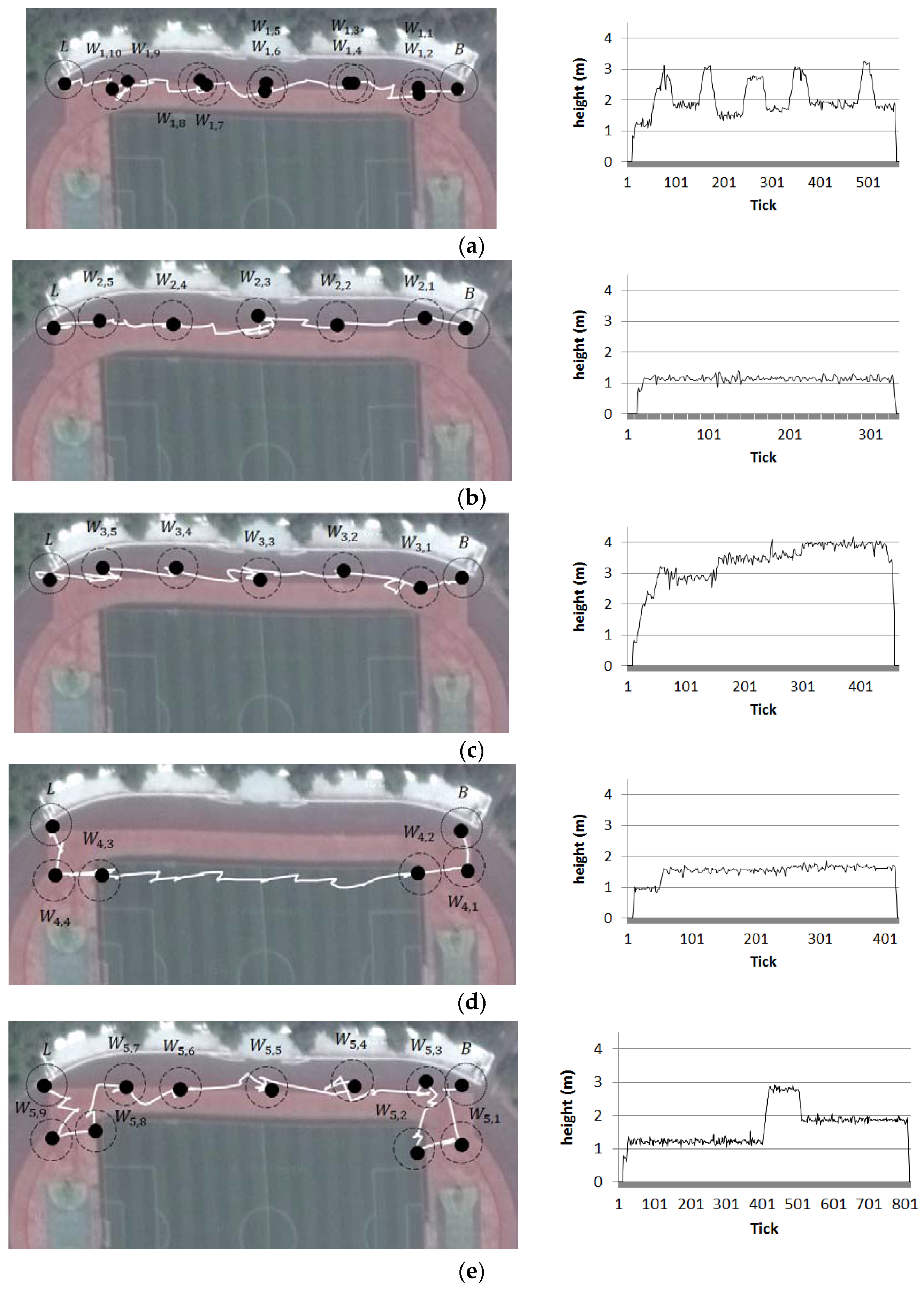
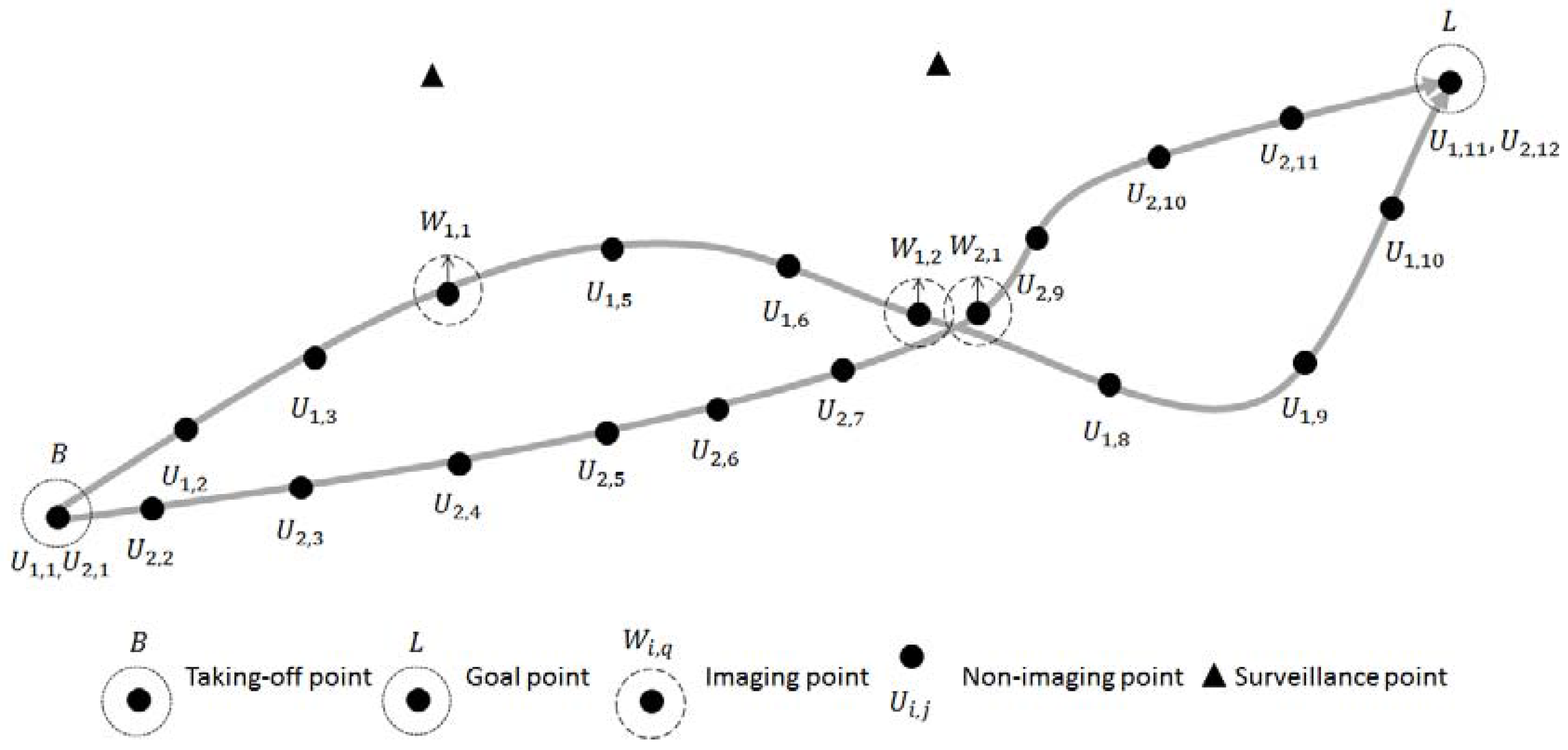
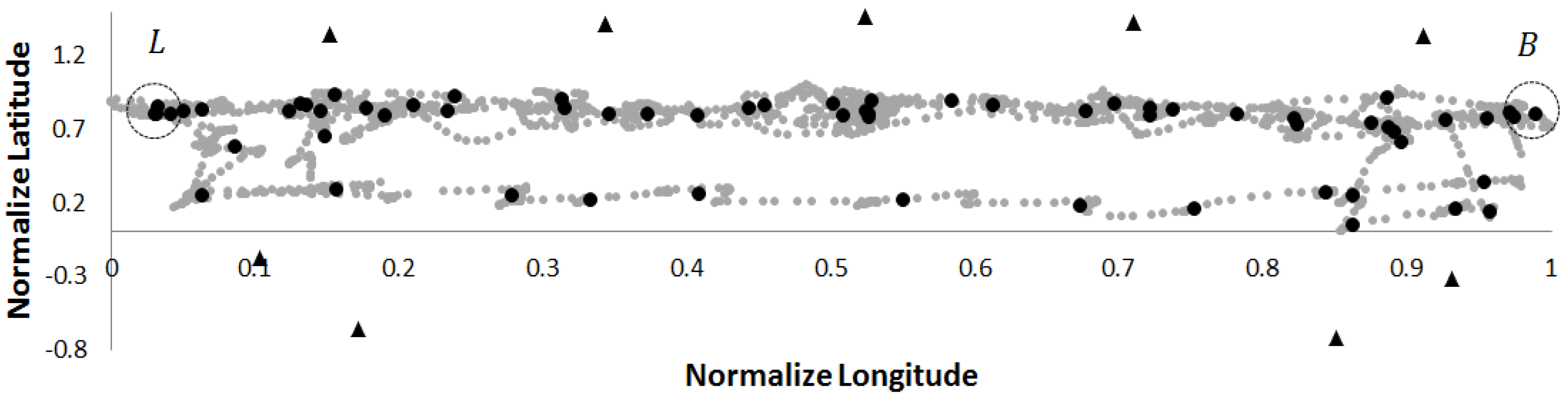
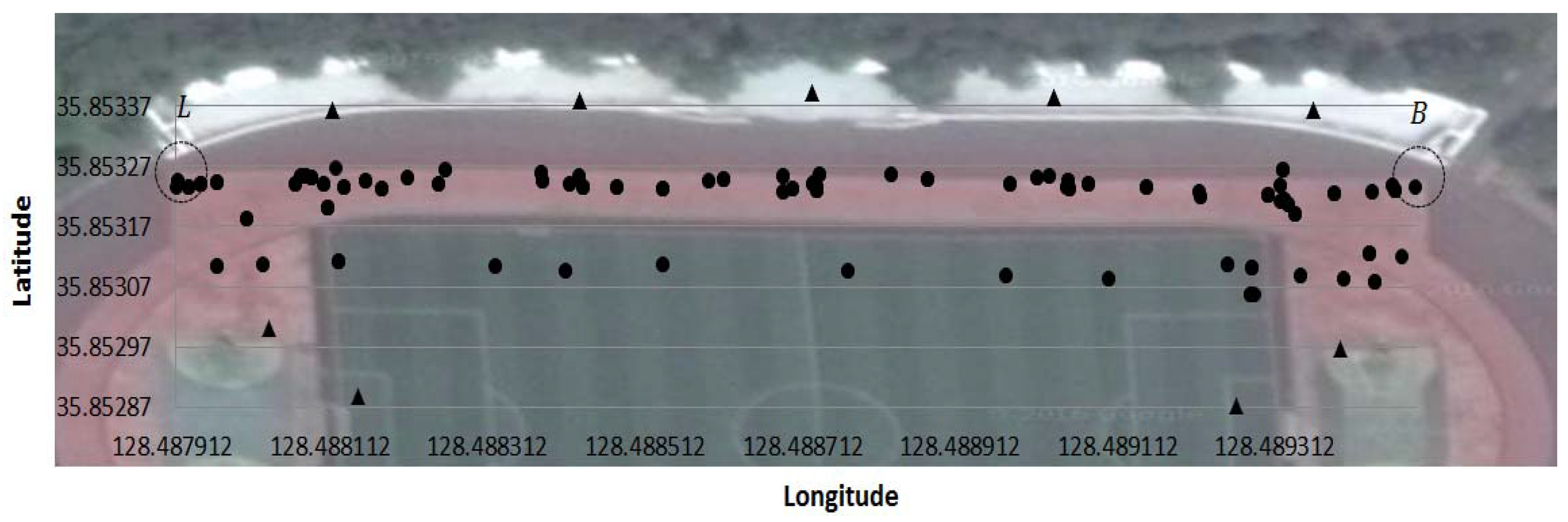
After classifying points as imaging points and non-imaging points of flight toward imaging points, the generation method is introduced. During the process in which the UAV image points surveilled by the pilot, the UAV does not imagine surveillance point at all flight points. Actually, since facilities could not be imaged in points where they should be, flight points are classified into imaging points and points of flight toward imaging points. Although UAV’s imaging angle is important in points where surveillance points are image, it is not important and thus not considered in flight points where surveillance points are not image.

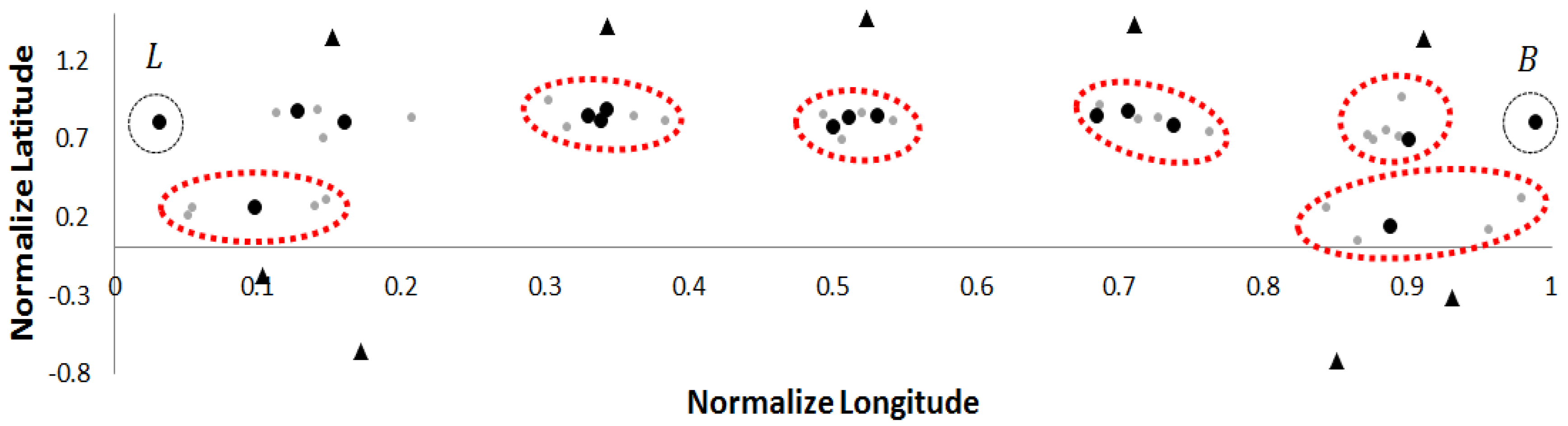
4.1. Definition of Imaging Point and Non-Imaging Point Clusters

In order to determine the flight path on which the UAV will navigate, normalized non-imaging point set U’ is classified and is added to normalized non-imaging point cluster set C’m, which is a collection of normalized non-imaging point clusters defined as shown in Equation (10). The oth normalized non-imaging point cluster, which categorizes a collection of normalized non-imaging points, is defined as normalized non-imaging point cluster C’m,o.
C m = [ C m , 1 , C m , 2 ,   ,   C m , o , ]
Normalized non-imaging point cluster centroid set M m is defined as shown in Equation (11). Normalized non-imaging point cluster C’m,o includes a part of normalized non-imaging point set U’, and the normalized non-imaging point cluster centroid is denoted as μ m , o and defined as [ x m , o , y m , o , z m , o ] .
M m = [ μ m , 1 ,   μ m , 2 ,   ,   μ m , o ,   ]
The finally classified normalized non-imaging point set U’ is defined by the normalized non-imaging point cluster set C’w the normalized non-imaging point cluster centroid set M w .
Set normalized imaging point set W’, which is the collection of normalized imaging points, is also classified identically to normalized non-imaging point cluster set C’m, which is the collection of normalized non-imaging point clusters. Set normalized imaging point cluster set C’n, which is the collection of normalized imaging point clusters during the nth run, is defined as shown in Equation (12). Set normalized imaging point cluster set C’n includes normalized imaging point cluster C’n,g, which is the gth normalized imaging point cluster.
C n = [ C n , 1 , C n , 2 ,   ,   C n , g , ]
Normalized imaging point cluster centroid set M n is defined as shown in Equation (13). Normalized imaging point cluster C’n,g includes some elements of normalized imaging point set W’. The normalized imaging point cluster centroid μ n , g is defined by Equation (14), using normalized point P n , g and angle R n , g .
M n = [ μ n , 1 ,   μ n , 2 ,   ,   μ n , g ,   ]
μ n , g = [ P n , g , R n , g ]
where P n , g = [ x n , g , y n , g , z n , g ] , R n , g = [ ϕ n , g , θ n , g , φ n , g ] .
The finally classified results of the normalized imaging point set W’ are the normalized imaging point cluster set C’v and normalized imaging point cluster centroid set M v .

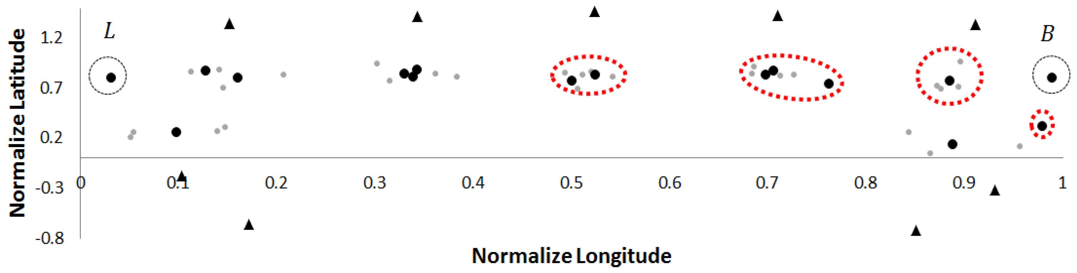
4.2. Normalized Non-Imaging Point Categorization

Categorization of non-imaging points is identical to the conventional K-means algorithm. First, K, the number of the elements of the normalized non-imaging point cluster set C’m, is defined and normalized non-imaging point cluster centroids are set. K is set by considering the total distance in flying during the process of categorizing the non-imaging points. Second, Non-imaging points are classified by utilizing normalized non-imaging point cluster centroid. Third, normalized non-imaging point cluster centroids are adjusted by non-imaging points in re-allocated normalized non-imaging point clusters. Fourth, the second and the third processes are performed repeatedly until there is no change of normalized non-imaging point cluster centroids.
Finally, normalized non-imaging point cluster set C’w and Normalized non-imaging point cluster centroid set M w are created based on non-imaging point set U’.
In the Second step, normalized non-imaging points in normalized non-imaging point set U’ are assigned clusters based on the normalized non-imaging point cluster centroids that were established. In order to categorize normalized non-imaging point U i , j as a normalized non-imaging point cluster member, the similarity is calculated, as shown in Equation (15). Function u ( P i , j , P m , o ) returns the sum of each weighted Euclidean distance of normalized non-imaging point U i , j . Using function u ( P i , j , P m , o ) , the normalized non-imaging point U i , j is added to the normalized non-imaging point cluster with the lowest value, as shown in Equation (16).
u ( P i , j , P m , o ) = ω x × ( x i , j x m , o ) 2 + ω y × ( y i , j y m , o ) 2 + ω z × ( z i , j z m , o ) 2
C m , o = { U i , j : u ( P i , j , P m , o ) u ( P i , j , P m , r ) j , 1 r K }
where each point U i , j is assigned to exactly one normalized non-imaging point cluster C m , o , even if it could be assigned to two or more of them.
In the Fourth step, the stability of the configured non-imaging point cluster centroids is checked. A state of no change is defined the distance between two non-imaging point cluster centroids between pre- and post-alteration of cluster centroids is less than the threshold value ε w , as shown in Equation (17). After checking whether there is a change in the non-imaging point cluster centroids, then the method is ends. If there is a change, the method returns to the Second step.
1 o K u ( P m 1 , o , P m , o ) < ε w  

4.3. Non-Imaging Point Denormalization

The denormalized results of normalized non-imaging point cluster centroid set M w is defined by non-imaging point cluster centroid set M . There are normalized non-imaging point cluster centroids in non-imaging point cluster centroid set M . Normalized non-imaging point cluster centroid is denoted as μ o and defined as [ x o , y o , z o ] . Non-imaging point cluster centroids of non-imaging point cluster centroid set M are created as shown in Equation (18), which has the same number elements with the number of the elements of Non-imaging point cluster centroid set M w .
M = [ μ 1 , μ 2 ,   ,   μ | M w | ]
oth non-imaging point cluster centroid μ o is set by denomalizing each element of the normalized non-imaging point cluster centroid μ w , o as shown in Equation (19).
x o = x w , o × ( M A X ( P x ) M I N ( P x ) ) + M I N ( P x ) , y o = y w , o × ( M A X ( P y ) M I N ( P y ) ) + M I N ( P y ) , z o = z w , o × ( M A X ( P z ) M I N ( P z ) ) + M I N ( P z )

4.4. Normalized Imaging Point Categorization

Non-imaging points do not require accurate positions while surveillance points are designated. However, a method is required to generate imaging points designated by the pilot. In non-imaging points, empty clusters are not generated due to the large quantity of non-imaging points collected, but in imaging points, empty clusters can be generated depending on the amount of imaging points designated by the pilot. During the imaging point categorization process, a method to set cluster center points minimizing the distribution of distance differences is required.
The proposed Bounded K-Means algorithm proceeds as follows. First, K, which is the number of normalized imaging point cluster C’n, is determined, and the normalized imaging point cluster centroids are set. Second, the set normalized imaging point cluster centroids are used to divide normalized imaging points. Third, normalized imaging point cluster centroids are readjusted as normalized imaging points belonging to the reassigned normalized imaging point clusters. Fourth, Steps 2 and 3 are repeated until there is no variation in the normalized imaging point cluster centroids.
During the reassigning process that takes place if the number of imaging points is low and they are widely distributed, empty imaging point clusters can be generated if imaging points exist in the bounding boundary of imaging points. After readjusting normalized imaging point cluster centroids, empty clusters are checked. If an empty normalized imaging point cluster exists and the cost of adding other normalized imaging point cluster members that are out of the error range of their normalized imaging point cluster centroids to this normalized imaging point cluster is less than the current cost, it proceeds to the empty cluster centroid is set to be the normalized imaging point cluster with the lowest cost for all normalized imaging point cluster members that are out of the error range of their own normalized imaging point cluster centroids. The distance between the normalized imaging point cluster centroid and each of its normalized imaging point cluster member is calculated using function d ( P i , q ,   R i , q ,   P n , g ,   R n , g ) as shown in Equation (20). The error range is calculated in err, as shown in Equation (21). Normalized imaging point cluster members that satisfy the out of error range ( d ( P n , g ,   R n , g ,   P i , q ,   R i , q ) e r r > 0 ) from their normalized imaging point cluster centroid are identified. When a normalized imaging point cluster centroid is changed back into a normalized imaging point cluster member, the state with the lowest cost is set as the empty cluster centroid, as shown in Equation (22). The method then proceeds to Step 2.
d ( P i , q ,   R i , q ,   P n , g ,   R n , g ) = ( x i , q x n , g ) 2 + ( y i , q y n , g ) 2 + ( z i , q z n , g ) 2 + ( ϕ i .   q ϕ n , g ) 2 + ( θ i .   q θ n , g ) 2 + ( φ i .   q φ n , g ) 2
e r r   = ( δ x 2 + δ y 2 + δ z 2 + δ ϕ 2 + δ θ 2 + δ φ 2 )
μ n , g = [ P i , q ,   R i , q ]
where i and q are
a r g   min i ,   q ( μ n , g C n W i , q C n , g { i f ( d ( P i , q , R i , q , P n , g , R n , g ) e r r > 0 )    d ( P n , g , R n , g , P i , q , R i , q ) 3   e l s e    0 ) .
It is checked whether two random normalized imaging point cluster centroids are within error range ( d ( P n , g 1 ,   R n , g 1 ,   P n , g 2 ,   R n , g 2 ) e r r   0 ) ) and whether random members are out of the error range of the normalized imaging point cluster centroid using d ( P n , g ,   R n , g ,   P i , q ,   R i , q ) e r r > 0 ) . The normalized imaging point cluster centroid and random normalized imaging point cluster members that satisfy both conditions are used. If changing random members within the error range to the relevant normalized imaging point cluster centroid is lower than the current cost, the method proceeds to when combined as shown in Equation (23), Equation (24) members that are out of the error range are set as centroid points among two of the g1th and g2th imaging point cluster centroids that are within the error range with the lowest cost, the gth normalized imaging point cluster centroid, and the normalized imaging point cluster members. After creating new clusters, the method returns to Step 3. If all two conditions are not met, it proceeds to Step 2.
μ n , g 1 = [ P n , g 1 ,   R n , g 1 ]
where
P n , g 1   i s   1 | C n , g 1 | W i , q C n , g 1 P i , q + 1 | C n , g 2 | W i , q C n , g 2 P i , q , R n , g 1   i s   1 | C n , g 1 | W i , q C n , g 1 R i , q + 1 | C n , g 2 | W i , q C n , g 2 R i , q . μ n , g 2 = [ P i , q ,   R i , q ]
where i and q are
a r g   m i n   i ,   q ( μ n , g C n W i , q C n , g { i f ( d ( P i , q , R i , q , P n , g , R n , g ) e r r > 0 )    d ( P i , q , R i , q , P n , g , R n , g ) 3 e l s e    0 ) .
In Step 2, the members of normalized imaging point set W’ are clustered. In order to cluster normalized imaging point, a similarity is calculated, as shown in Equation (25). Function f ( P i , q ,   R i , q ,   P n , g ,   R n , g ) returns the sum of each weighted Euclidean distance of normalized state. Normalized imaging points are added to the cluster with the lowest such value, as shown in Equation (26).
f ( P i , q ,   R i , q ,   P n , g ,   R n , g ) = u ( P i , q , P n , g ) 2 + ω ϕ × ( ϕ i .   q ϕ n , g ) 2 + ω θ × ( θ i .   q θ n , g ) 2 + ω φ × ( φ i .   q φ n , g ) 2
C n , g = { W i , q : f ( P i , q ,   R i , q ,   P n , g ,   R n , g ) f ( P i , q ,   R i , q ,   P n , r ,   R n , r ) j , 1 r K }
where each normalized imaging point W i , q is assigned to exactly one normalized imaging point cluster C n , g , even if it could be assigned to two or more of them.
In Step 4, the stability of the current cluster centroids is checked. If the distance between two cluster centroids pre- and post-alteration is less than a threshold value ε v , as shown in Equation (27), it is defined as a state of no change for that normalized imaging point cluster. If there is no change in any imaging point cluster, then the method is end. If there is a change, the method returns to Step 2.
1 g K f ( P n 1 , g ,   R n 1 , g ,   P n , g ,   R n , g ) < ε v
Instead of Equations (22) and (24), Equations (28) and (29) can be applied by applying the weight.
μ n , g = [ P i , q ,   R i , q ]
where i and q are
a r g   m i n   i ,   q ( μ n , g C n W i , q C n , g { i f ( d ( P i , q , R i , q , P n , g , R n , g ) e r r > 0 )    f ( P n , g , R n , g , P i , q , R i , q ) 3 e l s e    0 ) .
μ n , g 2 = [ P i , q ,   R i , q ]
where i and q are
a r g   m i n   i ,   q ( μ n , g C n W i , q C n , g { i f ( d ( P i , q , R i , q , P n , g , R n , g ) e r r > 0 )    f ( P i , q , R i , q , P n , g , R n , g ) 3 e l s e    0 ) .

4.5. Normalized Imaging Point Denormalization

This is a method of generation of imaging points that will be actually used which denormalizes the normalized imaging point cluster centroid set M v not to a value of 0 or 1, but to a location and angle values that are actually used. The imaging point cluster centroid set M , which records the denormalized value of the normalized imaging point cluster centroid set M v , is generated. The imaging point cluster centroids of the imaging point cluster centroid set M is generated as shown in Equation (30) as large as the size of the normalized imaging point cluster centroid set M v . The imaging point cluster centroid is denoted as μ g and defined as [ P g ,   R g ] . Here, P g = [ x g , y g , z g ] , R g = [ ϕ g , θ g , φ g ] .
M = [ μ 1 , μ 2 ,   ,   μ | M v | ]
gth imaging point cluster centroid μ g is set by denormalizing the elements of the normalized imaging point cluster centroid μ v , g as show in Equation (31).
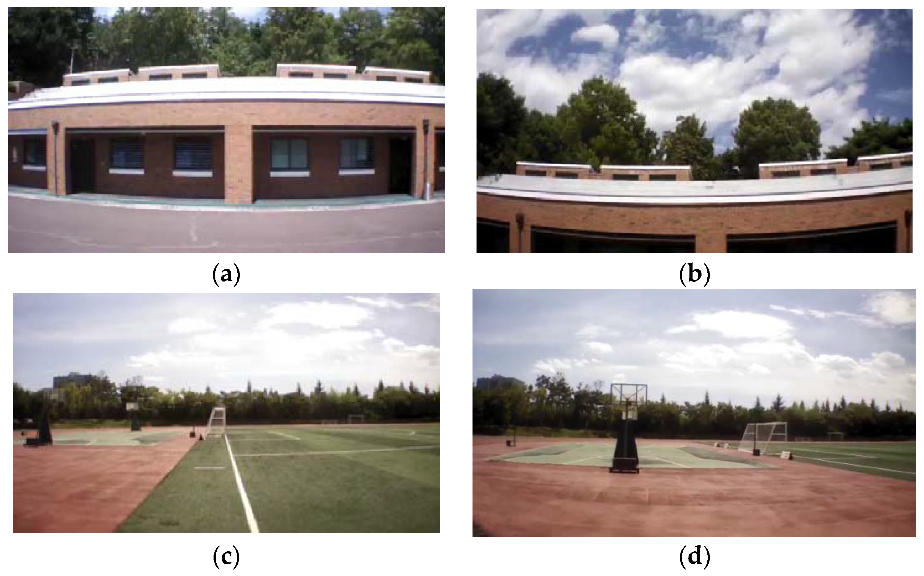
x g = x v , g × ( M A X ( P x ) M I N ( P x ) ) + M I N ( P x ) ,   y g = y v , g × ( M A X ( P x ) M I N ( P y ) ) + M I N ( P y ) ,   z g = z v , g × ( M A X ( P x ) M I N ( P z ) ) + M I N ( P z ) , ϕ g = ϕ v , g × ( M A X ( R ϕ ) M I N ( R ϕ ) ) + M I N ( R ϕ ) ,   θ g = θ v , g × ( M A X ( R θ ) M I N ( R θ ) ) + M I N ( R θ ) ,   φ g = φ v , g × ( M A X ( R φ ) M I N ( R φ ) ) + M I N ( R φ )

5. Experiments

In this section, the environment in which the pilot used the UAV to collect surveillance data. The non-imaging points and imaging points that were collected when the pilot flew the UAV are described, and we define the constants for categorizing imaging and non-imaging points. Finally, we compare the results of imaging points categorized using the proposed method with those categorized using the conventional K-Means algorithm.

5.1. Environment for Flight Path Collection

The points defined for monitoring vandalism and theft at Keimyung University Stadium are shown in Figure 2. The GPS and absolute altitude were set as shown in Table 7. Points for monitoring that overlap on the map show different absolute altitudes. For example, at the points with two overlapping surveillance areas, the club room entrance on the first floor is observed while flying at a first-floor absolute altitude. However, when flying at a second-story absolute altitude, the UAV checks for vandalism in the bleachers on the second floor. Example images of points that the pilot should monitor are shown in Figure 3.

5.2. Collected Flight Path

An AR.Drone 2.0 [17,18] was flown by a pilot to obtain images of the surveillance points and set the flight points. The UAV was flown over 14 different surveillance points to capture images over five different flights. The five collected flight paths with the same takeoff point and goal point are shown in Figure 4. The flight points were collected by flying along different paths and capturing the images from different surveillance points. The paths in Figure 4(a)–(c) appear as the same path. However, they have different absolute altitudes. Thus, the points from which the UAVs obtained the images also differ.

5.3. Definitions of Constant Values

The pilot set the minimum and maximum values shown in Table 8 and Table 9 for the flight region. The x-, y-, and z-axes corresponding to the minimum and maximum values of the points were verified using the non-imaging point set U.
The pilot set the weighted values as shown in Table 10 in order to categorize the imaging points and non-imaging points. The range of the x-axis of flight data was 170 m, that of the y-axis was 15 m, and that of the z-axis was 4. Since the pilot determined the error of the x-axis and y-axis to be approximately 10 m, the weighted value of the x-axis and y-axis were set as 17 and 1.5, respectively. The z-axis flies approximately 4 m with an error of approximately 2 m. Thus, the weighted value of the z-axis was set as 2. Since while the imaging points are obtained when the flight takes place in hovering state, the x-axis and y-axis angles do not vary. Thus, the z-axis weighted value was set as 2 to classify only the angle into two directions.
The error range was set as shown in Table 11. Given that the GPS sensor’s error was ±2.5 m and the pilot error corresponding to the x-axis and y-axis was ±1.0 m, the error ranges of the x-axis and y-axis were set to 7 m by summing 2.5 m and 1.0 m two times. Further, given that the absolute altitude error was ±0.1 m and pilot error corresponding to the z-axis is ±0.15 m, the error range of the z-axis was set to 0.5 m by summing 0.1 m and 0.15 m two times. The error ranges of the two angles, δ ϕ and δ θ , were set by 6° given that the roll and pitch errors of the gyro sensor were ±2.5° and the pilot’s error was ±0.5° during the horizontal imaging process. Given that the directional error of the geomagnetic sensor was ±2.5° and the pilot’s error was ±5°, the error range was set as 15°. Table 12 shows the normalized error range.

5.4. Categorization Results for the Proposed Method

The non-imaging points were categorized using the conventional K-Means algorithm. Figure 5 shows the results of categorization into 63 clusters. Non-imaging points were set to 63 to account for the weighted values and flight distances that were designated by the pilot. A cluster was created in the middle of each non-imaging point.
A total of 33 imaging points were designated by the pilot. The value of K was set to 14 in order to determine 14 imaging points. Figure 6 shows when a cluster centroid is within the error range during the categorization process. The red dot-circled cluster centroids may have a far x-value distance, the y-value distance is short. The normalized absolute altitude of the red dot-circled cluster centroids were 0.358542 and 0.279570, which were within the error range. The two yaw values of the red dot-circled cluster centroids, 0.386062 and 0.523621, were extremely small compared to the error range, thus it was regarded as being within the error range. As a result, the red dot-circled cluster centroids were eliminated. Given that the costs of the settings that corresponded to the red solid-circle was lower than the costs of the eliminated centroids, a new cluster centroid was generated, which is indicated by the red solid-circle.
The result of changing points to the cluster centroid with the lowest cost in Figure 6 is shown in Figure 7. When a cluster member was switched to the modified cluster centroid, the cluster centroid was manipulated and another cluster centroid was changed.
There were a total of 33 imaging points designated by the pilot. Figure 8 shows the categorization results from the proposed method, and Figure 9 shows the categorization results from the conventional K-Means algorithm. In the proposed method, one point was incorrectly created as an imaging point in (0.1, 0.2), and an error regarding the imaging point occurred in (0.9, 0.2) because of the incorrectly generated imaging point in (0.1, 0.2). The categorization results from the conventional K-Means algorithm created two incorrect imaging points in (0.1, 0.2) and (0.9, 0.2). The five imaging points were not generated corresponding to the imaging points (0.05, 0.2), (0.15, 0.2), (0.85, 0.2), (0.95, 0.2), and (0.9, 0.7) where the pilot desires.
As shown in Figure 10, from the starting point to the target point, 14 imaging points and 63 non-imaging points were generated.

6. Conclusions

This paper proposed a method that determines both imaging points and non-imaging points for a UAV based on flight records and imaging points set by the pilot during flight. We proposed a K-Means based method that creates clusters at similar imaging points determined by the piloted flight. We categorized points to enable the UAV to select a route for auto-piloted flight. We configured the information on the surveillance points in advance using the UAV rather than measuring it with other equipment. In future studies, a method must be developed that establishes the path using set imaging and non-imaging points, and thereby enables the UAV to navigate along this path. 10/12 < 7/12.
We confirmed the categorization results from the experiments in terms of the imaging points determined by the pilot in the experiment. Through the proposed method, the cluster’s central point and cumulative distance of its members were reduced by 87.57% more than with the traditional K-Means algorithm. In order to improve precision, a method needs to be developed that re-manipulates the clusters that were created by the pilot’s error.

Acknowledgments

This research was supported by Basic Science Research Program through the National Research Foundation of Korea(NRF) funded by the Ministry of Science, ICT & Future Planning (NRF-2014R1A1A1005955).

Author Contributions

Jeonghoon Kwak: Acquisition of data, research for the related works, doing the experiments, and drafting the article. Yunsick Sung: Analysis of data, interpretation of the related works, design of the complete model, and revision of the article. Jong Hyuk Park: Total supervision of the paperwork, review, comments, assessment, and etc.

Conflicts of Interest

The authors declare no conflict of interest.

References

  1. Fahlstrom, P.G.; Gleason, T.J. Introduction to UAV Systems, 4th ed.; Wiley: Hoboken, NJ, USA, 2012. [Google Scholar]
  2. Kim, D.; Hong, S.K. Target pointing and circling of a region of interest with Quadcopter. Int. J. Appl. Eng. Res. 2016, 11, 1082–1088. [Google Scholar]
  3. Kim, J.; Crassidis, J. UAV path planning for maximum visibility of ground targets in an urban area. In Proceedings of the 13th Conference on Information Fusion (FUSION), Edinburgh, UK, 26–29 July 2010.
  4. Geng, L.; Zhang, Y.F.; Wang, J.J.; Fuh, J.Y.; Teo, S.H. Mission planning of autonomous UAVs for urban surveillance with evolutionary algorithms. In Proceedings of the 10th IEEE International Conference on Control and Automation (ICCA), Hangzhou, China, 2013; pp. 828–833.
  5. Geng, L.; Zhang, Y.F.; Wang, P.F.; Wang, J.J.; Fuh, J.Y.; Teo, S.H. UAV surveillance mission planning with gimbaled sensors. In Proceedings of the 11th IEEE International Conference on Control & Automation (ICCA), Taichung, Taiwan, 18–20 June 2014; pp. 320–325.
  6. Kwak, J.; Sung, Y. Structure design of surveillance location-based UAV motor primitives. Korea Inf. Process. Soc. Trans. Softw. Data Eng. 2016, 5, 181–186. [Google Scholar] [CrossRef]
  7. Santana, L.V.; Brandao, A.S.; Sarcinelli-Filho, M. Outdoor waypoint navigation with the AR.Drone Quadrotor. In Proceedings of the 2015 International Conference on Unmanned Aircraft Systems (ICUAS), Denver, CO, USA, 9–12 June 2015; pp. 303–311.
  8. Santana, L.V.; Brandao, A.S.; Sarcinelli-Filho, M. An automatic flight control system for the AR.Drone Quadrotor in outdoor environments. In Proceedings of the 2015 Workshop on Research, Education and Development of Unmanned Aerial Systems (RED-UAS), Cancun, Mexico, 23–24 November 2015; pp. 401–410.
  9. Park, J.; Park, S.; Ryoo, C.; Shin, S. A study on the algorithm for automatic generation of optimal waypoint with terrain avoidance. J. Korean Soc. Aeronaut. Space Sci. 2009, 37, 1104–1111. [Google Scholar] [CrossRef]
  10. Yan, F.; Zhuang, Y.; Xiao, J. 3D PRM based real-time path planning for UAV in complex environment. In Proceedings of the 2012 IEEE International Conference on Robotics and Biomimetics (ROBIO), Guangzhou, China, 11–14 December 2012; pp. 1135–1140.
  11. Alejo, D.; Cobano, J.A.; Heredia, G.; Ollero, A. Particle swarm optimization for collision-free 4D trajectory planning in unmanned aerial vehicles. In Proceedings of the 2013 International Conference on Unmanned Aircraft Systems (ICUAS), Atlanta, GA, USA, 28–31 May 2013; pp. 298–307.
  12. Perazzo, P.; Ariyapala, K.; Conti, M.; Dini, G. The verifier bee: A path planner for drone-based secure location verification, world of wireless. In Proceedings of the 2015 IEEE 16th International Symposium on a Mobile and Multimedia Networks (WoWMoM), Boston, MA, USA, 14–17 June 2015.
  13. Pena, J.M.; Lozano, J.A.; Larranaga, P. An empirical comparison of four initialization methods for the K-means algorithm. Pattern Recognit. Lett. 1999, 20, 1027–1040. [Google Scholar] [CrossRef]
  14. Velez, P.; Certad, N.; Ruiz, E. Trajectory generation and tracking using the AR.Drone 2.0 Quadcopter UAV. In Proceedings of the 2015 12th Latin American Robotics Symposium and 2015 3rd Brazilian Symposium on Robotics, Uberlândia, Brazil, 29–31 October 2015; pp. 73–78.
  15. Nicolescu, M.N.; Mataric, M.J. Natural methods for robot task learning: instructive demonstrations, generalization and practice. In Proceedings of the Second International Joint Conference on Autonomous Agents and Multiagent Systems, Melbourne, Victoria, Australia, 14–18 July 2003; ACM Press: New York, NY, USA, 2003; pp. 241–248. [Google Scholar]
  16. Sung, Y.; Kwak, J.; Park, J.H. Graph-based motor primitive generation framework: UAV motor primitives by demonstration-based learning. Hum. Cent. Comput. Inf. Sci. 2015, 35, 509–510. [Google Scholar] [CrossRef]
  17. Parrot AR.Drone 2.0. Available online: https://www.parrot.com/us/drones/parrot-ardrone-20-gps-edition (accessed on 26 September 2016).
  18. Bristeau, P.; Callou, F.; Vissière, D.; Petit, N. The navigation and control technology inside the AR.Drone micro UAV. In Proceedings of the International Federation of Automatic Control (IFAC 2011), Milano, Italy, 28 August–2 September 2011; Volume 18, pp. 1477–1484.
Figure 1. Expression of two collected flight paths as points.
Symmetry 09 00001 g001
Figure 2. Takeoff point, goal point, and surveillance points.
Symmetry 09 00001 g002
Figure 3. Example recorded images of the surveillance points: (a) Club Room; (b) Railings; (c) Soccer Field; and (d) Soccer Goal Post.
Symmetry 09 00001 g003
Figure 4. Five flight paths collected by the pilot: (a) First collected flight path; (b) Second collected flight path; (c) Third collected flight path; (d) Fourth collected flight path; and (e) fifth collected flight path.
Symmetry 09 00001 g004
Figure 5. Results of categorizing normalized non-imaging points.
Symmetry 09 00001 g005
Figure 6. Determining whether two cluster centroids are within the error range.
Symmetry 09 00001 g006
Figure 7. Results of cluster centroid manipulation when within the error range.
Symmetry 09 00001 g007
Figure 8. Categorization results using the proposed method.
Symmetry 09 00001 g008
Figure 9. Categorization results using the conventional K-Means algorithm.
Symmetry 09 00001 g009
Figure 10. Generated imaging and non-imaging point results.
Symmetry 09 00001 g010
Table 1. Definition of maximum and minimum values for UAV point.
Point
ElementsMinimum of P x Maximum of P x Minimum of P y Maximum of P y Minimum of P z Maximum of P z
Function M I N ( P x ) M A X ( P x ) M I N ( P y ) M A X ( P y ) M I N ( P z ) M A X ( P z )
Table 2. Definition of maximum and minimum values for UAV angle.
Angle
ElementsMinimum of R ϕ Maximum of R ϕ Minimum of R θ Maximum of R θ Minimum of R φ Maximum of R φ
Function M I N ( R ϕ ) M A X ( R ϕ ) M I N ( R θ ) M A X ( R θ ) M I N ( R φ ) M A X ( R φ )
Table 3. Definition of weights for UAV point elements.
Point
Elementxyz
Weight ω x ω y ω z
Table 4. Definition of weights for UAV angle elements.
Angle
Element ϕ θ φ
Weight ω ϕ ω θ ω φ
Table 5. Definition of error ranges for UAV point elements.
Point
Elementxyz
Error range δ x δ y δ z
Table 6. Definition of error ranges for UAV angle elements.
Angle
Element ϕ θ φ
Error range δ ϕ δ θ δ φ
Table 7. Points of the takeoff point, goal point, and surveillance points.
LatitudeLongitudeAbsolute Altitude
Take-Off Point35.853235128.4894870
Goal Point35.853235128.4879130
Surveillance Points135.853361128.4893581
235.853361128.4893583
335.853382128.4890281
435.853382128.4890283
535.853392128.4887211
635.853392128.4887213
735.853379128.4884251
835.853379128.4884253
935.853363128.4881111
1035.853363128.4881113
1135.852967128.4893921
1235.852872128.4892601
1335.852887128.4881441
1435.853001128.4880311
Table 8. Minimum and maximum values.
Point
Function M I N ( P x ) M A X ( P x ) M I N ( P y ) M A X ( P y ) M I N ( P z ) M A X ( P z )
Value35.85304335.853281128.787862128.48950504.185
Table 9. Minimum and maximum values.
Angle
Function M I N ( R ϕ ) M A X ( R ϕ ) M I N ( R θ ) M A X ( R θ ) M I N ( R φ ) M A X ( R φ )
Value−0.1287180.069656−0.0603530.138317−3.0743283.134437
Table 10. Weighted value settings.
PointAngle
Weightωxωyωz ω ϕ ω θ ω φ
Value171.52002
Table 11. Error range settings.
PointAngle
Error range δ x δ y δ z δ ϕ δ θ δ φ
Value35.853107128.4879400.50.1047200.1047200.261799
Table 12. Normalized Error range settings.
PointAngle
Normalized error range δ x δ y δ z δ ϕ δ θ δ φ
Value0.2676470.0477030.1194740.5278920.5271030.042166

