A Mathematical Model of Gas and Water Flow in a Swelling Geomaterial—Part 1. Verification with Analytical Solution


1
Canadian Nuclear Safety Commission (CNSC), Ottawa, ON K1P 5S9, Canada
2
Department of Civil Engineering, University of Ottawa, Ottawa, ON K1N 6N5, Canada
*
Author to whom correspondence should be addressed.
Minerals 2020, 10(1), 30; https://doi.org/10.3390/min10010030
Submission received: 24 October 2019
/
Revised: 18 December 2019
/
Accepted: 20 December 2019
/
Published: 29 December 2019
(This article belongs to the Special Issue Nuclear Waste Disposal)
Abstract
:Gas generation and migration are important processes that must be considered in a safety case for a deep geological repository (DGR) for the long-term containment of radioactive waste. Expansive soils, such as bentonite-based materials, are widely considered as sealing materials. Understanding their long-term performance as barriers to mitigate gas migration is vital in the design and long-term safety assessment of a DGR. Development and the application of numerical models are key to understanding the processes involved in gas migration. This study builds upon the authors’ previous work for developing a hydro-mechanical mathematical model for migration of gas through a low-permeable geomaterial based on the theoretical framework of poromechanics through the contribution of model verification. The study first derives analytical solutions for a 1D steady-state gas flow and 1D transient gas flow problem. Using the finite element method, the model is used to simulate 1D flow through a confined cylindrical sample of near-saturated low-permeable soil under a constant volume boundary stress condition. Verification of the numerical model is performed by comparing the pore-gas pressure evolution and stress evolution to that of the results of the analytical solution. The results of the numerical model closely matched those of the analytical solutions. Future studies will attempt to improve upon the model complexity and investigate processes and material characteristics that can enhance gas migration in a nearly saturated swelling geomaterial.
1. Introduction
The primary purpose of a deep geological repository (DGR) for the long-term management of radioactive waste is to contain and isolate wastes to minimize impact to the environment and radiological exposure to people. In developing a safety case for a DGR, which provides the supportive arguments that the long-term solution for the management of radioactive waste will be protective of human health and the environment over the long term, relevant features, events, and processes (FEPs), must be evaluated [1,2]. One such process with the potential means for radiological exposure to the biosphere is the generation of radioactive gas which may migrate to the surface [3].
Gas could be generated through a number of processes including the degradation of organic matter, radioactive decay of the waste, corrosion of metals producing hydrogen gas (H2), and the radiolysis of water producing H2 [3,4,5]. If production exceeds the containment capacity of the engineered barriers or host rock, these gases could migrate through the engineered barriers and/or the host rock [6,7]. The preferential migration pathway of these radioactive gases, to potentially expose people and the environment to radioactivity, might be through the access and ventilation shafts, as these components are typically part of the repository design.
In recent years, a number of international projects have focused on the topics of gas generation and migration, with a focus on the impact of gas build-up and migration through an engineered barrier system (EBS) [3,8]. Expansive or swelling soils, such as bentonite-based materials, are currently the preferred choice of seal materials used for an EBS. Understanding the long-term performance of these seals as barriers against gas migration is an important factor in the design and long-term safety assessment of a DGR.
A wealth of laboratory and field-scale experimental studies have investigated gas transport processes through natural (host rock) and engineered barriers. These studies provide a wealth of evidence that suggest that at gas pressures above a critical level, there is formation of pressure-induced preferential flow pathways and dilation of the clay, resulting in increased gas flow. In addition, a number of mathematical models have been developed to simulate the gas transport processes observed through these laboratory and field-scale studies with some success [9,10,11,12]. However, no studies to date have been able to determine the exact mechanisms which control gas entry, flow, and pathway sealing [4,6,8,13,14,15,16,17]. Development and use of numerical models are of key importance in understanding the processes involved and their use in long-term safety assessments.
Dagher et al. [9] developed a fully coupled hydro-mechanical (HM) linear-elastic mathematical model for advective-diffusive visco-capillary controlled two-phase flow through geomaterials in order to model the first two transport mechanisms proposed by Marschall et al. [18]. Results from a constant volume 1-D flow experiment was used to validate the model. A number of parametric studies were investigated to assess the contribution of advection of poregas, diffusion of dissolved gas in porewater, advection of dissolved gas in porewater, and inclusion of mechanical deformation (linear elasticity) on flow behaviour with increasing gas pressures over time. Additionally, sensitivity analyses were conducted to gain an understanding of the influence of a number of soil properties on flow behaviour, such as the effect of modifying the air-entry value (AEV), intrinsic permeability, and initial porosity of the soil specimen. Finally, the study investigated the use of a linear elastic damage model to better represent the experimental results. Although the model results reproduced some of the general features noted in the experimental results, the model was unable to simulate dilatancy-controlled gas flow.
In this paper, the authors build upon previous published work by first performing a verification study of the linear poro-elastic hydro-mechanical model proposed in Dagher et al. [9]. Analytical solutions for a simplified 1D steady-state and 1D transient single-phase flow through a low permeability geomaterial problem are presented. Verification of the numerical model presented in Dagher et al. [9] is then performed by comparing the results obtained by the numerical model to the results of the analytical solutions. The model is then used to investigate the effects on gas flow of different processes and phenomena, including: (i) heterogeneity within the geomaterial, (ii) the Klinkenberg “slip flow” effect on gas permeability, and (iii) swelling and dessication of the geomaterial. The results of the simulation of the above factors are presented in the companion paper to this one.
This research continues to be, in part, a contribution to Task A of the current project phase of the international working group for the DEvelopment of COupled models and their VALidation against EXperiments (DECOVALEX-2019). This task, led by the British Geological Survey (BGS), further attempts to identify the physical HM mechanisms required to adequately model dilatancy-controlled gas migration.
2. Mathematical Model
2.1. Study Overview
This study expands upon the work performed by Dagher et al. [9] on the development of a mathematical model for gas migration (two-phase flow) through a low-permeable swelling geomaterial. Using the theoretical framework of poromechanics, a verification study is performed through the following:
- derivation of analytical solutions for 1D steady-state and 1D transient single-phase gas flow (i.e., assuming immobile liquid phase) through a low-permeable geomaterial problem based on the linear poro-elastic hydromechanical mathematical model proposed in Dagher et al. [9].
- verification of the numerical model by comparing the results of the numerical simulations performed in COMSOL® Multiphysics® finite element method (FEM) software (Version 5.4a, COMSOL AB, Boston, MA, USA) to the results of the analytical steady-state and transient solutions.
The mathematical model follows the general formulation by Dagher et al. [9]. The applicable constitutive relations and governing equations for conservation of momentum, water mass and gas mass are presented below.
2.2. Assumptions for Poromechanical Behaviour
This paper adopts the following assumptions for the mechanical behaviour of the porous medium as presented in Dagher et al. [9]:
Bishop’s modified effective stress, with a χ parameter generalized from the work of Khalili and Khabbaz [19], linear poro-elasticity following the general framework of poromechanics.
2.2.1. Bishop’s Modified Effective Stress Principle
The general form for the equation of poro-mechanics can be expressed by,
where is total normal stress tensor acting on the soil element (Pa)
- is the effective stress tensor (Pa)
- is the Kronecker delta (identity tensor) (adimensional) and
- is the porefluid pressure (Pa)
Many effective stress equations have been proposed to characterize the stress-state of an unsaturated soil or porous media [20]. This paper proposes the use of Bishop’s effective stress principle, which is dependent on both net normal stress and matric suction, and may be more suitable for expansive clays, and is described by Equation (2).
where
- is the poregas pressure (Pa)
- is the porewater pressure (Pa)
- is the net normal stress (Pa)
- is the matric suction (Pa)
- is a parameter related to the degree of saturation of the soil (unitless)
Expanding and rearranging for ,
The porefluid pressure can be defined as,
2.2.2. Poro-Elastic Stress-Strain Relation
The increment of the effective stress tensor, is related to the increment of the total strain by the constitutive relation:
where is the stiffness tensor (Pa).
is the total strain tensor (adimensional).
Assuming small deformations, the total strain is related to the components of the displacement tensor as:
where is the volumetric strain (adimensional).
is the spatial derivative of the displacement vector (m).
2.3. Constitutive Relations for the Hydraulic Behaviour
This paper adopts the following constitutive relations for the hydraulic behaviour as presented in Dagher et al. [9]:
- van Genuchten equation for the soil-water characteristic curve [9].
- Huang et al. [21] equation depicting the relationship between the AEV and void ratio.
- Darcy’s law for two-phase flow.
- Equation for the effective diffusivity for gas dissolved in water through porous media, utilizing the Millington and Quirk model to define the tortuosity as a function of the degree of saturation, and the porosity, [22].
2.4. Governing Equations for Two-Phase Flow through a Linear Elastic Geomaterial
The governing equations as derived by Dagher et al. [9] and Nguyen and Le [20] for describing advective-diffusive visco-capillary controlled two-phase flow for a linear-elastic geomaterials are presented below.
2.4.1. Conservation of Water Mass
The governing equation for the conservation of water mass can be expressed by Equation (9),
and solving the right-hand side, this simplifies to Equation (10),
where
- density of water phase (kg m−3)
- is the porewater pressure (Pa)
- intrinsic permeability tensor of the porous medium (m2)
- relative permeability of the water phase (unitless)
- dynamic viscosity of the water phase (Pa s or kg m−1 s−1)
- is the acceleration due to gravity (m s−2)
- porosity (m3 voids · m−3 total)
- is the degree of saturation of water
- is the matric suction (Pa)
- is the bulk modulus of the water phase (Pa s or kg m−1 s−1)
- is the volumetric strain (unitless)
- is the displacement (m)
- is time (s).
Note that in this study, the permeability is assumed to be isotropic, therefore kij = k, however we keep the tensorial notation in the governing equation for the sake of generalization.
2.4.2. Conservation of Gas Mass
The governing equation for the conservation of gas mass can be expressed by Equation (11),
and solving the right-hand side, this simplifies to Equation (12),
where
- density of the gas phase (kg m−3)
- is the poregas pressure (Pa)
- relative permeability of the gas phase (unitless)
- dynamic viscosity of the gas phase (Pa s or kg m−1 s−1)
- is Henry’s coefficient (kg species A m−3 in aqueous phase kg−1 species A m3 in gas phase)
- is the effective diffusivity of gas dissolved in water through porous media (m2 s−1)
- is the bulk modulus of the gas phase (Pa)
It should be noted that Equation (12) does not require the assumption that the gas behaves as an ideal gas. In the derivation of the expression of gas density and bulk modulus one might need to invoke the ideal gas law or other laws that more accurately predict the gas density and compressibility at different pressures and thermal conditions.
2.4.3. Conservation of Momentum (Quasi-Static Equilibrium)
For a soil specimen in quasi-static equilibrium the total equilibrium equation for a cubical soil element can be expressed in tensor notation by Equation (18).
where,
- is the stress tensor (Pa)
- is the volumetric body force tensor (kg m−2 s−2)
- represents the change in normal and shear stresses across the soil element (kg m−2 s−2)
Substituting Equation (3) into Equation (13), the governing equation for the conservation of momentum for a porous geomaterial can be expressed by Equation (14),
For a linear poro-elastic geomaterial, applying the constitutive relations described by Equations (6) through (8), the governing equation for the conservation of momentum can be expressed by Equation (15),
where is the shear modulus (Pa), is the Lamé constant (Pa).
3. Verification Study Analysis
3.1. Analysis Overview
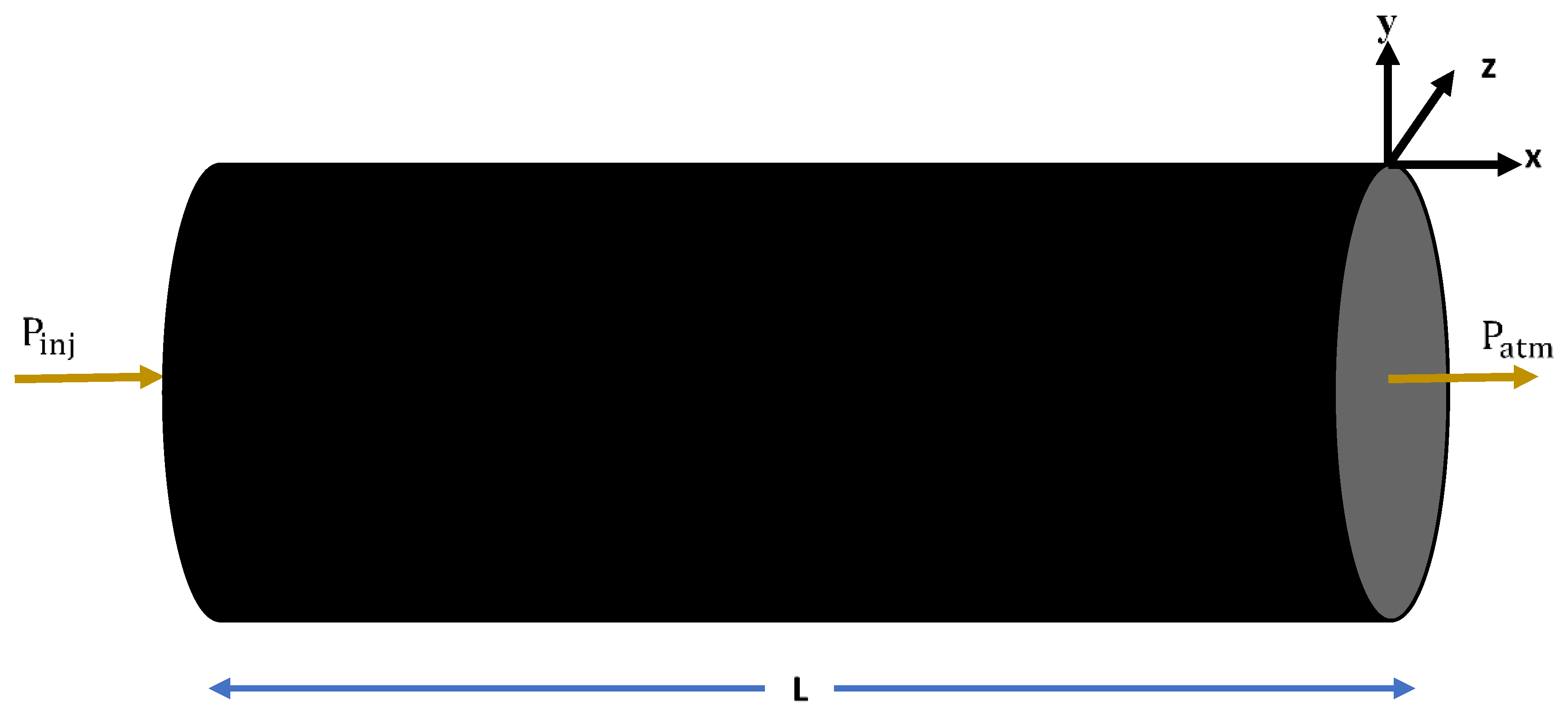
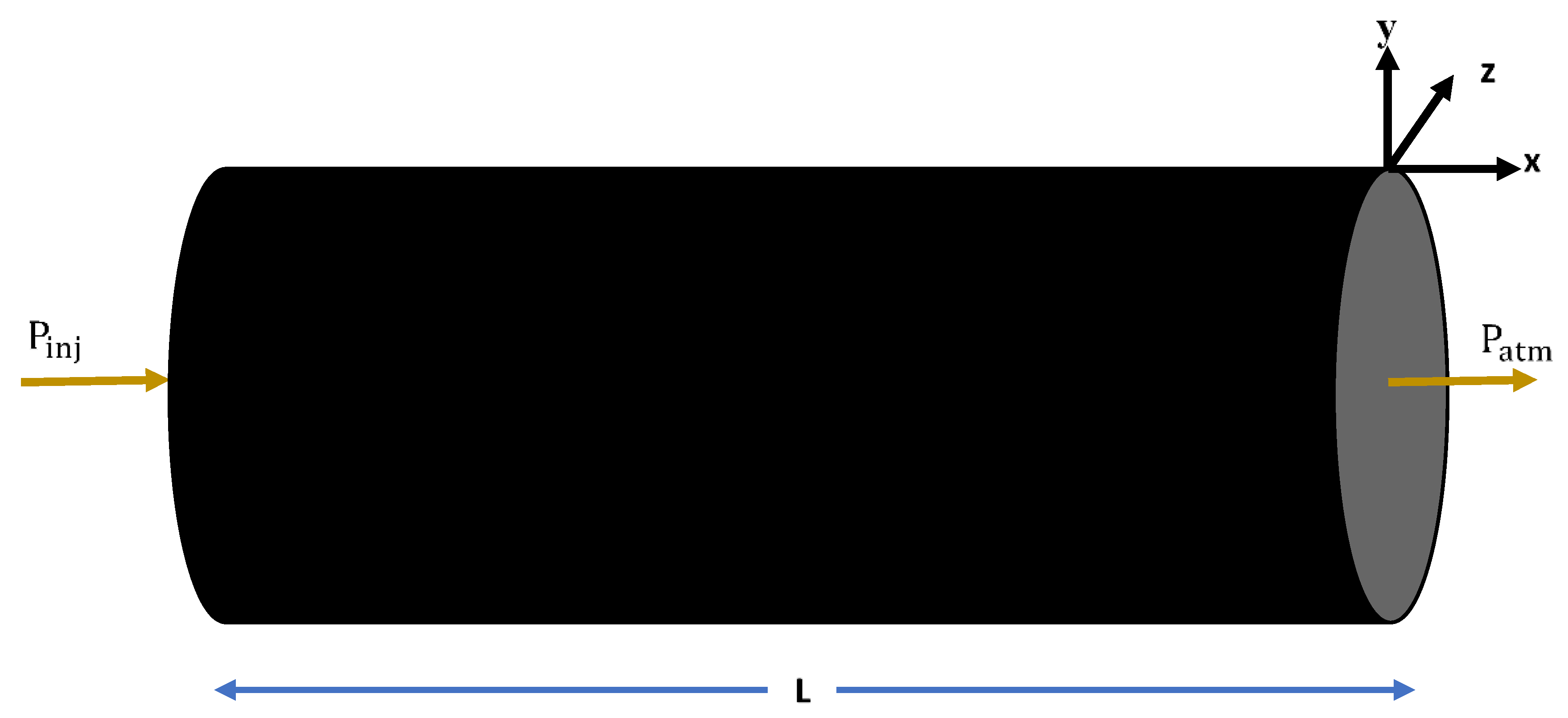
Verification of the proposed mathematical model was performed by deriving analytical solutions for the 1D steady-state and 1D transient gas flow problem depicted in Figure 1, through the simplification of the governing equations described by Equations (1) and (3). In the above problem, flow and deformation can occur only in the longitudinal direction x. A three-dimensional (3D) hydro-mechanical (HM) coupled multiphysics numerical model was built using the commercially available code COMSOL® Multiphysics® (COMSOL®) to solve the simplified governing equations and constitutive relations described below numerically. The analytical solution was then used to verify the numerical model in COMSOL® by comparing the numerical results to the results of the analytical solutions.
The following assumptions were made for the simplification of the mathematical model:
- immobile liquid phase
- no dissolution of gas into and no diffusion gas through the porewater
- constant gas permeability
- constant gas density
- constant fluid viscosity
- constant degree of saturation of water
- role of suction ignored
- role of gravity ignored
- isothermal process
- constant volume boundary condition
It should be noted that these assumptions, as well as the downstream boundary condition set to atmospheric pressure (Figure 1) was done for simplification of the verification analysis. In a bentonite-based shaft seal design, this may be a reasonable assumption when one end of the shaft seal is exposed to surface. However, if applied to bentonite buffer surrounding the waste canister, the boundary pressure conditions would be different and would affect the fluid properties at the higher temperatures and pressures of a DGR environment.
3.2. Analytical Solutions for Two-Phase Flow through a Linear Poro-Elastic Geomaterial
3.2.1. One-Dimensional (1D) Steady-State Gas Flow Problem
Based on the above assumptions, the governing equation for the conservation of gas mass for 1D steady-state flow through a linear elastic porous medium expressed by Equation (11) simplifies to the following expression,
where, is the gas permeability (m2)
Assuming an immobile water phase and ignoring the effects of gravity, the governing equation for the conservation of momentum expressed by Equation (14), simplifies to the following equation for a 1D gas flow problem,
Solving Equation (16), the analytical solution for the pore-gas pressure and displacement as a function of distance can be expressed by,
where is the gas injection pressure (Pa)
- is atmospheric pressure (Pa)
- is the length of the soil specimen (m)
The displacement field along the longitudinal x-direction is given by:
where is the Poisson ratio (unitless)
is Young’s Modulus (Pa)
The corresponding strain and stress can be calculated by the following expressions,
Detailed derivation of the analytical solution for the 1D steady-state gas flow problem is provided in Appendix A.2.
3.2.2. 1D Transient Gas Flow Problem
Based on the assumptions, the governing equation for the conservation of gas mass for 1D transient gas flow through a linear elastic porous medium expressed by Equation (11) simplifies to the following,
By assuming the gas density and degree of saturation remains constant in both time and space, the governing equation for the conservation of momentum expressed by Equation (19) simplifies to the following,
Solving for , this simplifies further to,
Since strain is nil in the y and z directions, it can be shown from Hooke’s Law that
where is the Bulk Modulus (Pa).
Substituting into Equation (25) and re-arranging,
Integrating both sides of the governing equation for the conservation of momentum expressed by Equation (17), and re-arranging for ,
Substituting into Equation (27)
As Equation (29) is analogous to the equation for transient diffusion in a plane sheet, the analytical solution as expressed by J. Crank [25] for constant surface concentrations and constant initial conditions is expressed by the following equation,
where (m2 s−1)
Substituting pg(x,t) from Equation (30) into Equation (28) and then substituting Equation (28) into Equation (26) and integrating both sides, the analytical solution for the displacement can be expressed by,
The strain and stress can now be calculated analytically by the following expressions,
Detailed derivation of the analytical solution for the 1D transient gas flow problem is provided in Appendix A.3.
3.2.3. Mean Stress and Deviatoric Stress
The mean stress can be calculated by the following expression,
The deviatoric stress can be calculated by the following expression,
where,
3.3. Numerical Model Description
Model Geometry and Mesh
For the numerical model, the geometry and mesh are presented in Figure 2. The numerical model consists of approximately 11,000 elements and has 162,000 degrees of freedom.
3.4. Results and Discussion
Verification of the numerical model results against the analytical solution for a 1D steady-state gas flow problem and a 1D transient gas flow problem are presented below. Table 1 provides the material properties, initial conditions, and boundary conditions that were used in both the numerical model and analytical solution. The material properties correspond to those obtained experimentally from Daniels and Harrington [26] or calculated using the constitutive relations derived by Dagher et al. [9]. The initial and boundary conditions were selected based on the experimental setup of Daniels and Harrington [26], with the injection poregas pressure corresponding to the peak injection pressure observed in that experiment.
3.4.1. Steady-State Solution
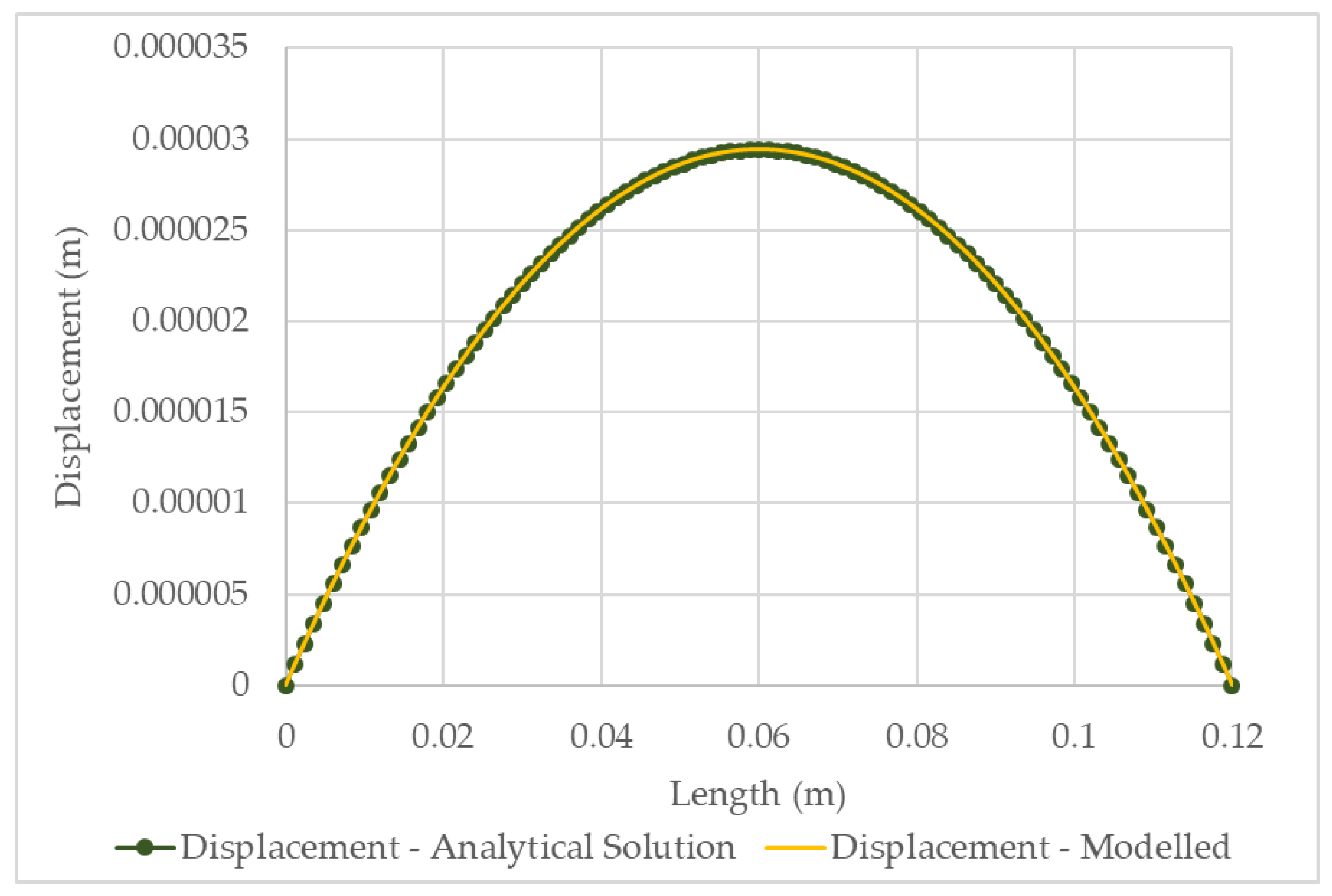
For the 1D steady-state gas flow problem, the poregas pressure and displacement in the x-direction were calculated using analytical solution presented by Equations (18) and (19), respectively. The numerical and analytical results for poregas pressure and displacement over the length of the specimen is provided in Figure 3 and Figure 4, respectively. The results show a perfect match between the simulation results of the numerical model performed in COMSOL® and the analytical solution.
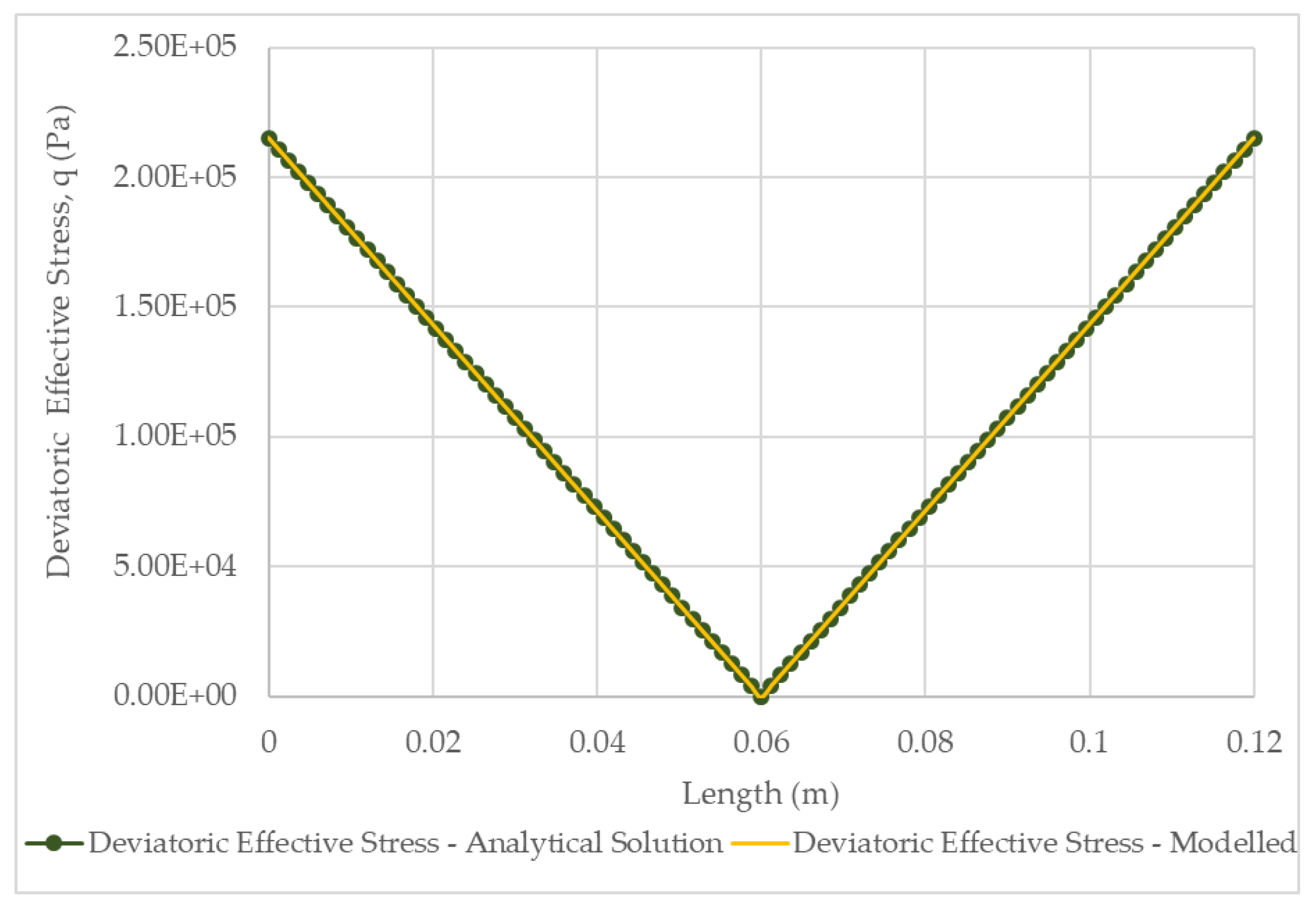
Similarly, the mean effective stress, , and deviatoric effective stress, , were calculated by first calculating the strain and resulting principal stresses described by Equations (20) to (22), and then Equations (33) and (36). The numerical and analytical results for mean effective stress, and deviatoric effective stress over the length of the specimen are provided in Figure 5 and Figure 6, respectively. The results, also show a perfect match between the numerical results performed in COMSOL® and the analytical solution, thereby demonstrating verification of the numerical model being used in COMSOL®.
3.4.2. Transient Solution
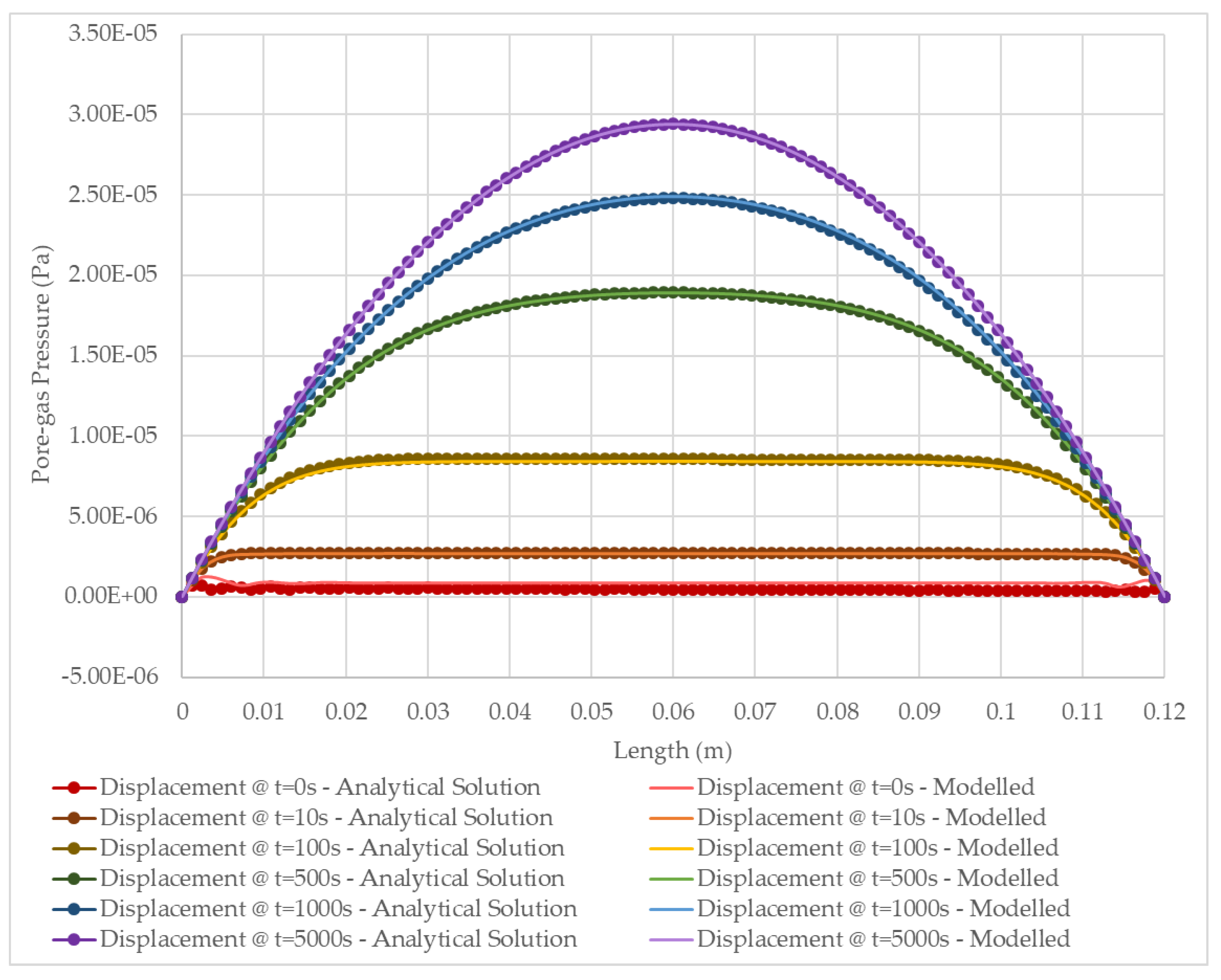
For the 1D transient gas flow problem, the poregas pressure and displacement were calculated using the analytical solution presented by Equations (30) and (31). The numerical and analytical results for poregas pressure and displacement over the length of the specimen for various times are provided in Figure 7 and Figure 8, respectively. The results show a perfect match between the simulation results of the numerical model performed in COMSOL® and the analytical solution. For the poregas pressure, there is an initial response at t = 0 s, corresponding to the sudden change in boundary conditions. Over time, the system tends towards the steady-state solution. Concurrently, as the poregas pressure increases along the column, there is a resulting increase in displacement, until steady-state is reached. Steady-state was achieved at about 5000 s, and matches the solutions provided in Section 3.4.1.
It should be noted that oscillations occurred in results obtained from both the analytical solution and numerical model at time t = 0 s, and this was expected. For the analytical solution, these oscillations are due to truncation of the infinite series at n = 70 and m = 40. As these parameters tend towards infinity, if higher truncation limits were used, the oscillations would effectively dissipate. For the numerical analysis, these oscillations are an artefact of mesh size, time step, and error tolerance. Increasing mesh size, and reducing the time-step and tolerance, would help to reduce the numerical oscillations.
Similarly, the mean effective stress, , and deviatoric effective stress, , were calculated by first calculating the strain described by Equation (32) and resulting principal stresses described by Equations (26) and (22), and then by Equations (33) and (36). The numerical and analytical results for mean effective stress, and deviatoric effective stress over the length of the specimen are provided in Figure 9 and Figure 10, respectively. The results, also show a perfect match between the numerical results performed in COMSOL® and the analytical solution, thereby demonstrating verification of the numerical model being used in COMSOL®.
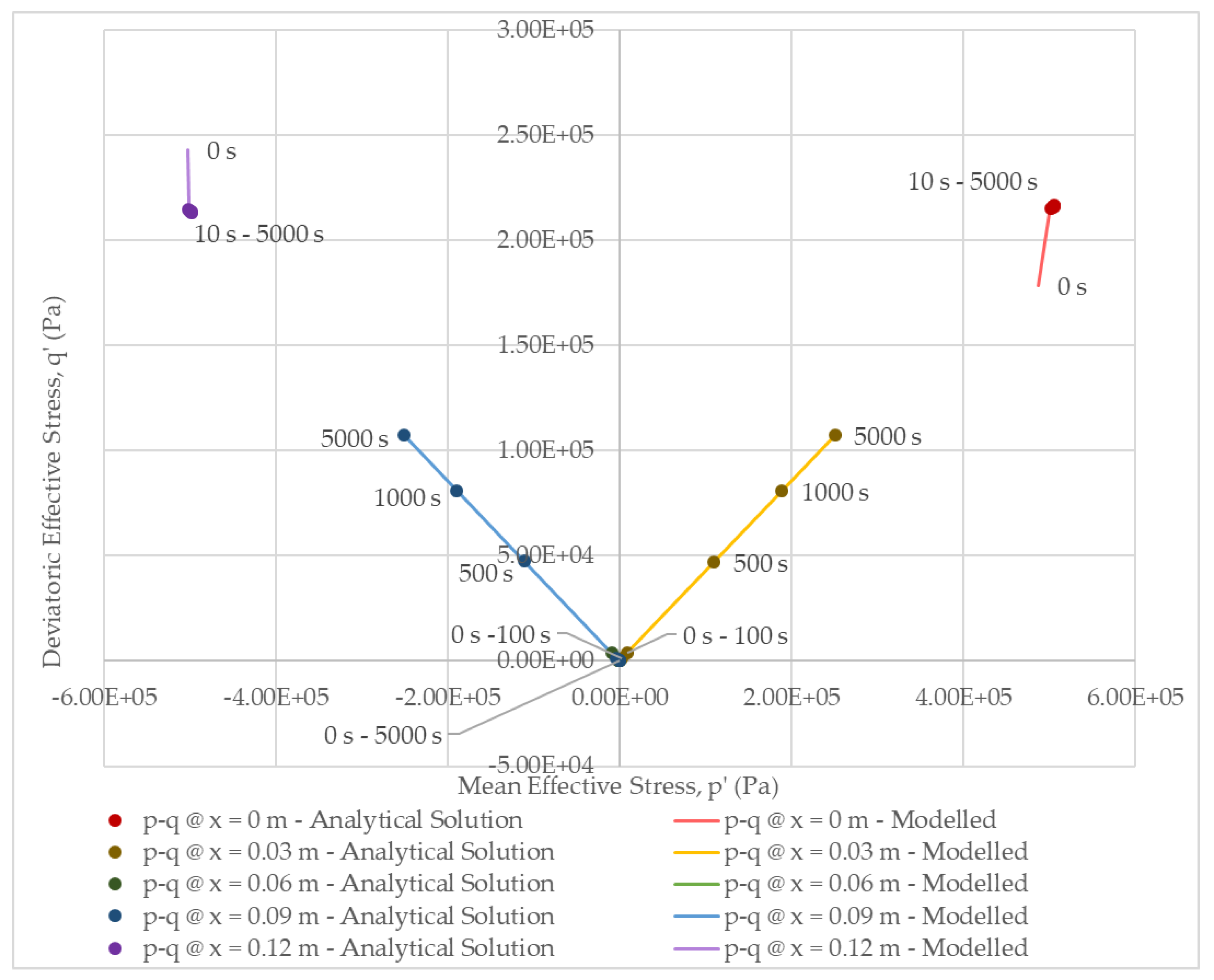
Additionally, an analysis of the p-q stress path at five different points along the specimen over time was conducted and the results are presented in Figure 11. Again, the numerical model results and results of the analytical solution show a close match. The analysis shows that at the center of the specimen, there is no change in stresses as expected. The analysis also shows that at the two ends, there is also no change in stresses as described by the analytical solution, however, the numerical model does show a small change in stress from 0 s to t > 0 s. Again, this can likely be attributed to the truncation of the infinite series. At distances 0.03 m and 0.09 m, the effective deviatoric stress increases linearly as a function of the effective mean stress until steady-state is reached. This is expected as a linear elastic mechanical model was adopted. It should be noted that at the injection pressure side, the mean effective stress is in tension, while at the atmospheric pressure side, the mean effective stress is in compression.
4. Conclusions
An important component in the design and long-term safety assessment of a DGR is the long-term performance of bentonite seals as barriers against gas migration. As gas generates from the degradation of organic waste and/or corrosion of metals, at some critical gas pressure, dilation of the bentonite could occur resulting in the creation of preferential flow pathways and a source of radionuclide exposure to people and the environment. Development and use of numerical models are of key importance in the understanding of processes involved and in their use in long-term safety assessments.
In the authors’ previous work, a fully-coupled hydro-mechanical (HM) linear-elastic mathematical model for advective-diffusive visco-capillary controlled two-phase flow through a geomaterial was derived [9]. This study expands upon that work through the contribution of model verification. As part of this study, analytical solutions for a 1D steady-state gas flow and a 1D transient gas flow problem were derived using the framework of poromechanics. Using the finite element method, the numerical model was used to simulate 1D flow through a confined cylindrical sample of near-saturated low-permeable soil under a constant volume boundary stress condition. Verification of the numerical model was performed by comparing the pore-gas pressure evolution and stress evolution to that of the results of the analytical solutions. For both the steady-state and transient problems, the poregas pressure, displacement, mean effective stress, deviatoric effective stress, and p’-q’ stress path results obtained from the numerical model were compared to those of the analytical solutions. For each parameter, the results of the numerical model closely matched those of the analytical solutions, providing added confidence that the proposed mathematical model is being correctly implemented in the COMSOL® FEM software version 5.4.
Future studies will attempt to improve upon the model complexity and investigate enhanced mechanisms for two-phase flow. In the companion paper, a process simulation and enhanced two-phase flow analysis study will be conducted, whereby three enhanced mechanisms for two-phase flow will be introduced into the model. Specifically, the companion paper will look at heterogeneity, the Klinkenberg “slip flow” effect, and the effect of swelling and dessication. An analysis of the contribution of each to flow behaviour and the potential for the formation of gas fingers will be conducted.
Author Contributions
conceptualization, E.E.D. and T.S.N.; methodology, E.E.D. and T.S.N.; software, E.E.D.; validation, E.E.D., T.S.N. and J.Á.I.S.; formal analysis, E.E.D.; investigation, E.E.D. and T.S.N.; resources, J.Á.I.S.; data curation, E.E.D., T.S.N. and J.Á.I.S.; writing—original draft preparation, E.E.D.; writing—review and editing, T.S.N. and J.Á.I.S.; visualization, E.E.D.; supervision, T.S.N. and J.Á.I.S.; project administration, J.Á.I.S.; funding acquisition, J.Á.I.S. All authors have read and agreed to the published version of the manuscript.
Funding
This work was supported by the Canadian Nuclear Safety Commission.
Acknowledgments
Decovalex (http://www.decovalex.org) is an international research project comprising participants from industry, government and academia focusing on development of understanding, models and codes in complex coupled problems in sub-surface geological and engineering applications. DECOVALEX-2019 is the current phase of the project. The authors appreciate and thank the DECOVALEX-2019 funding organizations, Andra, BGR/UFZ, CNSC, US DOE, ENSI, JAEA, IRSN, KAERI, NWMO, RWM, SÚRAO, SSM and Taipower, for their financial and technical support of the work described in this paper. The statements made in the paper are, however, solely those of the authors and do not necessarily reflect those of the funding organizations.
Conflicts of Interest
The authors declare no conflict of interest.
Appendix A. Analytical Solutions for 1-Dimensional Gas Flow in a Linear Elastic Porous Media
A.1. Problem Statement
Derive the steady-state and transient solutions for 1D gas flow through a linear elastic porous media of length L, fixed at both ends, u(0,t) and u(L,t) = 0, with an initial uniform poregas pressure, pg(x,0) = p0, and with both maintained at different constant gas pressures, pg(0,t) = pinj and pg(L,t) = patm,
Figure A1.
One-dimensional (1D) gas flow through a porous media of length, L.
The following assumptions were made for the simplification of the mathematical model:
- immobile liquid phase
- no dissolution of gas into and no diffusion gas through the porewater
- constant gas permeability
- constant gas density
- constant degree of saturation of water
- role of suction ignored
- role of gravity ignored
- isothermal process
- constant volume boundary condition
A.2. Steady-State Solution
A.2.1. Governing Equations
The governing equation for the conservation of gas mass for steady-state flow through a linear elastic porous medium can be expressed by Equation (A1),
The governing equation for the conservation of momentum (quasi-static equilibrium) for steady-state gas-flow through a linear elastic porous media can be expressed by Equation (A2),
Assuming an immobile water phase, this simplifies to Equation (A3),
A.2.2. Formulation of the Analytical Solution to the Conservation of Mass Equation
Re-arranging Equation (A1) and solving the double integral for pg,
From our known boundary conditions, at , and we can solve for
Substituting (A6) back into (A5) and from our known BCs at , , we can solve for
Substituting Equations (A6) and (A7) into Equation (A5), the analytical solution for the governing equation for the conservation of momentum can be expressed by Equation (A8)
A.2.3. Formulation of the Analytical Solution to the Conservation of Momentum Equation
From Hooke’s Law the normal principal strains and shear strains are provided in Equations (A9) to (A11), and Equations (A12) to (A14) respectively,
For the 1D flow problem, and = 0; and ; and and , these equations reduce to the following,
Re-arranging Equations (A16) and (A17),
Equating Equation (A21) and Equation (A22),
Substituting Equation (A26) into Equation (A21) and re-arranging for as a function of ,
Substituting (A27) and (A26) into Equation (A15), we can solve for ,
Re-arranging in terms of ,
where for a 1D flow problem, it can be shown from Hooke’s Law that
and the Bulk modulus for 1D flow problem, , can be expressed as,
Substituting (A4) and (A31) into (A3) yields,
Re-arranging,
Solving the double integral,
From our known BCs, at , and we can solve for
From our known BCs, , and we can solve for
Substituting Equations (A38) and (A39) into Equation (A37), the analytical solution for the governing equation for the conservation of momentum can be expressed by Equation (A40) and simplified further to Equation (A41)
A.2.4. Final Analytical Solution
The final analytical solution for 1D steady-state gas flow through a linear elastic porous media can be expressed by Equations (A42) and (A43),
The strain and stress can now be calculated analytically by the following expressions,
A.3. Analytical Solution for 1-Dimensional Transient Gas Flow in a Linear Elastic Porous Media
A.3.1 Governing Equations
The governing equation for the conservation of gas mass for transient (i.e., time-dependent) flow through a linear elastic porous medium can be expressed by Equation (A47),
By assuming the gas density and degree of saturation remains constant Equation (A47) simplifies to Equation (A48),
and solving for , this simplifies further to,
Substituting Equation (A32) into Equation (A50), yields
The governing equation for the conservation of momentum (quasi-static equilibrium) for steady-state gas-flow through a linear elastic porous media assuming an immobile water phase was previously described by Equation (A52) as,
Integrating both sides and re-arranging for ,
Substituting Equation (A53) back into Equation (A51)
where
A.3.2 Formulation of the Analytical Solution to the Conservation of Mass Equation
The form of Equation (A53) is analogous to that of non-steady state diffusion in a plane sheet presented in Crank [25]. The analytical solution for non-steady state diffusion in a plane sheet as derived by Crank [25] for constant surface concentrations and constant initial conditions is expressed by the following equation,
where is the concentration at a given distance, , and time, , along the plane sheet
- C1 is the concentration at boundary x = 0
- C2 is the concentration at boundary x = L
- C0 is the initial uniform concentration
Considering our boundary and initial conditions provided in the problem statement.
A.3.3 Formulation of the Analytical Solution to the Conservation of Momentum Equation
Substituting Equation (A55) into Equation (A32), the volumetric strain can be expressed as,
Integrating both sides yields,
From our boundary conditions
Substituting back into Equation (A62), yields,
From our boundary conditions
Substituting back into Equation (A62)
A.3.4. Final Analytical Solution
The final analytical solution for 1D transient gas flow through a linear elastic porous media can be expressed by Equations (A73) and (A74),
The strain and stress can now be calculated analytically by the following expressions,
References
- CNSC. Regulatory Guide G-320, Assessing the Long Term Safety of Radioactive Waste Management; CNSC: Ottawa, ON, Canada, 2006.
- Norris, S. EC FORGE project: Updated consideration of gas generation and migration in the safety case. In Gas Generation and Migration in Deep Geological Radioactive Waste Repositories; Shaw, R.P., Ed.; Geological Society: London, UK, 2015; Special Publications; Volume 415, pp. 241–258. [Google Scholar]
- Shaw, R.P. The Fate of Repository Gases (FORGE) project. In Gas Generation and Migration in Deep Geological Radioactive Waste Repositories; Shaw, R.P., Ed.; Geological Society: London, UK, 2015; Special Publications, 415; pp. 1–7. [Google Scholar]
- Cuss, R.; Harrington, J.; Giot, R.; Auvray, C. Experimental observations of mechanical dilation at the onset of gas flow in Callovo-Oxfordian claystone. In Clays in Natural and Engineered Barriers for Radioactive Waste Confinement; Norris, S., Bruno, J., Cathelineau, M., Delage, P., Fairhurst, C., Gaucher, E.C., Höhn, E.H., Kalinichev, A., Lalieux, P., Sellin, P., Eds.; Geological Society: London, UK, 2014; Volume 400, pp. 507–519. [Google Scholar]
- Ahusborde, E.; Amaziane, B.; Jurak, M. Three-dimensional numerical simulation by upscaling of gas migration through engineered and geological barriers for a deep repository for radioactive waste. In Gas Generation and Migration in Deep Geological Radioactive Waste Repositories; Shaw, R.P., Ed.; Geological Society: London, UK, 2015; Special Publication, 415; pp. 123–141. [Google Scholar]
- Horseman, S.T.; Harrington, J.F.; Sellin, P. Gas migration in clay barriers. Eng. Geol. 1999, 54, 139–149. [Google Scholar] [CrossRef]
- Sellin, P.; Leupin, O.X. The use of Clay as an Engineered Barrier in Radioactive-Waste Management—A Review. Clays Clay Miner. 2013, 61, 477–498. [Google Scholar] [CrossRef]
- Sellin, P. Experiments and Modelling on the behaviour of EBS. Reprot D 2014, 3, 38. [Google Scholar]
- Dagher, E.E.; Nguyen, T.S.; Sedano, J.A.I. Development of a mathematical model for gas migration (two-phase flow) in natural and engineered barriers for radioactive waste disposal. In Multiple Roles of Clays in Radioactive Waste Confinement; Norris, S., Neeft, E., van Geet, M., Eds.; Geological Society: London, UK, 2018; Special Publications. [Google Scholar]
- Nash, P.J.; Swift, B.T.; Goodfield, M.; Rodwell, W.R. Modelling Gas Migration in Compacted Bentonite: A Report Produced for the GAMBIT Club; POSIVA: Helsinki, Finland, 1998. [Google Scholar]
- Hoch, R.; Cliffe, K.A.; Swift, B.T.; Rodwell, W.R. Modelling Gas Migrationin Compacted Bentonite: GAMBIT Club Phase 3 Final Report; POSIVA: Olkiluoto, Finland, 2004. [Google Scholar]
- Fall, M.; Nasir, O.; Nguyen, T. A coupled hydro-mechanical model for simulation of gas migration in host sedimentary rocks for nuclear waste repositories. Eng. Geol. 2014, 176, 24–44. [Google Scholar] [CrossRef] [Green Version]
- Harrington, J.F.; Horseman, S.T. Gas transport properties of clays and mudrocks. In Muds and Mudstones: Physical and Fluid Flow Properties; Aplin, A.C., Fleet, A.J., MacQuaker, J.H., Eds.; The Geological Society of London: London, UK, 1999; Volume 158, pp. 107–124. [Google Scholar]
- Horseman, S.T.; Harrington, J.F.; Sellin, P. Water and Gas Movement in Mx80 Bentonite Buffer Clay. Symposium on the Scientific Basis for Nuclear Waste Management XXVII (Kalmar). Mater. Res. Soc. 2003, 807, 715–720. [Google Scholar] [CrossRef]
- Harrington, J.F.; de la Vaissiére, R.; Noy, D.J.; Cuss, R.J.; Talandier, J. Gas flow in Callovo-Oxfordian claystone (COx): results from laboratory and field-scale measurements. Mineral. Mag. 2012, 76, 3303–3318. [Google Scholar] [CrossRef] [Green Version]
- Graham, C.C.; Harrington, J.F.; Cuss, R.J.; Sellin, P. Gas migration experiments in bentonite: implications for numerical modelling. Mineral. Mag. 2012, 76, 3279–3292. [Google Scholar] [CrossRef] [Green Version]
- Bennett, D.P.; Cuss, R.J.; Vardon, P.J.; Harrington, J.F.; Sedighi, M.; Thomas, R.H. Exploratory data analysis of the Large Scale Gas Injection Test (Lasgit) dataset, focusing on ’second-order’ events around macro-scale gas flows. In Gas Generation and Migration in Deep Geological Radioactive Waste Repositories; Shaw, R.P., Ed.; Geological Society: London, UK, 2015; Special Publications, 415; pp. 225–239. [Google Scholar]
- Marschall, P.; Horseman, S.; Gimmi, T. Characterisation of Gas Transport Properties of the Opalinus Clay, a Potential Host Rock Formation for Radioactive Waste Disposal. Oil Gas Sci. Technol. Rev. IFP 2005, 60, 121–139. [Google Scholar] [CrossRef] [Green Version]
- Khalili, N.; Khabbaz, M.H. A unique relatiship for χ for the determination of the shear strength of unsaturated soils. Géotechnique 1998, 48, 681–687. [Google Scholar] [CrossRef]
- Nguyen, T.; Le, A. Simultaneous gas and water flow in a damage-susceptible bedded argillaceous rock. Can. Geotech. J. 2015, 52, 18–32. [Google Scholar] [CrossRef]
- Huang, S.; Barbour, S.L.; Fredlund, D.G. Development and verification of a coefficient of permeability function for a deformable unsaturated soil. Candian Geotech. J. 1998, 35, 411–425. [Google Scholar] [CrossRef]
- Ho, C.K.; Webb, S.W. (Eds.) Gas Transport in Porous Media; Springer: Dordrecht, The Netherlands, 2006. [Google Scholar]
- Pall, R.; Moshenin, N.N. Permeability of Porous Media as a Function of Porosity and Particle Size Distribution. Trans. Asae 1980, 23, 742–745. [Google Scholar] [CrossRef]
- Carman, P.C. Flow of Gases Through Porous Media; Academic Press Inc.: New York, NY, USA, 1956. [Google Scholar]
- Crank, J. The Mathematics of Diffusion, 2nd ed.; Clarendon Press: Oxford, UK, 1975. [Google Scholar]
- Daniels, K.A.; Harrington, J.F. The Response of Compact Bentonite during a 1D Gas. Flow Test., British Geological Survey Open Report, OR/17/067; British Geological Survey: Nottingham, UK, 2017. [Google Scholar]
Figure 1.
One-dimensional (1D) gas flow through a porous media of length, L.

Figure 2.
Verification study–numerical model (a) geometry and (b) mesh.
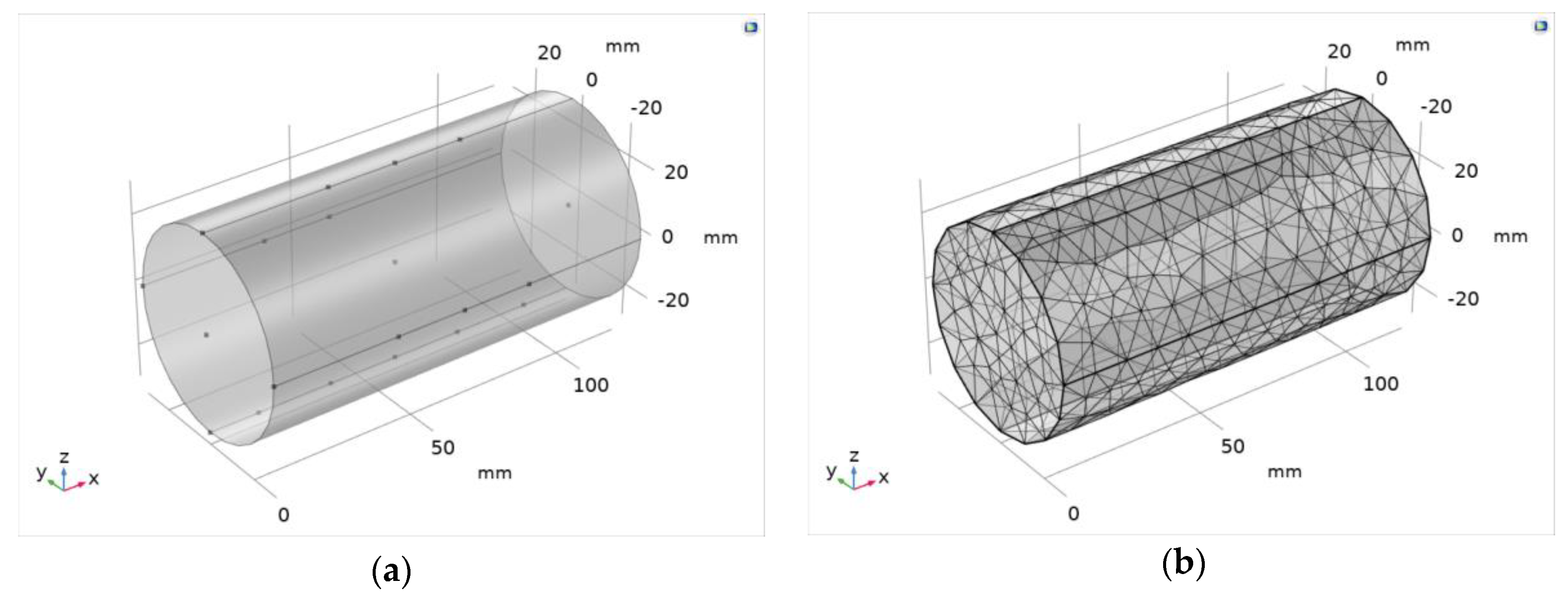
Figure 3.
Verification study—1D steady-state solution results for poregas pressure over the length of the specimen.
Figure 3.
Verification study—1D steady-state solution results for poregas pressure over the length of the specimen.
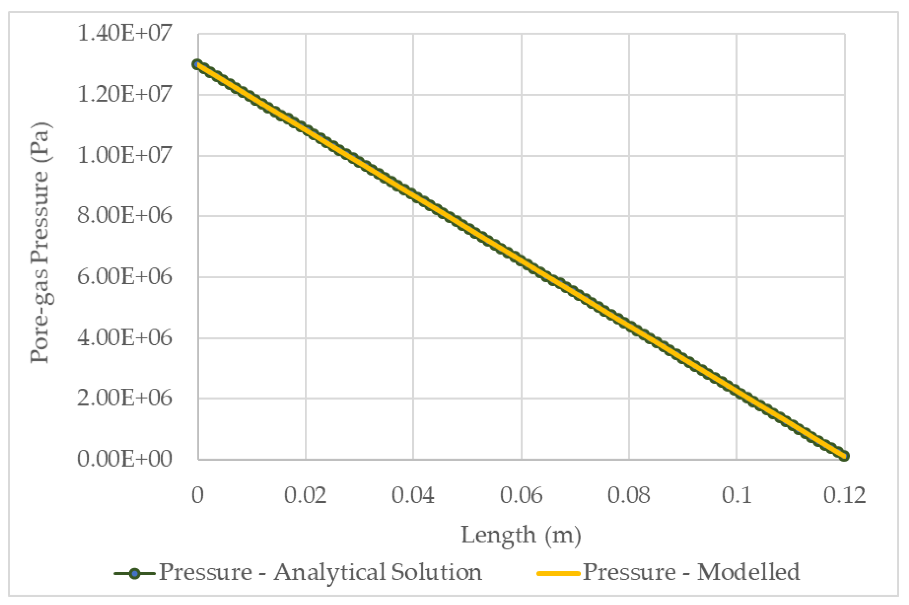
Figure 4.
Verification study—1D steady-state solution results for displacement over the length of the specimen.
Figure 4.
Verification study—1D steady-state solution results for displacement over the length of the specimen.

Figure 5.
Verification study—1D steady-state solution results for mean effective stress over the length of the specimen.
Figure 5.
Verification study—1D steady-state solution results for mean effective stress over the length of the specimen.

Figure 6.
Verification study—1D steady-state solution results for deviatoric effective stress, over the length of the specimen.
Figure 6.
Verification study—1D steady-state solution results for deviatoric effective stress, over the length of the specimen.

Figure 7.
Verification study—1D transient solution results for poregas pressure and over the length of the specimen.
Figure 7.
Verification study—1D transient solution results for poregas pressure and over the length of the specimen.

Figure 8.
Verification study—1D transient solution results for displacement over the length of the specimen.
Figure 8.
Verification study—1D transient solution results for displacement over the length of the specimen.

Figure 9.
Verification study—1D transient solution results for mean effective stress over the length of the specimen.
Figure 9.
Verification study—1D transient solution results for mean effective stress over the length of the specimen.
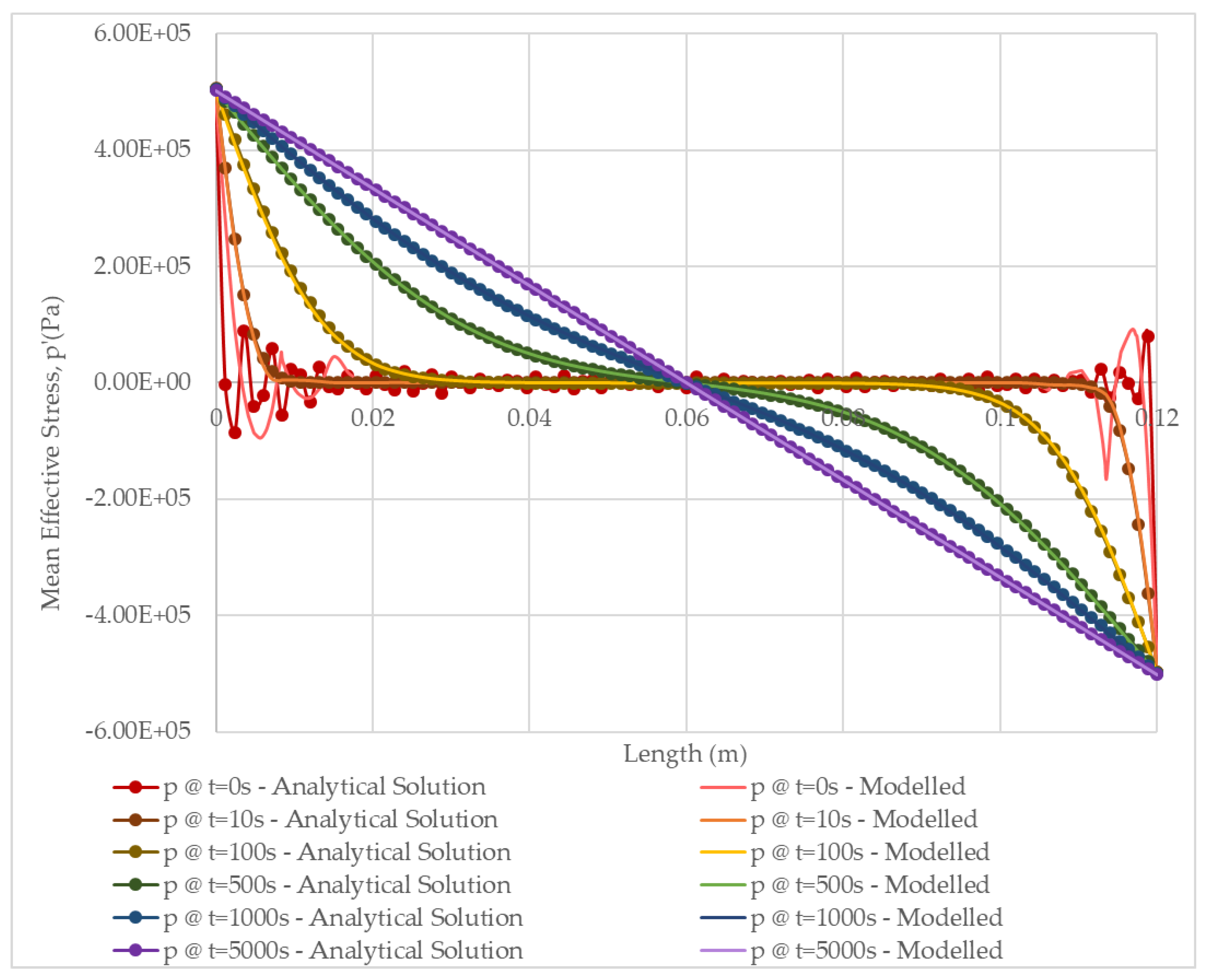
Figure 10.
Verification study—1D transient solution results for deviatoric effective stress over the length of the specimen.
Figure 10.
Verification study—1D transient solution results for deviatoric effective stress over the length of the specimen.
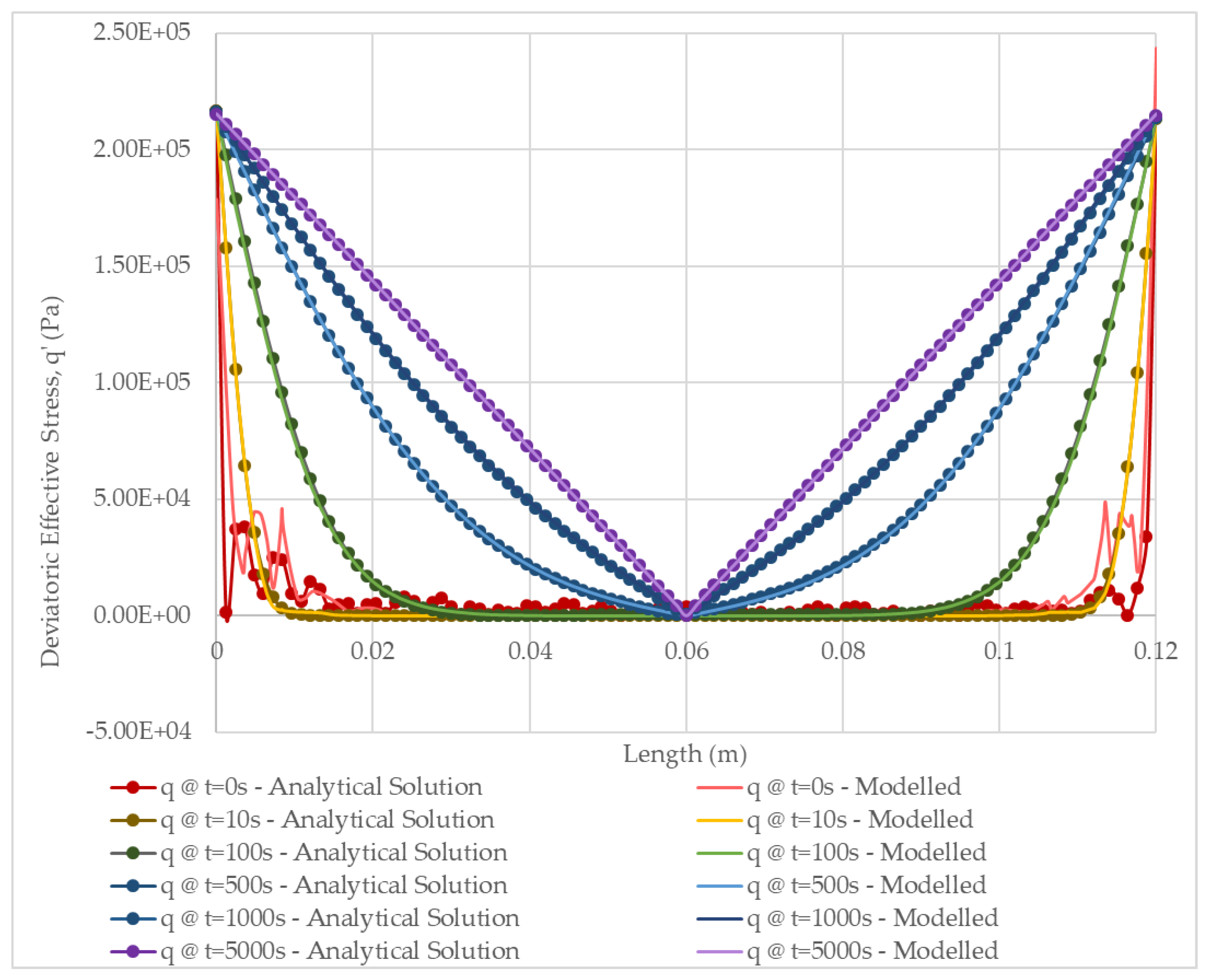
Figure 11.
Verification study—1D transient solution results showing the p-q stress paths along the length of the soil specimen.
Figure 11.
Verification study—1D transient solution results showing the p-q stress paths along the length of the soil specimen.


Table 1.
Verification study parameters.
| Parameter Name | Symbol | Value | Units |
|---|---|---|---|
| Length | 0.12 | m | |
| Injection poregas pressure boundary condition | 1.30 × 10⁷ | Pa | |
| Atmospheric gas pressure boundary condition | 1.01 × 10⁵ | Pa | |
| Initial uniform pore-gas pressure (for transient gas flow problem) | 6.55 × 10⁶ | Pa | |
| Density of bentonite | 1526 | kg m−3 | |
| Young’s Modulus | 3.07 × 10⁸ | Pa | |
| Poisson’s ratio (nu) | 0.4 | - | |
| Porosity | 0.44 | - | |
| Intrinsic permeability | 3.40 × 10⁻²¹ | m2 | |
| Dynamic viscosity | 2.00 × 10⁻⁵ | Pa s | |
| Degree of saturation | 0.9 | - | |
| Air-entry value | 1 × 10⁷ | Pa | |
| Constant porewater pressure 1 | 1.0 × 10⁶ | Pa | |
| Relative gas permeability 1 | 0.03 | - | |
| Chi factor 1 | 0.9 | - |
1 Calculated based on a degree of saturation of 0.9 and gas pressure of 1.3 × 10⁷ Pa.
© 2019 by the authors. Licensee MDPI, Basel, Switzerland. This article is an open access article distributed under the terms and conditions of the Creative Commons Attribution (CC BY) license (http://creativecommons.org/licenses/by/4.0/).
Share and Cite
MDPI and ACS Style
Dagher, E.E.; Infante Sedano, J.Á.; Nguyen, T.S. A Mathematical Model of Gas and Water Flow in a Swelling Geomaterial—Part 1. Verification with Analytical Solution. Minerals 2020, 10, 30. https://doi.org/10.3390/min10010030
AMA Style
Dagher EE, Infante Sedano JÁ, Nguyen TS. A Mathematical Model of Gas and Water Flow in a Swelling Geomaterial—Part 1. Verification with Analytical Solution. Minerals. 2020; 10(1):30. https://doi.org/10.3390/min10010030
Chicago/Turabian StyleDagher, Elias Ernest, Julio Ángel Infante Sedano, and Thanh Son Nguyen. 2020. "A Mathematical Model of Gas and Water Flow in a Swelling Geomaterial—Part 1. Verification with Analytical Solution" Minerals 10, no. 1: 30. https://doi.org/10.3390/min10010030
Note that from the first issue of 2016, this journal uses article numbers instead of page numbers. See further details here.