Uncertainty and Sensitivity Analysis at Low Value of Determination Coefficient of Regression Analysis: Case of I-129 Release from RBMK-1500 SNF under Disposal Conditions

Abstract

As in other nuclear countries, the operation of the Ignalina nuclear power plant in Lithuania has led to the accumulation of around 22 thousand assemblies of spent nuclear fuel (SNF). The development of geological disposal program involves an iterative assessment of the system safety supported by scientific research on radionuclides migration and related processes. This study focused on the application of Contribution to the Sample Mean (CSM) and Contribution to Sample Variance (CSV) methods to complement the uncertainty and sensitivity analyses of the time-dependent flux of I-129 from the engineered barriers of a conceptual disposal facility for RBMK-1500 SNF (RBMK is abbreviation of “High Power Channel-type Reactor” (in Russian)). The analysis was performed using a MATLAB platform (8.0.0.783 (R2012b), MathWorks, MA, USA). The mean and variance ratios derived from CSM and CSV plots were applied to estimate the effect of reduced uncertainty range on mean flux and its variance, and the uncertainty analysis was also complimented. Increasing the lower bounding value of defect size enlargement time range to 4.6 × 10⁴ years would lead to a lower mean flux until 5 × 10⁴ years after repository closure. Later on (up to 1 million years after repository closure), the only reduction of the upper bounding value of the SNF dissolution rate range would affect a decreased mean flux.

1. Introduction

As in other nuclear countries, the operation of the Ignalina nuclear power plant in Lithuania has led to the accumulation of around 22 thousand assemblies of spent nuclear fuel (SNF). Each country’s responsibility for the safe management of its SNF is acknowledged worldwide. Within the European Union (EU), directive 2011/70/EURATOM [1] contains the provision for every member state (country) to be responsible for the implementation of a safe and sustainable solution for SNF and radioactive waste management and disposal.

In the case of SNF disposal, one of the key issues is the demonstration of the long-term safety of the disposal system. Safety assessment covers the understanding and analysis of a broad range of processes in relation to disposal system evolution, radionuclide distribution, and the impact on human health and the environment. Lack of reliable data leads to overestimating environmental impact and modeling results with large uncertainties.

The role of sensitivity analysis (SA) in line with uncertainty analysis (UA) is widely recognized as an effective tool to understand the influence and to rank the most important parameters for reducing uncertainty, i.e., SA helps to determine what parameters most need better determination and to identify those that propagate most variance in the output.

Besides analyzing the relationship between model output and input variables, SA can identify whether a model is over-parameterized [2]. If the uncertainty of a particular parameter does not have any significant impact on the model output being analyzed, its reference (nominal) value could be set, and computational cost reduced. SA methods can be classified in different ways; for example, as graphical methods, mathematical methods, and statistical methods [3]. Mathematical methods are devoted to assessing the impact of the input uncertainty on the model output by performing several simulations typically with a few selected input values. By changing one parameter at a time (OAT), this type of analysis represents local SA. However, previous work has shown the inadequacy of the SA based on OAT, as indicated in [4], with alternatives to OAT presented therein.

Concerning statistical methods, several simulations with input values sampled from their probability distributions need to be performed, and the effect of uncertainty in the input parameters on the uncertainty of model output has been assessed. Examples of statistical methods for parameter ranking include linear regression analysis, regression analysis of rank transformed data, correlation analysis, analysis of variance, response surface methods, the Fourier amplitude sensitivity test (FAST), the extended FAST (EFAST), Sobol indices, etc. Varying the number of input parameters and analyzing the corresponding model results is known as a global sensitivity analysis. It should be mentioned that within the context of geological disposal, the standardized linear regression and correlation analysis are used quite widely [5,6,7,8,9,10,11] for the identification of the most important parameters. Stepwise regression analysis is also used [12,13]. Standardized regression coefficients (SRC), correlation coefficients (Pearson, partial correlation coefficients), and Spearman rank correlation coefficients (SRCC) have been used as the measures of the parameter importance.

Graphical methods assess parameter of importance from graphs, charts, or surfaces (i.e., scatterplots, cobweb plots). Plots of Contribution to the Sample mean (CSM) [14] and Contribution to Sample Variance (CSV) [15] are of the graphical SA type. As indicated in [15], CSV plots provide a considerably higher amount of information than provided by sensitivity indices obtained using global sensitivity methods. Recent applications of CSM and CSV for importance ranking were reported in the studies dealing with a water hammer model [15] and a performance assessment model for a generic high-level waste repository in clay [16]. The CSM method capabilities were tested for a radioactive high-level waste repository in [14]. However, the application of this type of graphical tool for SA within the context of geological disposal is rare.

Up to now, not much research has been done on RBMK type SNF behavior under deep geological repository (DGR) conditions, the potential for contaminant migration, and the subsequent impact on humans and the environment. Some deterministic assessment results were published in [17,18,19]. Radionuclides I-129 and Ra-226 (in the long-term perspective) were identified as dominating the mass flux and radiotoxicity flux from the engineered barrier system (EBS) of DGR under the canister defect scenario. Radionuclides with the largest radiological impact were identified based on the results of mass-transfer analysis and analysis of radiotoxicity flux. The research results showed that depending on the differences in the initial defect size, time of defect size enlargement time, and time when radionuclide release begins, the peak flux from the EBS might vary by a factor of 2 (for I-129) and 1.5 (for Ra-226) for RBMK-1500 SNF [18]. A study [19] analyzed disposal behavior of two types of SNF (Lithuanian RBMK-1500 and Swedish BWR SNF). The comparison of the maximal fluxes from the engineered barriers of the repository showed differences that were not directly proportional to the differences observed in the SNF inventories.

It should be noted that this paper focused entirely on radionuclide transport through EBS. It did not represent safety assessment results for a possible RBMK-1500 SNF DGR, as both the site and the host rock (natural barrier) have yet to be selected. Within the safety assessment, entire disposal system was analyzed, including EBS and surrounding geology and surface environment, and the quantitative assessment was carried out in terms of comparison of modeled dose/risk with dose/risk criteria. However, there are several other indicators, which would be assessed and discussed within the safety case as a complement to dose/risk. These includes performance indicators, such as radionuclide transfer times, radionuclides concentrations in the near field (EBS and part of surrounding host rock), radionuclide fluxes in the near field, characteristics that control “dilution” in time and space (e.g., waste-form dissolution or release rates, canister failure rate), etc. [20].

The most recent results of probabilistic uncertainty and sensitivity analysis of I-129 release through the engineered barriers of a conceptual disposal facility for RBMK-1500 SNF were reported in [21]. In the study [21], the peak flux and the time-dependent flux of I-129 were analyzed as variables of interest (model output), and the importance ranking was performed based on regression/correlation coefficients. Sensitivity measures in terms of standardized regression coefficients (SRC) appeared to be sufficient for importance ranking for peak flux. Meanwhile, for time-dependent flux, it was concluded that regression analysis might not be reliably ranking the parameter importance as the coefficient of determination (R²) became very low (<0.3) 10⁴–10⁵ years after repository closure, indicating strong nonlinearity between the flux and input parameters. For these reasons, this study was devoted to the analysis that would determine the most important parameter for the period where the regression analysis was unreliable.

This study estimated the contribution of each parameter to the mean and variance of model output. Based on derived CSM and CSV plots, the ranking of parameter importance was established for the time-dependent flux of I-129 through the engineered barriers of a conceptual geological repository for RBMK-1500 SNF disposal. It also applied CSM- and CSV-based measures to explore the effect of parameter uncertainty reduction. The effect of reducing the uncertainty of input parameters was assessed in terms of the mean and variance. The advantage of CSM and CSV tools is no necessity of additional model runs. Also, the derivation of complemental results regarding importance ranking was done, where the regression-based method was unreliable, and indications about the effect of newly justified input parameter uncertainty range on the model output were available at no additional computational cost.

1.1. Radionuclide Transport Model for RBMK-1500 SNF Disposal

For studying the long-term performance of a disposal system, commonly involves using numerical models for the analysis of events and processes that take place in (or could affect) the system. There are several processes (thermal, chemical, physical, etc.) influencing the disposal facility (repository) and its surrounding environment necessitating a complex analysis of the processes and their interactions. Thus, the analyzed model output differs from study to study (i.e., peak flux [22], peak time [23], maximum concentration [5], peak dose [24], the amount of radionuclides being released at particular times after repository closure [25], dose over time [26], dose conversion factors [6]). The uncertainty and sensitivity of physical parameters that impact contaminant transport to the environment are considered as a model output to be analyzed (e.g., pressure in the borehole [27]). Nevertheless, the main aim of such studies is to help to assess radionuclide release and migration within the disposal system and its surrounding environment to evaluate the DGR system’s safety.

1.1.1. Disposal System

There is an international consensus that geological disposal facility located at significant depth in stable rock formations offer a reliable and sustainable solution for the long-term management of high-level radioactive waste. The long-term safety of DGRs is ensured by applying the multi-barrier concept. The multi-barrier concept involves the consideration, justification, and implementation of a series of natural (host rocks) and engineered (waste form, package, backfill, and seal materials) barriers [28].

For the disposal of RBMK-1500, SNF in Lithuania DGR constructed in the crystalline rock could be considered. The radionuclide migration is assessed in consideration of engineered barriers, including SNF matrix itself, a copper canister, and surrounding bentonite (Figure 1). More details on the repository concept and radionuclide release model are provided in [21].

The main function of the engineered barrier system of DGR is to prevent and/or limit the release of radionuclides into the surrounding geological environment. As indicated by [29], it is impossible to ensure complete containment for hundreds of thousands of years after repository closure; thus, the eventual release of radionuclides must be minimized after the loss of integrity of the engineered barriers surrounding the SNF matrix. Once the contaminants are released from the engineered barriers, they could be dispersed in the surrounding geological environment and transferred into the biosphere. The main assumptions considered during the assessment of I-129 transfer in the near field region (EBS) were as follows [21]:

• The bentonite material surrounding copper canister will be fully saturated by the groundwater by the time I-129 release from the SNF assemblies;
• As soon as a small initial canister defect becomes large, the void space within the canister (void between SNF assemblies and the channel in the canister insert) will be filled with the groundwater (app. 0.5 m³);
• Mechanisms (instant release of a part of the inventory and congruent release of the rest part of the inventory from degrading SNF matrix) take place in the canister and contribute to the radionuclide flux from the canister;
• Radionuclides released from SNF assemblies interact with a limited amount of water inside the canister, and dissolved radionuclide are transported from the canister in liquid form (mainly by diffusion);
• I-129 is released through the bentonite barrier and diffuses into the water flowing in a (conceptual) fracture intersecting the disposal tunnel.

The selected uncertain input parameters and the properties of the parameter distributions for the probabilistic transport analysis are provided in

Table 1. Summary of input data for the radionuclide release modeling [21].

Parameter	PDF 1			PDF Type
	Nominal Value (Reference Value)	Lower Bound	Upper Bound
Defect size enlargement time (Tlarge) (years) [30]	104	103	105	Triangular
SNF matrix dissolution rate (SNF DR) (1/year) [31]	10−7	10−8	10−6	Triangular
Equivalent groundwater flow rate around the canister (Qeq) (m3/year) [32]	9 × 10−4	9 × 10−4 (p = 0.9)	4 (p = 0.1)	Discrete
Instant release fraction (IRF) of I-129 inventory (%) [31]	2	0	5	Triangular
Effective diffusivity of I-129 in bentonite (De) (m2/s) [33]	1 × 10−11	3 × 10−12 (p = 0.15) 1 × 10−11 (p = 0.7) 3 × 10−11 (p = 0.15)		Discrete

¹ Probability density function. SNF: spent nuclear fuel.

.

1.1.2. Characterization of Model Behavior

The model realized using the computer code AMBER [34] assessed time-dependent radionuclide release from the SNF matrix, dissolution, radioactive decay, and contaminant transport by diffusion through engineered barriers. The uncertainty of the main transport-related parameters, including defect size enlargement time, was characterized by probability density function for each parameter. The model output was a large number of the time-dependent flux values over an extended period (10³–10⁶ years after repository closure), which allowed for the evaluation of the mean flux, the quantiles, and the distribution of the peak flux, as illustrated in Figure 2.

The parameter values were sampled randomly (the Monte Carlo method). In total, 1000 simulations were performed with sampled parameter values. The results of regression analysis (Standardized Rank Regression Coefficient (SRRC) as sensitivity measures) reported in [21] for time-dependent radionuclide flux were the main motivators for the current study and are presented in Figure 3.

Regression model for the analysis of model output dependence on the input parameters is expressed as follows:

$$\frac{\left(y_i-y_m\right)}{S_y}=b_1^{\left(s\right)}\frac{\left(x_1-x_{i,m}\right)}{S_{x_1}}+\dots +b_k^{\left(s\right)}\frac{\left(x_k-x_{i,m}\right)}{S_{x_k}}={\displaystyle \sum }_{i=1}^{k}SRC\left(y,x_i\right)\frac{\left(x_1-x_{i,m}\right)}{S_{x_1}},$$

(1)

$y_m$, $x_{i,m}$ are the average values of model output $Y=(y_1,\dots , y_N$), input parameter $X_i=(x_{1i},\dots , x_{Ni}$), $S_y$, $S_{x_i}$ are respective standard deviations of model output () and input parameter ($X_i$), $b_1^{\left(s\right)}, \dots , b_k^{\left(s\right)}$ are standardized regression coefficients, and N–number of model runs.

SRRC is obtained through regression analysis on rank-transformed data. The rank-transformation is replacement of the original values of the input variables and the model output by their rankings (ranking 1 for the smallest value). This technique is used to linearize monotonic nonlinear relations so that linear regression analysis can be applied to the rank-transformed data [35].

As previously mentioned, the SA of radionuclide migration through the engineered barriers of a conceptual geological repository for RBMK-1500 SNF disposal was performed [21]. The maximal (peak) flux and the time-dependent flux of I-129 were analyzed, and the SA was done based on regression/correlation coefficients. The regression analysis of I-129 peak flux yielded a determination coefficient (R²) of 0.77, showing the relationship between the peak flux of this nuclide and the main transport-related parameters was not strongly linear. However, the standardized regression coefficients could still be used to rank parameter importance. For the peak flux of I-129, the effective diffusion coefficient in bentonite (De) and the instant release fraction (IRF) were found to be the most important input parameters.

Meanwhile, the regression analysis results for the time-dependent flux of iodine indicated that given parameters impact varied with different time steps. Effective diffusivity of I-129 in bentonite (De) and the instant release fraction (IRF) was reported as the most important parameters from 10³–10⁴ years after repository closure. Within 10⁴–10⁵ years after closure, the importance of De and IRF was significantly decreased, and the time when initial defect increases became important. Based on the regression analysis, defect size enlargement time (Tlarge) became the most important parameter after approx. 2 × 10⁴ years after repository closure.

However, R² became very low (<0.3) during this period, indicating strong non-linearity between the flux and the parameters; thus, the regression analysis of the rank-transformed data might not provide reliable results for determining parameter importance.

For these reasons, this study was devoted to the analysis that would determine the most important parameter for the period where the regression analysis was unreliable. The contribution of each parameter uncertainty to the mean and variance of model output was estimated through CSM and CSV plots, and conclusions of parameter importance could be derived then.

2. Methodology/Approach for Extension of Sensitivity Analysis Based on CSM and CSV

2.1. Contribution to Sample Mean (CSM)

The CSM plot was introduced by [7] and further developed by [14]. To create a CSM plot, a random (or quasi-random) sample of size N for inputs Xi and corresponding model outputs Y need to be generated. The dependence (function) for a given input parameter Xi is then derived with the application of the following steps as provided in [14]:

• The randomly (quasi-randomly) generated values of $X_i^{}$ from its probability distribution function (PDF) are sorted in ascending order, generating the series of values $\left\{x_{i,1}^{},x_{i,2}^{},\dots ,x_{i,k}^{},\dots ,x_{i,N}^{}\right\}$, $k=1,\dots ,N$;
• The output values $y_i^{}$ corresponding to sorted input $X_i^{}$ are obtained too $\left\{y_{i,1}^{},y_{i,2}^{},\dots ,y_{i,k}^{},\dots ,y_{i,N}^{}\right\}$, $k=1,\dots ,N$;
• An ancillary variable M_i is calculated, whose values are calculated from $y_{i,q}^{}$ as

  $$m_{i,k}^{}=\frac{1}{N}{\displaystyle \sum _{j=1}^k{y}_{i,j}^{}},k=1,\dots ,N$$

  (2)

  i.e.: $m_{i,1}^{}=\frac{1}{N}{y}_{i,1}^{}$, $m_{i,2}^{}=\frac{1}{N}\left(y_{i,1}^{}+y_{i,2}^{}\right)$, $m_{i,3}^{}=\frac{1}{N}\left(y_{i,1}^{}+y_{i,2}^{}+y_{i,3}^{}\right)$, etc.
• The function $CS{M}_{X_i}^{}$ is obtained by normalization of $M_i^{}$, i.e., dividing the values $m_{i,k}^{}$ by the sample mean of model output $y_m^{}$:

  $$CS{M}_{X_i}^{\left(k\right)}=\frac{m_{i,k}^{}}{y_m},k=1,\dots ,N$$

  (3)
• Cumulative relative frequency (cumulative fraction) of the sorted input parameter $X_i^{}$ lies in the interval [0,1] and could be calculated:

  $$q_{X_i}^{\left(k\right)}=\frac{k}{N},k=1,\dots ,N$$

  (4)
• Then, the function $CS{M}_{X_i}^{\left(k\right)}$ is plotted versus the cumulative relative frequency of $q_{X_i}^{\left(k\right)}$. CSM also lie in the interval [0,1].

Each data point of $q_{X_i}^{\left(k\right)}$ corresponds to a particular value of input parameter value in series $\left\{x_{i,1}^{},x_{i,2}^{},\dots ,x_{i,k}^{},\dots ,x_{i,N}^{}\right\}$ (values sorted in ascending order). Each data point ($q_{X_i}^{\left(k\right)}$, $CS{M}_{X_i}^{\left(k\right)}$) represents the fraction of the output mean due to any given fraction of the values of the input lower than that of corresponding to $q_{X_i}^{\left(k\right)}$ [14]. For example, the fraction of output mean at point ($q_{X_i}^{}$ = 0.25) is determined by the 25% of the lowest values of the parameter $X_i^{}$.

CSM plot allows the contribution to the sample mean of the analyzed output Y to be assessed over a certain range of input parameter $X_i^{}$ values. For example, the impact of 20% of the lowest $X_i^{}$ values on the mean of Y could be analyzed over the range [0,0.2] on the x-axis. The impact on the mean is then assessed from the y-axis. The contribution to the output’s mean could vary along with the range of the input parameter’s values, which is reflected by the CSM curve shape.

The ranking of the most important input parameters with regard to the output mean is based on the greatest distance (D_m) of the CSM plot from the diagonal. The CSM curve could cross the diagonal several times. According to [14], the ranking of parameter importance could be based on the sum of maximum distances (in absolute values) of the CSM curve from the diagonal (D_m).

2.2. Contribution to Sample Variance (CSV)

Contribution to sample variance is an extension of CSM first introduced by [15]. For CSV plot, a random sample of size N for inputs $X_i^{}$ and corresponding model outputs Y must again be generated. The dependency (function) for a given input parameter $X_i^{}$ is obtained using the following steps according to [15]:

• The output mean $y_m^{}$ is computed, and each value of output $Y$ is transformed by subtracting the mean value $y_m^{}$_. The transformed output $Yt$ has zero mean value.
• The randomly (quasi-randomly) generated values of input $X_i^{}$ are sorted in ascending order, generating the series of values $\left\{x_{i,1}^{},x_{i,2}^{},\dots ,x_{i,k}^{},\dots ,x_{i,N}^{}\right\}$, $k=1,\dots ,N$, and the corresponding set of the transformed outputs $y{t}_{i,k}^{}$ is obtained $\left\{y{t}_{i,1}^{},y{t}_{i,2}^{},\dots ,y{t}_{i,k}^{},\dots ,y{t}_{i,N}^{}\right\}$, $k=1,\dots ,N$.
• Function CSV is obtained as follows

  $$CS{V}_{X_i}^{\left(k\right)}=\frac{{\displaystyle \sum _{j=1}^{k}y{t}_{\left(i,j\right)}^2}}{{\displaystyle \sum _{j=1}^{N}y{t}_{\left(i,j\right)}^2}},k=1,\dots ,N$$

  (5)
• Cumulative relative frequency (cumulative fraction) of the sorted input parameter $X_i^{}$ lies in the interval [0,1] and could be calculated by Equation (4).

Then, the function $CS{V}_{X_i}^{}$ is plotted versus the cumulative relative frequency of $q_{X_i}^{}$. CSV also lies in the interval [0,1]). The plot consists of pairs ($q_{X_i}^{\left(k\right)}$, $CS{V}_{X_i}^{\left(k\right)}$) corresponding to each point $x_{i,k}^{}$ of the input parameter $X_i^{}$ (in sorted series).

CSM or CSV curves that plot close to the diagonal indicate that the contribution to the mean or the variance is equal with each value of the input parameter being analyzed. For example, the CSV value at quantile q = 0.1 provides an estimate of the model output variance due to 10% of the smallest values of the input parameter. According to [14], if at some regions of the plot, the CSM (CSV) curve is increasi ng quickly, the contribution to the output mean (variance) is large. Where the CSM (or CSV) curve is flat, this means that the contribution to the output mean (or variance, respectively) will be small.

Besides identifying the most important input, CSM and CSV methods provide insight into which part of the input parameter uncertainty range affects uncertainty in model outputs (its mean and variance).

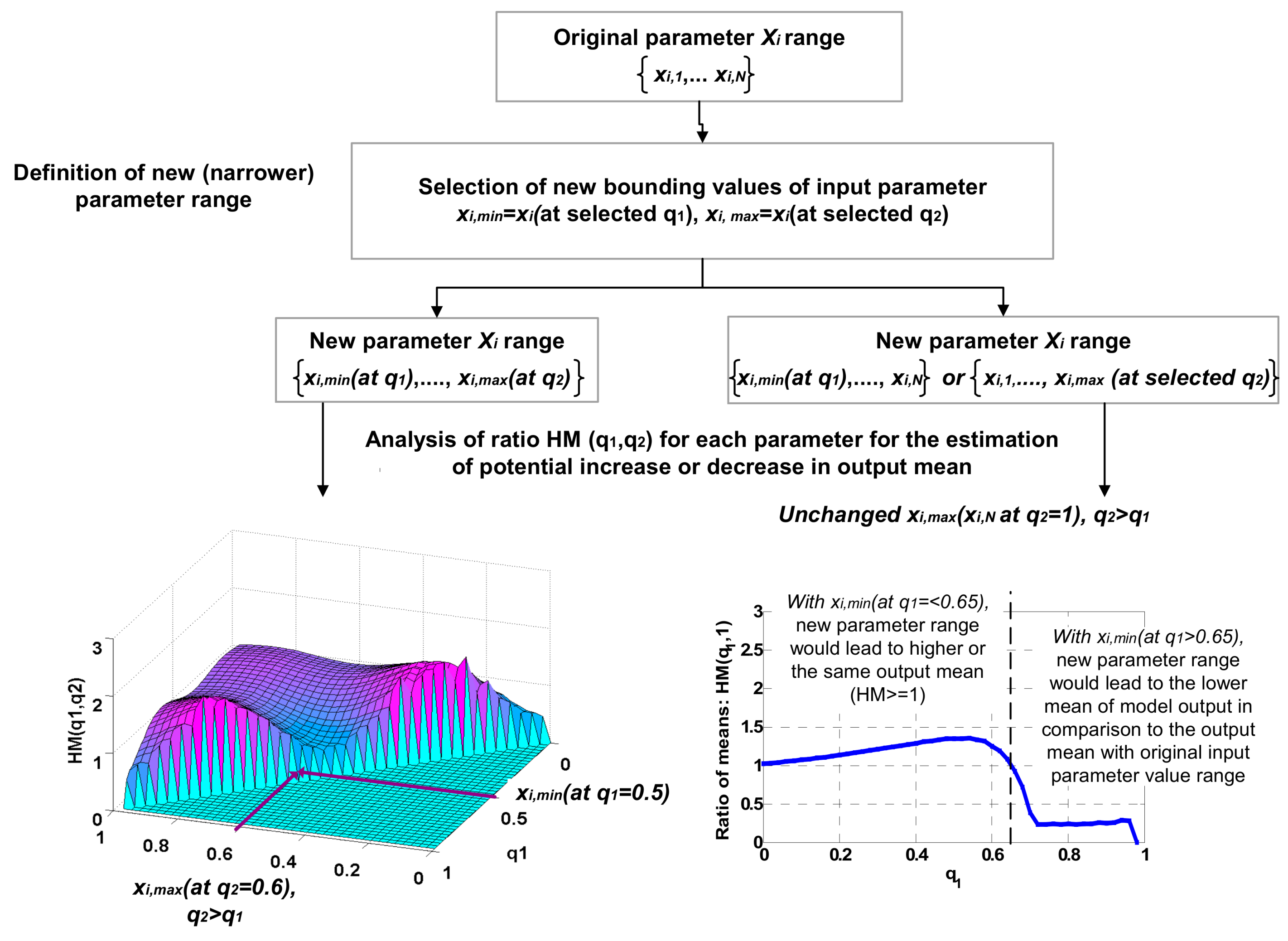
2.3. Revised Mean and Variance Ratio Functions

To complement the UA and SA of I-129 release from the conceptual RBMK-1500 SNF disposal facility, a part of the current study was devoted to getting insights on the effect of parameter uncertainty reduction with application of revised mean and variance ratio functions. Authors of study [36] revised the variance ratio proposed by [15] and introduced revised mean and variance ratio functions (HM and HV, respectively), to be derived as follows:

• The mean $y_m^{}$ of model output $Y$ is computed.
• The generated values of the input X_i are sorted in ascending order, generating the series of values $\left\{x_{i,1}^{},x_{i,2}^{},\dots ,x_{i,k}^{},\dots ,x_{i,N}^{}\right\}$, $k=1,\dots ,N$, and the corresponding set of model output values $\left\{y_{i,1}^{},y_{i,2}^{},\dots ,y_{i,k}^{},\dots ,y_{i,N}^{}\right\}$, $k=1,\dots ,N$ is obtained.
• Cumulative fractions of the input parameter $q_1,q_2$ lying in the interval [0,1] are defined:

  $$q_1,q_2=\frac{k}{N},k=1,\dots ,N_{}$$

  (6)
• The mean ratio function $H{M}_i$ and variance ratio function $H{V}_i$ for $q_1\in [0, 1], q_2\in [0, 1]$ can be estimated by the following expressions

  $$H{M}_i\left(q_1,q_2\right)=\frac{{\displaystyle \sum _{j=q_1}^{q_2}{y}_{\left(i,j\right)}^{}}}{\left(q_2-q_1\right)\cdot {\displaystyle \sum _{j=1}^N{y}_{\left(i,j\right)}^{}}}{,}_{{{\displaystyle }}^{}}0<q_1<q_2,$$

  (7)

  $$H{V}_i\left(q_1,q_2\right)=\frac{CSV{}_i\left(q_2\right)-CSV{}_i\left(q_1\right)}{q_2-q_1}-\frac{y_m^2}{\mathrm{var}\left(Y\right)}{\left(\frac{CS{M}_i\left(q_2\right)-CS{M}_i\left(q_1\right)}{q_2-q_1}-1\right)}^2{,}_{{{\displaystyle }}^{}}0<q_1<q_2$$

  (8)

These ratio functions allow direct observation of change (for example, decrease) of mean and variance of model output due to reduced parameter uncertainty. The effect on model output could be explored on the graph for any pair of selected new q₁ and q₂.

3. Results and Discussion

The results are arranged in three subsections. The extension of SA with the means of derived CSM and CSV plots for I-129 flux is presented first. The second subsection presents the results and discussion about the effect of parameter uncertainty range reduction on the uncertainty of the peak flux in terms of statistical uncertainty measures, such as mean and variance. Finally, the analysis of the effect of parameter uncertainty reduction on the uncertainty of flux over time (in terms of the mean) is presented.

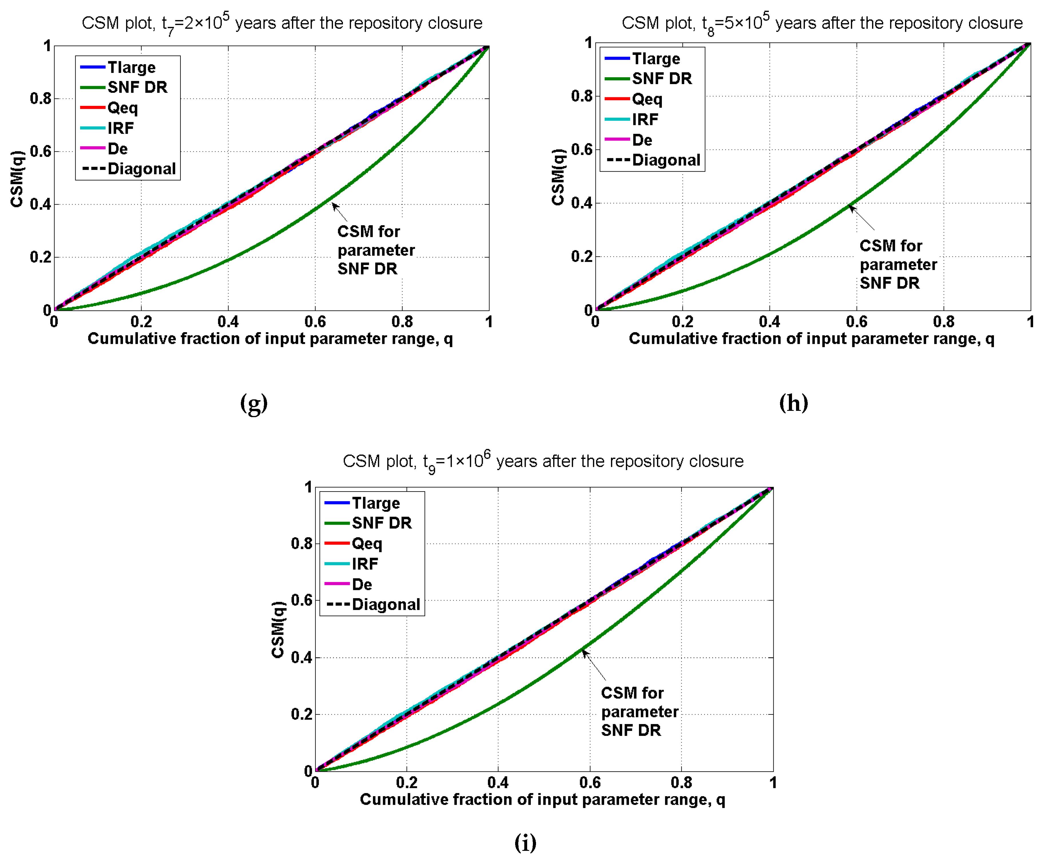
3.1. CSM and CSV Plots for I-129 Flux

For the application of CSM and CSV methods, the language of technical computing MATLAB was employed to derive CSM and CSV plots, mean and variance ratios.

Figure 4 represents the CSM plots of the radionuclide flux from the engineered barrier to the geological barrier at different times up to 1 million years after repository closure (t₁ = 1 × 10³ years; t₂ = 5 × 10³ years, t₃ = 1 × 10⁴ years, t₄ = 2 × 10⁴ years, t₅ = 5 × 10⁴ years, t₆ = 1 × 10⁵ years, t₇ = 2 × 10⁵ years, t₈ = 5 × 10⁵ years, t₉ = 1 × 10⁶ years).

At time t₁ and times t₆–t₉, the most important parameters for the mean flux were clear (the CSM of these parameters had the largest distance from the diagonal D_m): effective diffusivity of I-129 in bentonite (De) was the most important parameter at the very beginning of the release, and the SNF dissolution rate dominated in the long-term. This correlates well with the results of the regression analysis presented in Section 1.1.2.

The CSM plots showed that at certain points in time during between 5 × 10³–5 × 10⁴ years after closure (t₂, t₃, t₄, t₅), the defect size enlargement time was important (see Figure 4). The importance of the defect size enlargement time was observed at earlier points in time (at 5 × 10³ years) in comparison to what was observed from the regression analysis (at 2 × 10⁴ years after the closure). As previously discussed (Section 1.1.2), the coefficient of determination (R²) decreased significantly during this period, and the regression-based ranking was considered as not reliable enough.

The CSM plots where the curve is close to the diagonal (where equivalent groundwater flow rate around the canister (Qeq) and all remaining parameters except for the SNF dissolution rate at 200 thousand years post repository closure) revealed a similar contribution to the mean flux over any quantile range of parameter values. Thus, these parameters could be fixed at any value within the range of the uncertainty without any effect on the mean flux at the corresponding time (Figure 4).

At time t₅ (5 × 10⁴ years, corresponding to the time of maximal mean flux), the most important parameter Tlarge (defect size enlargement time) was confirmed by the maximum distance to the diagonal (D_m(Tlarge) = 0.38), while the SNF dissolution rate and IRF (instant release fraction) were significant though to a lesser extent (D_m(SNF DR) = 0.16, D_m(IRF) = 0.13).

The CSM plots (Figure 4) illustrated a significant variation of the Tlarge curve overt time. The variation represented the uneven contribution of parameter values from the predefined range at different periods. For example, the CSM plot at t₂ = 5 × 10³ years (Figure 4b) showed that 2% of the smallest Tlarge values contributed to almost 36% of the output mean. At t₃ = 1 × 10⁴ years (Figure 4c), ~10% of the smallest Tlarge values contributed to almost 68% of the mean flux. At a later time point t₅ (the observed I-129 mean flux maximum), the greatest values from the range of parameter values played a more important role: ~30% of the greatest Tlarge values contributed to more than 90% of the mean flux.

The actual change of the mean (variance), which could be achieved by reducing the parameter value range to $X_i^{}$ (q₁, q₂) (where q₁ < q₂ < 1), has been presented and discussed in the next sections using revised mean ratio functions.

Figure 5 presents the CSV plots that indicate the influence of each parameter on the flux variance at different time points. The results showed the complexity of the model and varying contribution (of different parameters) to the model output variance over a simulated period (up to 1 million years after repository closure).

At the beginning of radionuclide release from the engineered barriers (t₁ = 1 × 10³ years), the largest contribution to the flux variance came from De (effective diffusivity of I-129 in bentonite), as observed from its curve (Figure 5a). This is similar to what was observed from the CSM plots (regarding the contribution to the mean flux). At later time points, the impact of this parameter was less significant, and the time of defect size enlargement (Tlarge) became the most significant contributor (t₂–t₆, ~5 × 10³–10⁵ years after the repository closure). Based on the CSV plots, parameter Qeq had a more significant influence on variance than on the mean flux up to 5 × 10³ years after repository closure.

Uneven contribution to the variance was observed for the SNF dissolution rate (SNF DR). As for the Tlarge parameter in the CSM plots, the SNF dissolution rate on the CSV plot crossed the diagonal, indicating that the smallest and the largest values of this parameter contributed more to the output variance than the values from the middle part of the quantile range.

Table 2. Significant parameters throughout the analyzed period (up to 1 million years after repository closure).

Time, Years	Most Important Parameters by Regression Analysis [21]	Most Important Parameters by CSM	Most Important Parameters by CSV	Notes
t1 = 1 × 103 years	De, IRF	De, IRF	De	IRF, Qeq are also significant based on CSV
t2 = 5 × 103 years	De, IRF	Tlarge, De, IRF	Tlarge, Qeq, De, IRF	Small Qeq values and De, IRF, are important to some extent
t3 = 104 years	De, IRF, Tlarge	Tlarge, IRF	Tlarge, IRF	The same for both (CSM and CSV) methods
t4 = 2 × 104 years	Tlarge, De	Tlarge	Tlarge	Low importance of SNF DR, De, IRF
t5 = 5 × 104 years	SNF DR, Tlarge	Tlarge, SNF DR, IRF	Tlarge	Ranking of the most important parameter is the same for both (CSM and CSV) methods
t6 = 105 years	SNF DR, Tlarge	SNF DR, Tlarge	Tlarge	Ranking of the most important parameter differs
t7 = 2×105 years	SNF DR	SNF DR	SNF DR	Based on CSM, the rest parameters are non-influential and could be assigned a fixed value without influence on the mean flux for this time. Smallest and largest values of SNF DR are more contributing to flux variance; low importance of Tlarge based on CSV
t8 = 5 × 105 years	SNF DR	SNF DR	SNF DR
t9 = 106 years	SNF DR	SNF DR	SNF DR

Tlarge—defect size enlargement time, SNF DR—SNF matrix dissolution rate, Qeq—equivalent groundwater flow rate around the canister, IRF—instant release fraction, De—effective diffusivity of I-129 in bentonite, CSM—contribution to the sample mean, CSV—contribution to the sample variance.

provides the most significant parameters for time-dependent radionuclide flux into geosphere based on the CSM and CSV plots. In the majority of cases, the ranking for both methods was the same, except for t = 1 × 10⁵ years after closure when the most significant contribution to the mean flux came from SNF DR, and the most significant contribution to flux variance came from Tlarge. The effect of SNF DR on the variance was also observed to be uneven, and the smallest and the largest values of SNF DR contributed most to variance; however, this was not the case for the CSM plot.

3.2. Effect of Parameter Range Reduction on Mean and Variance of I-129 flux

As mentioned above, the derivation of CSM and CVM plots provided an opportunity to assess the range of the input parameter values to focus on to affect the output mean or variance. Several cases were analyzed in terms of analysis of the effect of uncertainty reduction. Cases were devoted to exploring the effect of five parameters’ range reduction:

• on mean I-129 flux at time t = 5 × 10⁴ (peak time),
• on the variance of I-129 flux at time t = 5 × 10⁴ (peak time),
• on mean flux over time.

Additional ways of decreasing the range of parameter values were also considered:

• impact of increasing the lower bounding value and decreasing upper bounding value,
• impact of increasing the lower bounding value while maintaining the original upper bounding value,
• impact of decreasing the upper bounding value while maintaining the original lower bounding value.

3D mean (variance) ratio HM (HV) plots enable the assessment of any effect on the mean (variance) for a range of parameter values $X_i^{}$ (at q₁, at q₂), satisfying the condition q₁ ≤ q₂ (see Section 2.3 for definition).

Scheme for the exploration of the effect of the input parameters uncertainty reduction on model output with the means of ratio HM for each parameter (while keeping the other parameters at their original ranges) is presented in Figure 6. The same procedure is valid in the case of HV.

Figure 7a–e present the 3D plots of the revised mean ratio (HM) for all parameters at t₅ = 5 × 10⁴ years corresponding to the time of maximal mean flux. As the plots demonstrate, for defining reduced ranges for parameter $X_i^{}$ values (with assignment of the new lowest value of the range to be equal to value at selected q₁ and the highest value to be equal to value at selected q₂), the change of new mean (variance) could be estimated from the ratio HM (HV). If the ratio is >1, then the new estimate would be higher than that observed with the original parameter uncertainty range. If the ratio is <1, then the mean (variance) of the model output with a reduced parameter uncertainty range would be lower in comparison to the original one.

As follows from Figure 7, increasing the minimal value of parameter Tlarge to be equal to q₁ > 0.7 and the decrease of the maximal value to be equal to q₂ ≥ q₁ would result in significant mean reduction (HM < 1). But assigning the Tlarge values at q₁~q₂~0.65 would result in increasing the mean by a factor of ~6. The 3D plot of HM(q₁, q₂) over q₁ and q₂ for the parameter SNF DR (Figure 7b) showed a trend leading to an increased mean by a factor of ~3, in the case of a significant increase in the lower bounding value (assigning it equal to value at q₁ between 0.7 and 1). For the same parameter, decreasing the upper bound and increasing of the lower bound, a decrease in the mean flux would be expected. A similar trend was observed for instant release fraction (IRF). The effect of decreased mean due to the reduction of parameter uncertainty range was very limited for parameters Qeq and De (HM around 1).

Figure 8 presents the 3D plots of the revised variance ratio (HV) for all parameters at t₅ = 5 × 10⁴ years (corresponding to the time of maximal mean flux).

From the plots in Figure 8, the effect of changing the parameter uncertainty range on the flux variance is observable. The reduction of uncertainty of Tlarge values to a certain range would lead to a significant decrease in the flux variance. But the plot also showed the presence of a parameter range that would lead to the increased flux variance.

For ease of interpretation, the change in the parameter value range was explored in 2D plots derived from the 3D plots above.

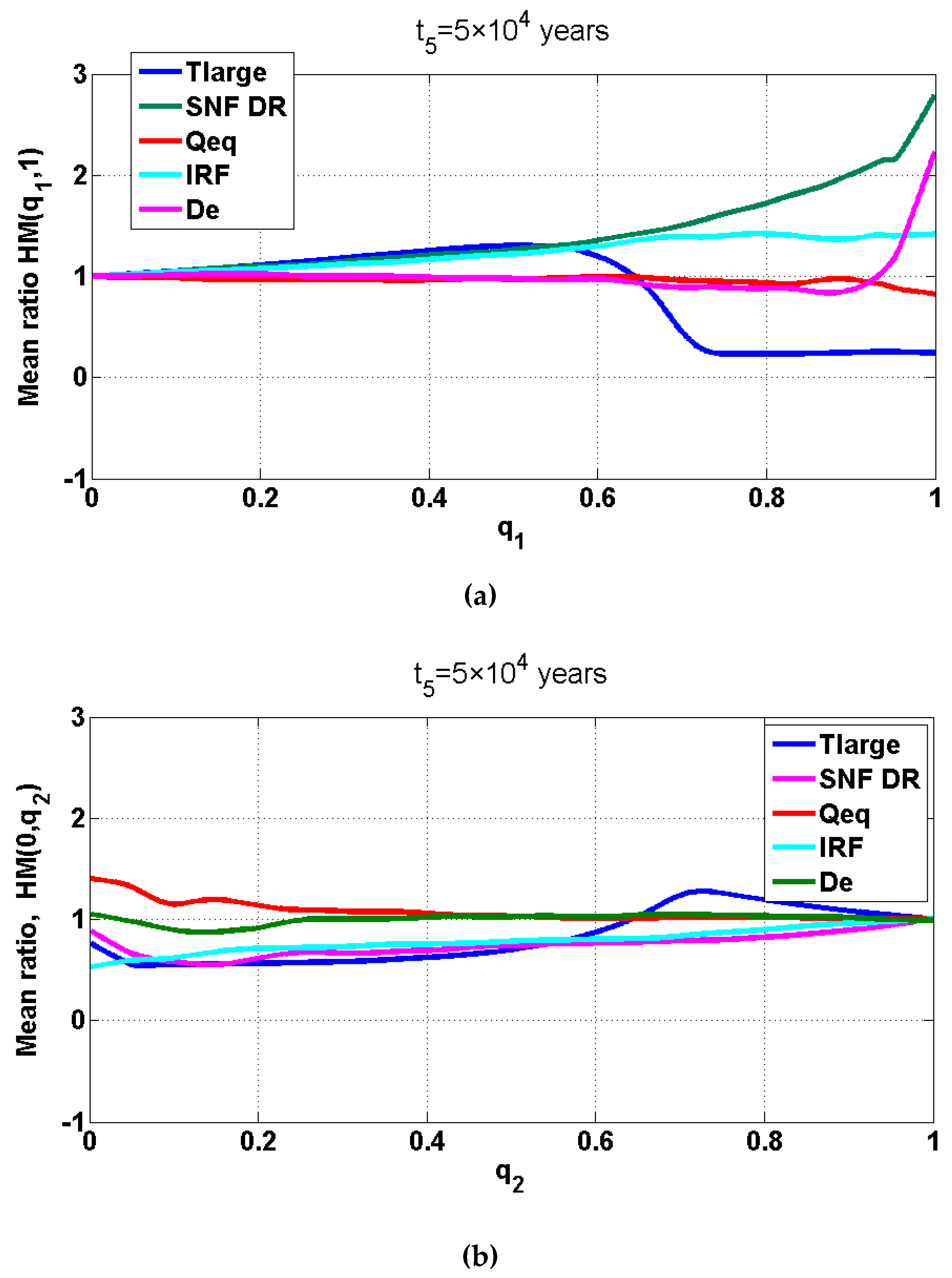
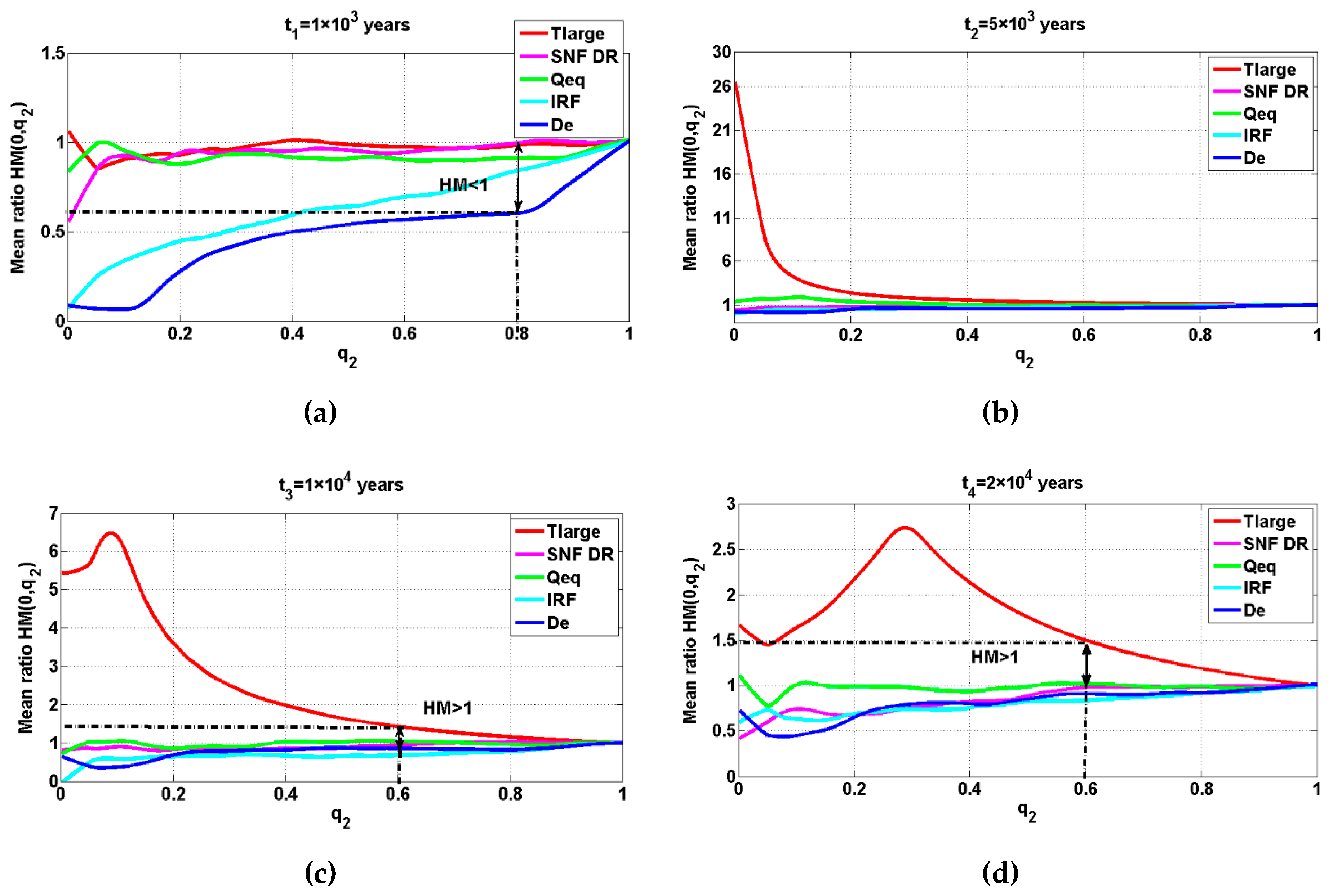
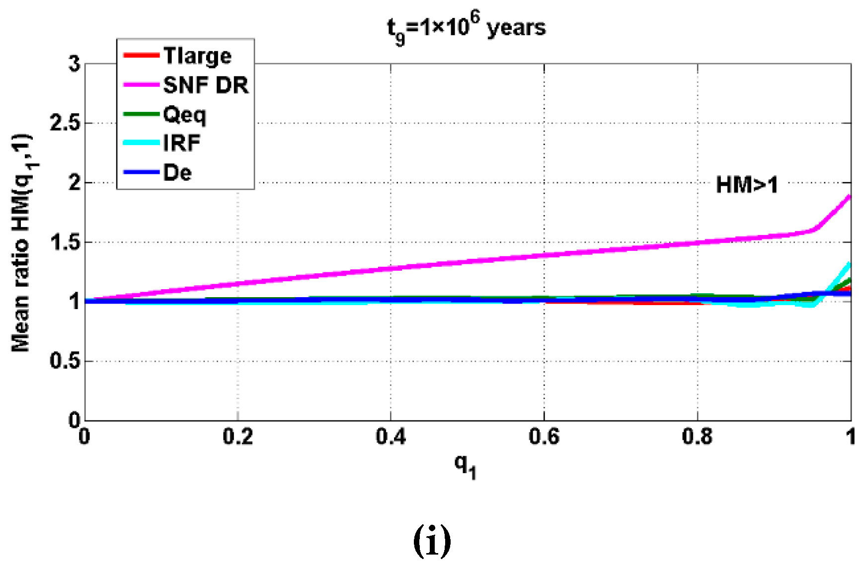
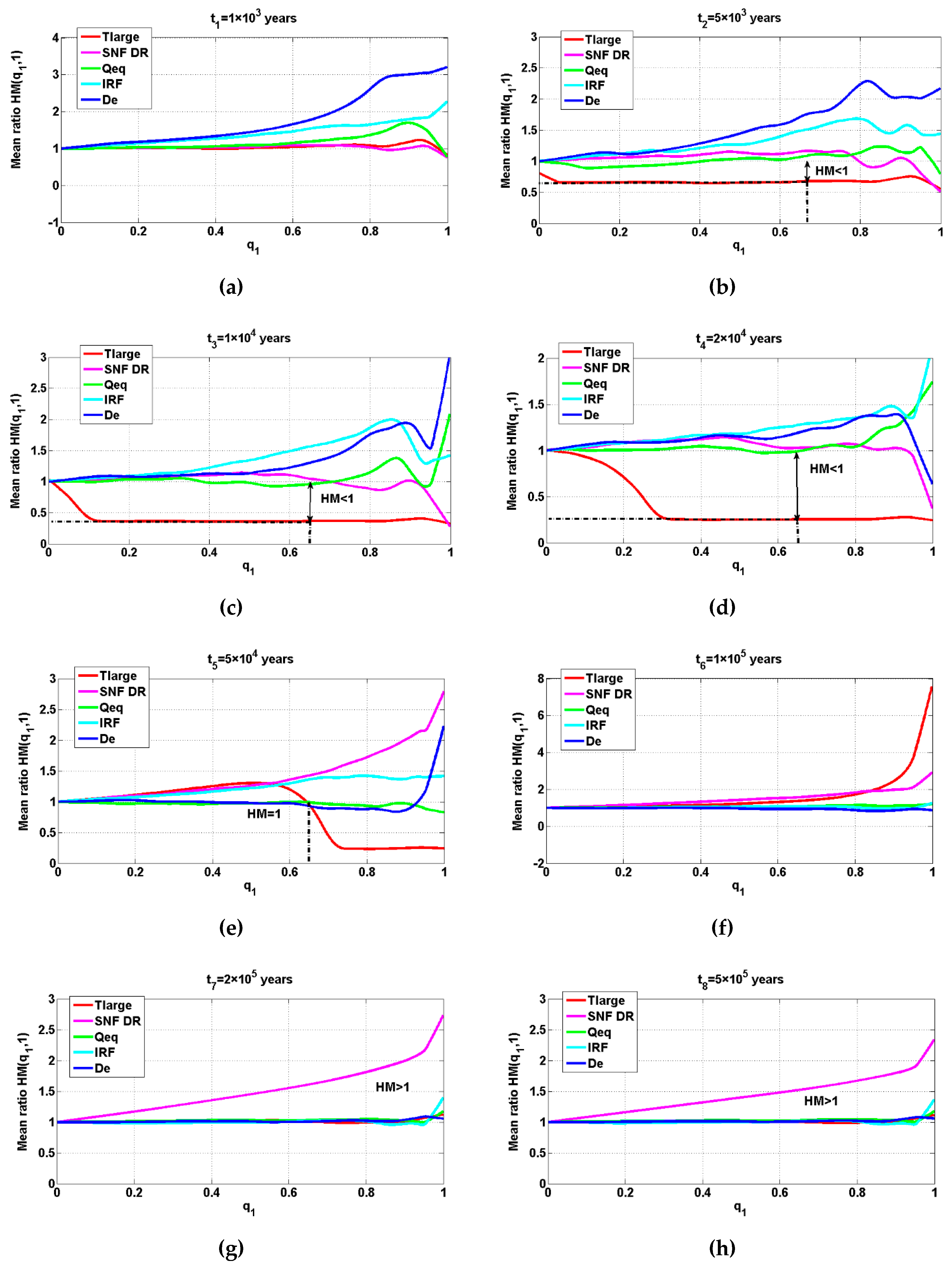
3.2.1. Mean Ratio Function

2D plots of the mean ratio function were derived considering the following aspects:

(a)

a plot of HM keeping the lower bounding value of input parameter $X_i^{}$ at q₁ = 0 and varying the upper bounding value (from q₂ = 0 to q₂ = 1);

(b)

a plot of HM keeping the upper bounding value of input parameter $X_i^{}$ fixed at q₂ = 1 and varying the lower bounding value (from q₁ = 0 to q₁ = 1).

Figure 9 presents the effect of uncertainty reduction of input parameter $X_i^{}$ (Tlarge, SNF DR, Qeq, IRF, De) by increasing the lower bound while the upper bound remains unchanged (q₁, q₂ = 1) (Figure 9a), and by decreasing of the upper bound while the lower bound remains unchanged (q₁ = 0, q₂) (Figure 9b).

The plots in Figure 9 indicated where an effort could be made to improve the model output at t₅ = 5 × 10⁴ years after the closure.

Revision and justification of new uncertainty range of parameter Tlarge and decreasing its uncertainty would have a variable effect on the mean flux. Decreasing the upper bounding value of Tlarge range to q₂ > 0.65 would lead to an increased mean flux; assigning the lower value (q₂ < 0.65) would yield a reduced mean flux at the time being analyzed (t₅ = 5 × 10⁴ years). The value of Tlarge at q₂ = 0.65 for the sorted series of randomly sampled values (size N = 1000) was equal to 4.5 × 10⁴ years. Similarly, increasing the lower bound up to value at q₁ = ~0.65 while keeping q₂ constant and at its original value would result in an increased mean flux (ratio HM > 1). However, an increase to greater values (q₁ > 0.65) would lead to a significant reduction of the mean flux (see Figure 9).

The parameters SNF DR and IRF led to the lower mean flux by decreasing the upper bound of their value range. Parameters Qeq and De had a small impact on mean flux at time t₅ = 5 × 10⁴ years after closure.

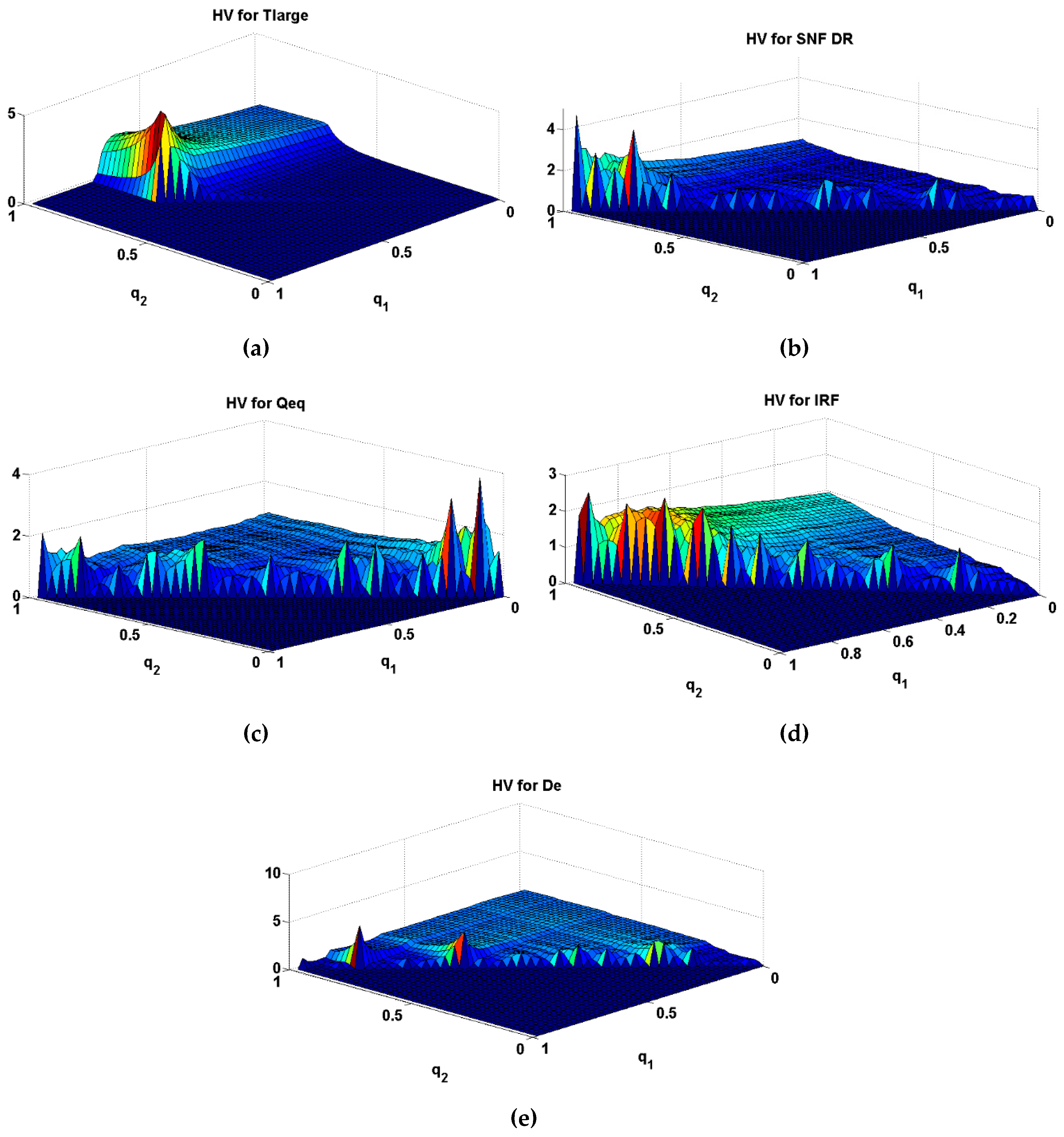
3.2.2. Variance Ratio Function

Similar to the effect on the mean flux, the effect of reducing the input parameter uncertainty on radionuclide flux (in terms of the variance) was estimated. Figure 10 presents the variance ratio functions due to:

(a)

reduced upper bound and

(b)

increased lower bound of the range of each parameter (at t₅ = 5 × 10⁴ years corresponding to the time of maximal mean flux).

As Figure 10 shows, increasing the lower bound of the input parameter Tlarge would result in increased radionuclide flux variance at the analyzed time (5 × 10⁴ years). This effect was similar to the estimated impact on the mean flux. Decreasing the upper bound of the parameter to value at q₂ = ~0.7 or less would result in the reduction of the flux variance only, while a reduction to value at q₂ > 0.7 would lead to slightly increased flux variance.

The impact of parameter SNF DR on the I-129 flux variance was similar to the effect on the mean. The increased lower bound of parameter range would lead to the higher flux variance, while the lower upper bound would affect decreased flux variance by a factor of ~2.

Justified uncertainty reduction by increasing the lower bound of parameter Qeq had some potential to result in decreased variance, which would be lower in comparison to some parameters, such as Tlarge, SNF DR, and IRF. For IRF, only a lower value of the upper bound would lead to a significant decrease in the flux variance. The effect of uncertainty reduction of parameter De would decrease the flux variance by up to 2 times only if the parameter uncertainty range is reduced significantly (to q₂ < 0.2).

3.3. Effect of Parameter Uncertainty Reduction on Mean Flux over Time

The time of the maximal mean flux could change with reduced parameter uncertainty. Thus, by fixing the parameter bound at certain quantile, the possible effect on the mean flux should be explored over the other time points.

For example, while fixing the upper bound of Tlarge at q₂ = 0.6 would cause the mean flux at time point t₅ to be reduced, the mean flux would be higher at earlier time points (t₃, t₄) by a factor of ~1.5 (see Figure 11c,d).

As Figure 11 demonstrates, reduced mean radionuclide flux could be observed in case of decreased upper bound of parameters SNF DR (ratio HM is less than 1) especially at a longer time scale (after 1 × 10⁵ years after closure). The figure also showed that for parameter SNF DR, decreasing the upper bound to the parameter value at, for example, q₂ = 0.8 (for the current sorted set of sampled values (N = 1000) it corresponded to 5.7 × 10⁻⁷ 1/year) would lead to a decrease in the mean flux by at least a factor of 1.14.

Reducing of the upper bound of IRF (at earlier times t₁–t₅) and D_e (soon after the start of radionuclide release) would also affect decreased mean flux as the HM ratio was less than 1.

On the other hand, increasing the lower bound of parameters SNF DR and IRF would lead to the increased mean as the ratio HM > 1 (see Figure 12).

Meanwhile, increasing the lower bound of parameter Tlarge to q₁ = 0.65 would result in a lower mean flux at time points t₂, t₃, t₄ and almost no change at time point t₅ (Figure 11). If such reduction cannot be justified, then changing q₁ to less than 0.65 would be expected to result in a lower mean at earlier times, but this would lead to an increased mean to some extent at time t₅. For the current set of sampled values (N = 1000), q₁ = 0.65 for parameter Tlarge corresponded to 4.6 × 10⁴ years.

As previously mentioned, increasing the lower bound of parameters SNF DR and IRF would lead to an effect on the increased mean as the ratio HM > 1 (Figure 12).

3.4. Summary of Discussion

It is clear that for the time-dependent variable of interest (model output), the manner of reducing input parameter uncertainty should only be done after an analysis of HM (HV) ratio evolution over time.

As presented, the performed analysis showed that the parameter ranking for I-129 time-dependent flux differed for different time points after repository closure. In the majority of cases, the ranking based on CSM and CSV methods was the same: soon after radionuclide release, the most significant parameter to contribute to mean flux and variance was the effective diffusivity of I-129 in bentonite (De); later, the defect size enlargement time (Tlarge) became dominant (up to 10⁵ years after the closure). At t = 1 × 10⁵ years after closure, the most significant contribution to the mean flux came from SNF dissolution rate (SNF DR), and the most significant contributor to the flux variance came from Tlarge. For longer periods (up to 1 million years after closure), the SNF DR was the main contributor to the mean flux and its variance.

The smallest and the largest values of SNF DR were the most significant contributors to the flux variance, which was not observed from the CSM plot.

Importance De (soon after the start of release) and SNF DR (in a long-term perspective) correlated with the regression analysis results; however, the greater importance of the defect size enlargement time was observed for the earlier time points (before 1 × 10⁵ years after the closure).

The analysis also showed that the effect of parameter uncertainty range reduction on the mean flux and its variance could be quantified without additional model runs by using the mean and variance ratio functions.

This study focused on the analysis of I-129 migration through engineered barriers. The observations were nuclide specific, and also depended on repository evolution conditions; therefore, in the case of other radionuclides or other disposal conditions, the analysis and parameter ranking exercise should be performed.

As CSM and CSV plots can be developed using the same set of sampled parameter values and do not require any additional model runs that are already available from probabilistic analyses, these tools provide additional valuable information for further research and have the potential to be applied more widely in the context of radioactive waste disposal.

4. Conclusions

With uncertainty and sensitivity analysis at a low value of determination coefficient of regression analysis, additional conclusions on parameter importance ranking have been drawn in case of I-129 flux from EBS of a conceptual disposal facility for RBMK-1500 SNF:

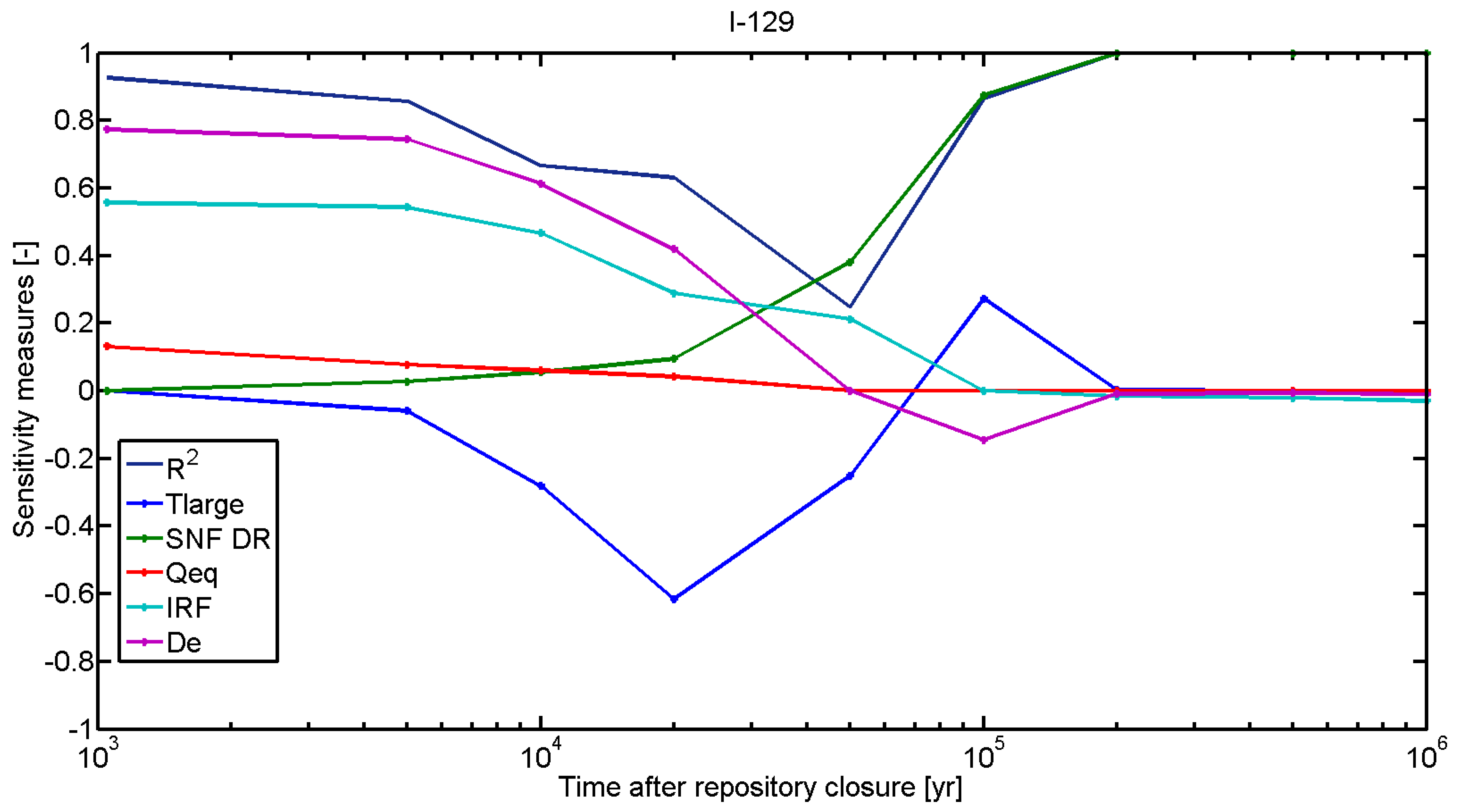
• The CSM identified defect size enlargement time on the I-129 time-dependent flux to have greater importance relative to the effective diffusivity in bentonite and instant release fraction of I-129 (identified in regression analysis) at earlier time points (for a period of 5 × 10³–5 × 10⁴ years after the repository closure). This importance ranking overcame the results from the regression analysis.
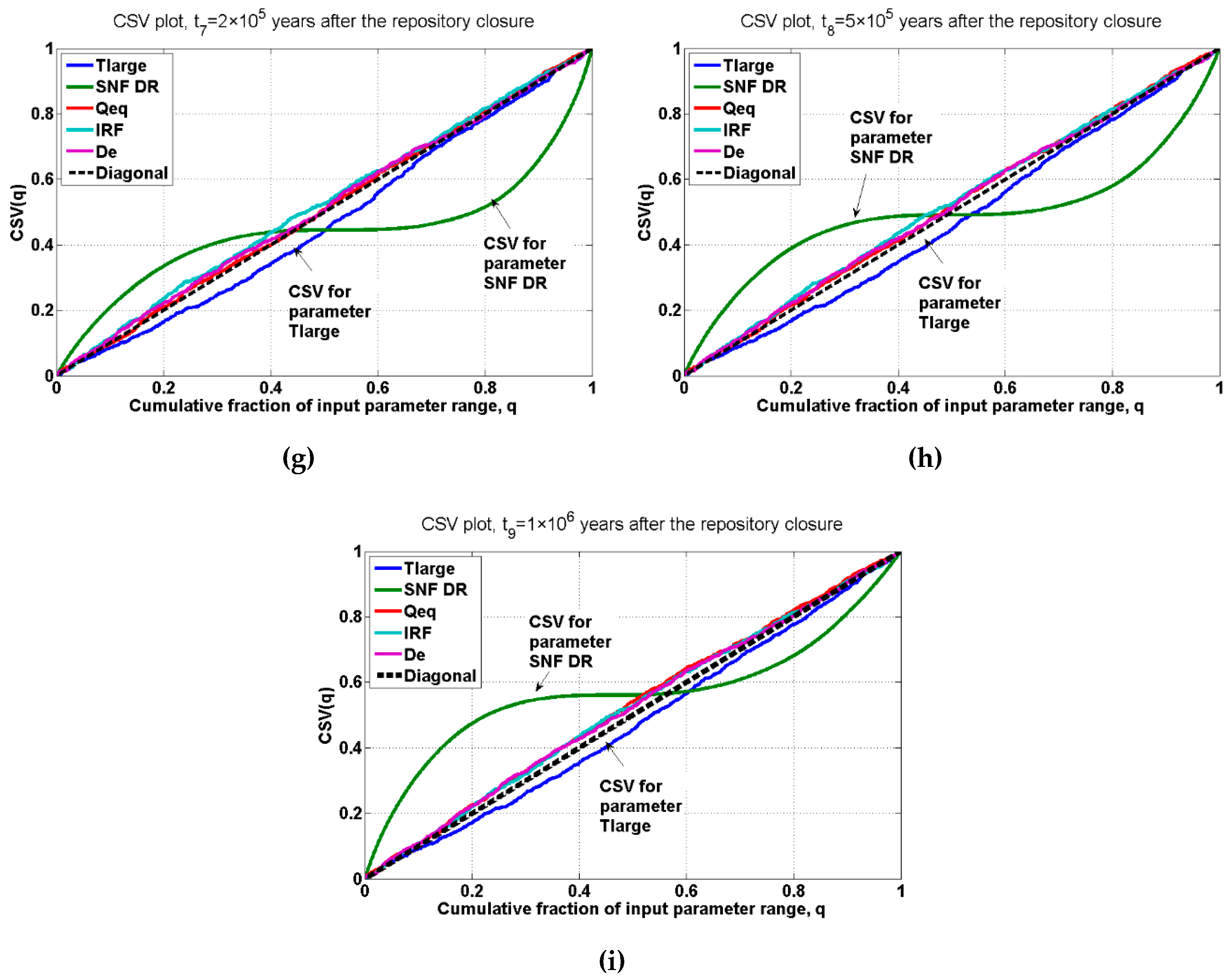
• The importance of defect size enlargement time was confirmed with the CSV method; its largest contribution to the variance of I-129 flux into the geosphere occurred at a time from 5 × 10³–10⁴ years after repository closure.
• Soon after the onset of radionuclide release, the most significant contributing parameter to the mean flux and its variance was effective diffusivity of I-129 in bentonite. For longer periods (up to 1 Million years after repository closure), the SNF dissolution rate was observed as the most significant contributor to the mean flux and its variance. These observations were in line with the results of the regression analysis.
• At t = 5 × 10⁴ years after repository closure (time of maximal mean flux), the most significant contributor to the mean flux was the SNF dissolution rate; however, the most significant contributor to flux variance was the defect size enlargement time.
• The effect of decreased mean flux before t = 5 × 10⁴ years after repository closure was observed from reduced defect size enlargement time uncertainty: if the lowest bounding value of the defect size enlargement time is increased to be 4.6 × 10⁴ years (parameter value at q₁ = 0.65), then the mean flux at t = 5 × 10³–2 × 10⁴ years would be lower. Almost no effect on the mean flux would occur at t = 5 × 10⁴ years after repository closure. If such input parameter range is not justified, then the increase to q₁ < 0.65 would lead to a lower mean at earlier time points and an increased mean (to some extent) at t = 5 × 10⁴ years after repository closure.
• If justification of the upper bounding value of the defect size enlargement time would lead to a value less than 4.6 × 10⁴ years (parameter value at q₂ less than 0.65), this would result in a decreased mean flux at t = 5 × 10⁴ years after the repository closure would be expected; however, this would cause increase in the mean flux at earlier time points. Fixing the upper bounding value of Tlarge to a value at q₂ = 0.6 would lead to the lower mean flux at t = 5 × 10⁴ years, but at earlier time t = 1 × 10⁴ years, t = 2 × 10⁴ years, the mean of flux would be greater by a factor of ~ 1.5.
• The effect of decreased mean flux in the long-term (up to 1 million years after closure) was observed in case of a justified reduction of the upper bound of the SNF dissolution rate only. Reducing parameter SNF DR uncertainty range from [10⁻⁸, 10⁻⁶] 1/year to [10⁻⁸, 5.7 × 10⁻⁷] 1/year (q₂ = 0.8) would lead to a decrease of mean flux by at least a factor of 1.14.
• CSM, CSV plots, and derived mean (variance) ratios have the potential to be applied more widely in the context of radioactive waste disposal as a means of complementing regression-based sensitivity analyses.

References

1. EC Directive 2011/70/Euratom. Available online: https://eur-lex.europa.eu/legal-content/EN/TXT/?uri=celex%3A32011L0070 (accessed on 20 March 2019).
2. Mellado, M.; Cisternas, L.A.; Lucay, F.A.; Gálvez, E.D.; Sepúlveda, F.D. A Posteriori Analysis of Analytical Models for Heap Leaching Using Uncertainty and Global Sensitivity Analyses. Minerals 2018, 8, 44. [Google Scholar] [CrossRef]
3. Frey, H.C.; Patil, S.R. Identification and Review of Sensitivity Analysis Methods. Risk Anal. 2002, 22, 553–578. [Google Scholar] [CrossRef] [PubMed]
4. Saltelli, A.; Annoni, P. How to avoid a perfunctory sensitivity analysis. Environ. Model. Softw. 2010, 25, 1508–1517. [Google Scholar] [CrossRef]
5. Cadinia, F.; De Sanctis, J.; Cherubini, A.; Zio, E.; Rivac, E.; Guadagnini, A. Nominal range sensitivity analysis of peak radionuclide concentrations in randomly heterogeneous aquifers. Ann. Nucl. Energy 2012, 47, 166–172. [Google Scholar] [CrossRef]
6. Pohjola, J.; Turunen, J.; Lipping, T.; Ikonen, A. Probabilistic assessment of the influence of lake properties in longterm radiation doses to humans. J. Environ. Radioact. 2016, 164, 258–267. [Google Scholar] [CrossRef]
7. Sinclair, J. Response to the PSACOIN Level S Exercise. PSACOIN Level S Intercomparison; Nuclear Energy Agency OECD: Paris, France, 1993. [Google Scholar]
8. Albrecht, A.; Miquel, S. Extension of sensitivity and uncertainty analysis for long term dose assessment of high level nuclear waste disposal sites to uncertainties in the human behaviour. J. Environ. Radioact. 2010, 101, 55–67. [Google Scholar] [CrossRef] [PubMed]
9. Aguero, A. Performance assessment model development and parameter acquisition for analysis of the transport of natural radionuclides in a Mediterranean watershed. Sci. Total Environ. 2005, 348, 32–50. [Google Scholar] [CrossRef]
10. Aguero, A.; Pined, P.; Cancio, D.; Simon, I.; Moraleda, M.; Perez-Sanchez, D.; Trueba, C. Spanish methodological approach for biosphere assessment of radioactive waste disposal. Sci. Total Environ. 2007, 384, 36–47. [Google Scholar] [CrossRef]
11. Aguero, A.; Pinedo, P.; Simón, I.; Cancio, D.; Moraleda, M.; Trueba, C.; Pérez-Sánchez, D. Application of the Spanish methodological approach for biosphere assessment to a generic high-level waste disposal site. Sci. Total Environ. 2008, 403, 34–58. [Google Scholar] [CrossRef]
12. Helton, J.C. Uncertainty and sensitivity analysis techniques for use in performance assessment for radioactive waste disposal. Reliab. Engng. Syst. Saf. 1993, 42, 327–367. [Google Scholar] [CrossRef]
13. Helton, J.C.; Davis, F.J.; Johnson, J.D. A comparison of uncertainty and sensitivity analysis results obtained with random and Latin hypercube sampling. Reliab. Engng. Syst. Saf. 2005, 89, 305–330. [Google Scholar] [CrossRef]
14. Bolado-Lavin, R.; Castaings, W.; Tarantola, S. Contribution to the sample mean plot for graphical and numerical sensitivity analysis. Reliab. Engng. Syst. Saf. 2009, 94, 1041–1049. [Google Scholar] [CrossRef]
15. Tarantola, S.; Kopustinskas, V.; Bolado-Lavin, R.; Kaliatka, A.; Uspuras, E.; Vaisnoras, M. Sensitivity analysis using contribution to sample variance plot: Application to a water hammer model. Reliab. Engng. Syst. Saf. 2012, 99, 62–73. [Google Scholar] [CrossRef]
16. Spiessl, S.M.; Becker, D.A.; Rubel, A. EFAST analysis applied to a Pa model for a generic HLW repository in clay. Reliab. Engng. Syst. Saf. 2012, 107, 190–204. [Google Scholar] [CrossRef]
17. Poskas, P.; Brazauskaite, A. Modeling of radionuclide releases from the geological repository for RBMK-1500 spent nuclear fuel in crystalline rocks in Lithuania. In Proceedings of the 11th International Conference ICEM2007, Bruges, Belgium, 2–6 September 2007. [Google Scholar]
18. Poskas, P.; Narkuniene, A.; Grigaliuniene, D.; Kilda, R. Analysis of radionuclide release through EBS of conceptual repository for Lithuanian RBMK spent nuclear fuel disposal—Case of canister with initial defect. Nukleonika 2013, 58, 487–495. [Google Scholar]
19. Poskas, P.; Narkuniene, A.; Grigaliuniene, D.; Finsterle, S. Comparison of radionuclide releases from a conceptual geological repository for RBMK-1500 and BWR spent nuclear fuel. Nucl. Technol. 2014, 185, 322–335. [Google Scholar] [CrossRef]
20. IAEA Tecdoc No. 1372. Safety Indicators for the Safety Assessment of Radioactive Waste Disposal; IAEA: Vienna, Austria, 2003. [Google Scholar]
21. Narkuniene, A.; Poskas, P.; Kilda, R.; Bartkus, G. Uncertainty and sensitivity analysis of radionuclide migration through the engineered barriers of deep geological repository: Case of RBMK-1500SNF. Reliab. Engng. Syst. Saf. 2015, 136, 8–16. [Google Scholar] [CrossRef]
22. Romero, L.; Moreno, L.; Neretnieks, I. Sensitivity of the radionuclide release from a repository to the variability of materials and other properties. Nucl. Technol. 1996, 113, 316–326. [Google Scholar] [CrossRef]
23. Shahkarami, P.; Liu, L.; Moreno, L.; Neretnieks, I. Radionuclide migration through fractured rock for arbitrary-length decay chain: Analytical solution and global sensitivity analysis. J. Hydrol. 2015, 520, 448–460. [Google Scholar] [CrossRef]
24. Hedin, A. Probabilistic dose calculations and sensitivity analyses using analytic models. Reliab. Engng. Syst. Saf. 2003, 79, 195–204. [Google Scholar] [CrossRef]
25. Stockman, C.T.; Garner, J.W.; Helton, J.C.; Johnson, J.D.; Shinta, A.; Smith, L.N. Radionuclide transport in the vicinity of the repository and associated complementary cumulative distribution functions in the 1996 performance assessment for the Waste Isolation Pilot Plant. Reliab. Engng. Syst. Saf. 2000, 69, 369–396. [Google Scholar] [CrossRef] [Green Version]
26. Helton, J.C.; Hansen, C.W.; Sallaberry, C.J. Uncertainty and sensitivity analysis in performance assessment for the proposed high-level radioactive waste repository at Yucca Mountain. Nevada. Reliab. Engng. Syst. Saf. 2012, 107, 44–63. [Google Scholar] [CrossRef]
27. Helton, J.C.; Johnson, J.D.; Sallaberry, C.J.; Storlie, C.B. Survey of sampling-based methods for uncertainty and sensitivity analysis. Reliab. Engng. Syst. Saf. 2006, 91, 1175–1209. [Google Scholar] [CrossRef] [Green Version]
28. Ragoussi, M.E.; Costa, D. Fundamentals of the NEA Thermochemical Database and its influence over national nuclear programs on the performance assessment of deep geological repositories. J. Environ. Radioact. 2019, 196, 225–231. [Google Scholar] [CrossRef] [PubMed]
29. Malekifarsani, A.; Skachek, M.A. Effect of precipitation, sorption and stable of isotope on maximum release rates of radionuclides from engineered barrier system (EBS) in deep repository. J. Environ. Radioact. 2009, 100, 807–814. [Google Scholar] [CrossRef] [PubMed]
30. Long-Term Safety for KBS-3 Repositories at Forsmark and Laxemar—A First Evaluation. Main Report of the SR-Can Project; SKB Technical Report TR-06-09; Swedish Nuclear Fuel and Waste Management Co.: Stockholm, Sweden, 2006.
31. Werme, L.O.; Johnson, L.H.; Oversby, V.M.; King, F.; Spahiu, K.; Grambow, B.; Shoesmith, D.W. Spent Fuel Performance under Repository Conditions: A Model for Use in SR-Can; SKB Technical Report TR-04-19; Swedish Nuclear Fuel and Waste Management Co.: Stockholm, Sweden, 2004. [Google Scholar]
32. Nordman, H.; Vieno, T. Equivalent Flow Rates from Canister Interior into the Geosphere in a KBS-3H Type Repository; Working report 2004-06; Posiva Oy: Eurajoki, Finland, 2004. [Google Scholar]
33. Ochs, M.; Talerio, C. Data and Uncertainty Assessment. Migration Parameters for the Bentonite Buffer in the KBS-3 concept; SKB Technical Report TR-04-18; Swedish Nuclear Fuel and Waste Management Co.: Stockholm, Sweden, 2004. [Google Scholar]
34. Enviros Quanitsci. AMBER 4.4. Getting Started. Version 1.0/User’s Manual; Enviros Quanitsci: Oxfordshire, UK, 2002. [Google Scholar]
35. Manache, G.; Melching, C.S. Identification of reliable regression-and correlation-based sensitivity measures for importance ranking of water-quality model parameters. Environ. Model. Softw. 2008, 23, 549–562. [Google Scholar] [CrossRef]
36. Wei, P.; Lu, Z.; Ruan, W.; Song, J. Regional sensitivity analysis using revised mean and variance ratio functions. Reliab. Engng. Syst. Saf. 2014, 121, 121–135. [Google Scholar] [CrossRef]
Figure 1. Dimensions of the engineered barriers of repository [21].
Minerals 09 00521 g001
Figure 2. The flux of I-129 flux from the engineered barriers (results of the first 20 realizations and the mean flux) from [21].
Minerals 09 00521 g002
Figure 3. Standardized rank regression coefficients (SRRC) as parameter importance measures and the coefficient of determination R2 over the analyzed period for I-129 flux as presented in [21] (R2—coefficient of determination, Tlarge—defect size enlargement time, SNF DR—SNF (spent nuclear fuel) matrix dissolution rate, Qeq—equivalent groundwater flow rate around the canister, IRF—instant release fraction, De—effective diffusivity of I-129 in bentonite).
Minerals 09 00521 g003
Figure 4. The CSM (contribution to the sample mean) plots for I-129 radionuclide flux into the geosphere (random sample size N = 1000) at different time points after the repository closure: (a) at 1 × 10³ years after repository closure; (b) at 5 × 10³ years after repository closure; (c) at 1 × 10⁴ years after repository closure; (d) at 2 × 10⁴ years after repository closure; (e) at 5 × 10⁴ years after repository closure; (f) at 1 × 10⁵ years after repository closure; (g) at 2 × 10⁵ years after repository closure; (h) at 5 × 10⁵ years after repository closure; (i) at 1 × 10⁶ years after repository closure (Tlarge—defect size enlargement time, SNF DR—SNF matrix dissolution rate, Qeq—equivalent groundwater flow rate around the canister, IRF—instant release fraction, De—effective diffusivity of I-129 in bentonite).
Minerals 09 00521 g004aMinerals 09 00521 g004b
Figure 5. The CSV (contribution to sample variance) plots for I-129 radionuclide flux into the geosphere (random sample size N = 1000) at different time points after the repository closure: (a) at 1 × 10³ years after repository closure; (b) at 5 × 10³ years after repository closure; (c) at 1 × 10⁴ years after repository closure; (d) at 2 × 10⁴ years after repository closure; (e) at 5 × 10⁴ years after repository closure; (f) at 1 × 10⁵ years after repository closure; (g) at 2 × 10⁵ years after repository closure; (h) at 5 × 10⁵ years after repository closure; (i) at 1 × 10⁶ years after repository closure (Tlarge—defect size enlargement time, SNF DR—SNF matrix dissolution rate, Qeq—equivalent groundwater flow rate around the canister, IRF—instant release fraction, De—effective diffusivity of I-129 in bentonite).
Minerals 09 00521 g005aMinerals 09 00521 g005b
Figure 6. Scheme for the exploration of the effect of the uncertainty reduction on model output using ratios HM, HV for each parameter.
Minerals 09 00521 g006
Figure 7. 3D plots of the revised mean ratio function (HM) for all parameters at t5 = 5 × 10⁴ years: (a) defect size enlargement time (Tlarge); (b) SNF dissolution rate (SNF DR); (c) equivalent groundwater flow rate around the canister (Qeq) (m3/year); (d) instant release fraction (IRF) of I-129; (e) effective diffusivity of I-129 in bentonite(De) (m2/s).
Minerals 09 00521 g007
Figure 8. 3D plots of the revised variance ratio function (HV) for all parameters at t5 = 5 × 10⁴ years: (a) defect size enlargement time (Tlarge); (b) SNF dissolution rate (SNF DR); (c) equivalent groundwater flow rate around the canister (Qeq) (m3/year); (d) instant release fraction (IRF) of I-129; (e) effective diffusivity of I-129 in bentonite (De) (m2/s).
Minerals 09 00521 g008
Figure 9. The mean ratio functions (HM) due to (a) reduced upper bound and (b) increased lower bound of the range of parameters (Tlarge, SNF DR, Qeq, IRF, De) at t5 = 5 × 10⁴ years after repository closure (smoothed by the regression technique) (Tlarge—defect size enlargement time, SNF DR—SNF matrix dissolution rate, Qeq—equivalent groundwater flow rate around the canister, IRF—instant release fraction, De—effective diffusivity of I-129 in bentonite).
Minerals 09 00521 g009
Figure 10. The variance ratio functions (HV) due to (a) reduced upper bound and (b) increased lower bound of the range of parameters (Tlarge, SNF DR, Qeq, IRF, De) at t5 = 5 × 10⁴ years after repository closure (smoothed by the regression technique) (Tlarge—defect size enlargement time, SNF DR—SNF matrix dissolution rate, Qeq—equivalent groundwater flow rate around the canister, IRF—instant release fraction, De—effective diffusivity of I-129 in bentonite).
Minerals 09 00521 g010
Figure 11. Ratio of the mean (smoothed by the regression technique) due to the decreased upper bound of the range of parameters (Tlarge, SNF DR, Qeq, IRF, De) for different time points: (a) at 1 × 10³ years after repository closure; (b) at 5 × 10³ years after repository closure; (c) at 1 × 10⁴ years after repository closure; (d) at 2 × 10⁴ years after repository closure; (e) at 5 × 10⁴ years after repository closure; (f) at 1 × 10⁵ years after repository closure; (g) at 2 × 10⁵ years after repository closure; (h) at 5 × 10⁵ years after repository closure; (i) at 1 × 10⁶ years after repository closure (Tlarge—defect size enlargement time, SNF DR—SNF matrix dissolution rate, Qeq—equivalent groundwater flow rate around the canister, IRF—instant release fraction, De—effective diffusivity of I-129 in bentonite).
Minerals 09 00521 g011aMinerals 09 00521 g011b
Figure 12. Ratio of the mean (smoothed by the regression technique) due to the increased lower bound of the range of parameters (Tlarge, SNF DR, Qeq, IRF, De) for different time points: (a) at 1 × 10³ years after repository closure; (b) at 5 × 10³ years after repository closure; (c) at 1 × 10⁴ years after repository closure; (d) at 2 × 10⁴ years after repository closure; (e) at 5 × 10⁴ years after repository closure; (f) at 1 × 10⁵ years after repository closure; (g) at 2 × 10⁵ years after repository closure; (h) at 5 × 10⁵ years after repository closure; (i) at 1 × 10⁶ years after repository closure (Tlarge—defect size enlargement time, SNF DR—SNF matrix dissolution rate, Qeq—equivalent groundwater flow rate around the canister, IRF—instant release fraction, De—effective diffusivity of I-129 in bentonite).
Minerals 09 00521 g012aMinerals 09 00521 g012b