Applying Machine Learning and Automatic Speech Recognition for Intelligent Evaluation of Coal Failure Probability under Uniaxial Compression

Abstract

Acoustic emission (AE) monitoring is an effective tool to quantify the dynamic damage that may cause heavy casualties and huge property losses in rock engineering. Instead of traditional failure evaluation methods, in this paper, the coal failure mechanism is evaluated in a complicated geological environment under uniaxial compression tests by employing machine learning (ML) and automatic speech recognition (ASR). Taking advantage of the ASR technology, the Mel-frequency cepstrum coefficients (MFCC) were extracted as sample features, while ML was used to paradigm the artificial intelligent evaluation of the failure probability of coal (AIEFPC). Additionally, the five-fold cross-validation method was used to assess the AIEFPC predictive effect incorporating cumulative hits number, cumulative ring count, and amplitude as sample features. The influence of category weight on the prediction effect of AIEFPC on a different category of sample sets has been discussed and analyzed. The results show that AIEFPC has the potential to use the MFCC of the 40 ms AE segment at any time to predict the dangerous state of the coal sample with a prediction accuracy of >85%. The probability value of the hazardous samples is computed through AIEFPC that further helped in evaluating the reliability of the prediction results. It is inferred from the obtained results that a larger category weight value of the hazardous samples can improve the prediction accuracy of AIEFPC than the safe sample. This research provides a new way of effectively predicting the coal failure probability before the damage and failure that can be applied to worldwide case-studies.

1. Introduction

Coal and rock damage problems have been major concerns in various engineering fields, such as the extraction and storage of oil and gas resources, the excavation of large underground caverns, and the prediction of coal and rock dynamic disasters. Effectively predicting the coal and rock instability before the failure is highly desirable in engineering fields [1]. Acoustic emission (AE) monitoring technology is an effective method for the monitoring and early warning of dynamic coal and rock disasters [2]. Before the occurrence of such disasters, the total number of events, large energy events, signal spectrum, etc., will show a significant change in their patterns [3,4].

AE is an elastic wave generated by sudden release during the crack propagation of rock, which provides real-time characteristic information of the internal rock deformation [5,6]. Based on AE signal characteristics, the change of internal rock cracks can be predicted [7,8,9]. Zhang et al. [10] studied the thermal damage assessment of rocks and established a thermal damage evolution model considering both heating and cooling processes based on AE monitoring technology. Zhao et al. [11] studied the relationship between the load stress and the peak stress corresponding to the minimum average frequency centroid of the AE during the deformation and failure of the red sandstone specimen. Statistically, they analyzed the distribution characteristics of the AE in different frequency bands. Events [12], energy [13], amplitude [14,15], and counts [16] are commonly used traditional AE characteristic parameters. Large energy signals are generally released during the coal and rock mass failure state, significantly altering the AE parameters [17]. Li [18] studied the AE characteristics of four different rock uniaxial compression failure and on-site rock mass failure processes. They concluded that the AE signal of low-stress-level rock is quite rare. AE activities increase when the stress reaches more than 80% of the peak strength. Based on acoustic emission signal strength, the rock mass failure process is divided into four stages: initial, severe, descending, and silent. Ganne [19], Liu [8], Jiang [20], and the references therein have also obtained the same conclusions. Many research results have been obtained by using the traditional AE feature parameters to analyze the coal rock failure process. They promote the application of AE monitoring technology in coal and rock dynamic disaster monitoring and early warning, and make great contributions to coal mines’ safe production. AE and coal damage have strong nonlinear characteristics. It is difficult to quantitatively analyze the damage and failure of coal using traditional AE characteristic parameters.

In the field of automatic speech recognition (ASR), the Mel-frequency cepstrum coefficient (MFCC) is the coefficient of the Mel-scale nonlinear transformation that composes the logarithmic energy spectrum. MFCC has always been the most widely used sound signal feature extraction technology [21] and is also commonly used in waveform recognition technical fields [22,23]. AE and sound signals are essentially the same: both are mechanical waves, but may exhibit different characteristics. Therefore, the ASR feature extraction technology is theoretically applicable to the analysis of the AE characteristics of coal and rock. Wang et al. [24] defined the ratio of coal sample stress to strength as the stress state, and studied the change law of the MFCC of AE during the uniaxial compression failure process of 55 coal samples, and found that the MFCC of AE and the stress state of the coal satisfy a linear relationship. The MFCC can be used to evaluate the damage state of the coal sample. The MFCC of AE comprises high-dimensional data composed of several coefficient values. Hence, analyzing the high-dimensional MFCC of AE is comparatively complex compared to traditional analysis methods.

Machine learning (ML) can take historical data as a training set and use an optimization algorithm to establish a feature and label relationship model, which can analyze high-dimensional data. ML, such as logistic regression (LR), classification regression tree (CART), and support vector machine (SVM), have been applied to study AE and the microseismic signal characteristics of the coal and rock failure process [25]. The MFCC of AE and the stress state of the coal satisfy a linear relationship; therefore, LR has been chosen as a basis for the ML algorithm. LR is a generalized linear model that uses the logarithmic probability function as the connection function. It has the characteristics of simple form, fast training speed, and strong generalization ability [26]. Compared with the traditional statistical methods, LR is capable of solving at higher dimensions, possesses a faster training speed and has a more vital generalization ability to handle larger data volumes [17,22], and has been widely used in disaster prediction [27], slope stability evaluation, and coal and gas outburst prediction [28]. The MFCC of AE and the coal sample’s stress state satisfy a linear relationship [29]. Better constraints can be obtained on evaluating coal and rock damage state by comprehensively using the MFCC of the AE and the logistic regression model. Consequently, the purpose of this article is to construct an artificially intelligent evaluation of the failure probability of coal (AIEFPC) based on AE data by the coupled use of ML and ASR.

In order to realize the purpose of using AE data to evaluate the failure possibility of coal samples, the AE waveform data of the uniaxial compression failure of 10 coal samples were collected, of which eight coal samples were used as the training set, and another two coal samples were used as the test set. The AE data were divided into AE segments with a length of 40 ms, and each segment was taken as an AE sample for AIEFPC. We used the MFCC approach in the ASR methodology to extract the MFCC of AE as the sample features and set the AE sample label corresponding to the stress state of the coal sample. The AIEFPC was constructed using the LR of machine learning. A five-fold cross-validation method was used to evaluate the prediction effect of the AIEFPC model. The prediction effect of the AIEFPC was compared with the traditional AE parameters such as cumulative hits, cumulative ring count, and amplitude; it was also compared when different combinations of MFCC were used as sample features. The influence of the category weight of the sample on the prediction effect of the AIEFPC on various sample sets is discussed. The research results can be used to identify the precursory information of AE for coal failure and can effectively predict the coal failure probability before the occurrence of damage and failure. The work provides a new analysis method for the application of AE monitoring technology in coal and rock dynamic disaster monitoring and early warning.

2. Data and Methods

2.1. Dataset

To realize the purpose of using AE data for the evaluation of the failure possibility for the coal sample, AE waveform data during the uniaxial compression loading of 10 coal samples were collected, of which eight coal samples were used as the training set, and another two coal samples were used as the test set.

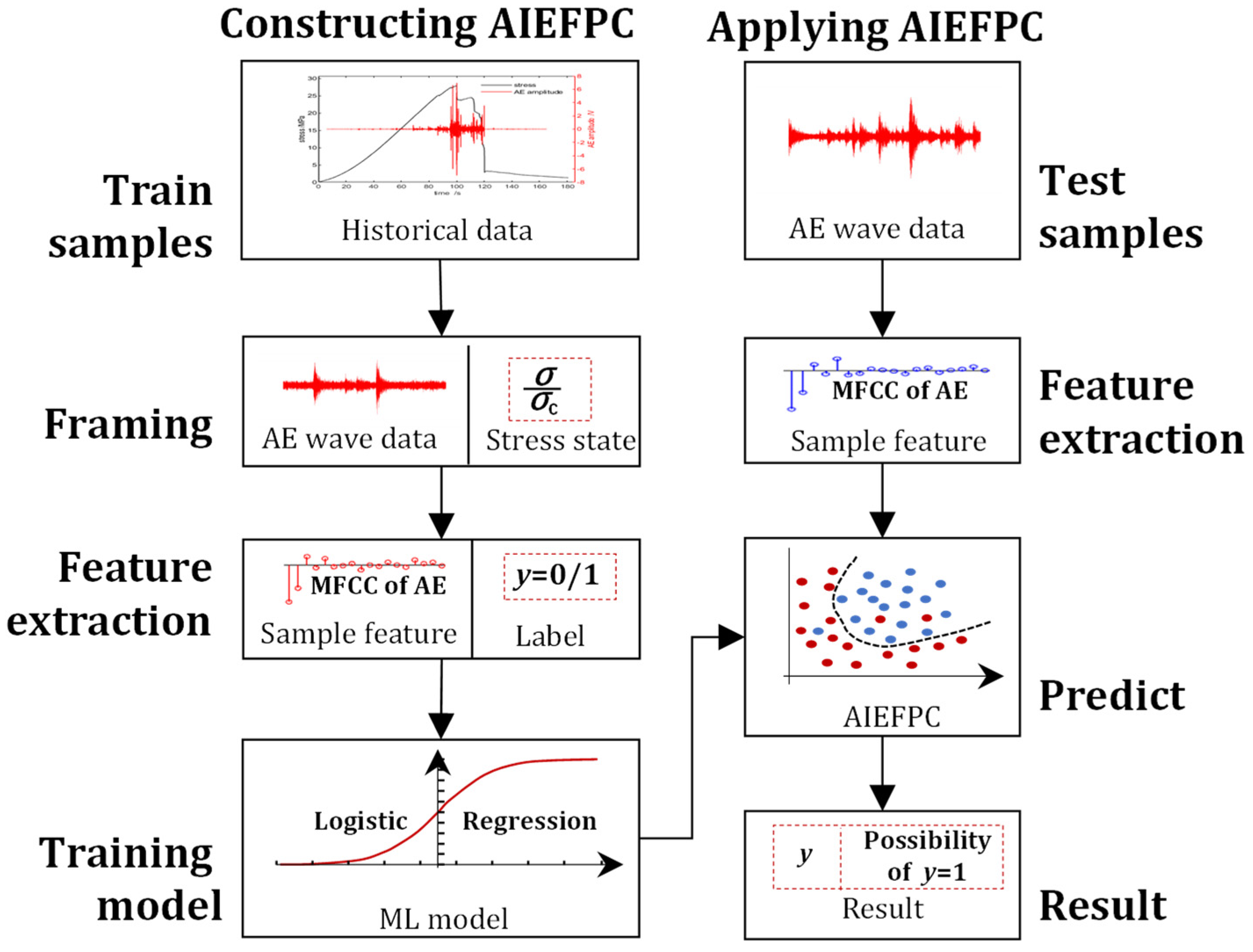
2.2. Generalized Procedure for AIEFPC Model

The stepwise procedure of creating and applying AIEFPC based on ASR and ML is presented in Figure 1, while the process of AE framing, AE sample feature extraction, and sample label production of AIEFPC is shown in Figure 2.

The specific required methodological procedure for the construction and application of AIEFPC is as follows.

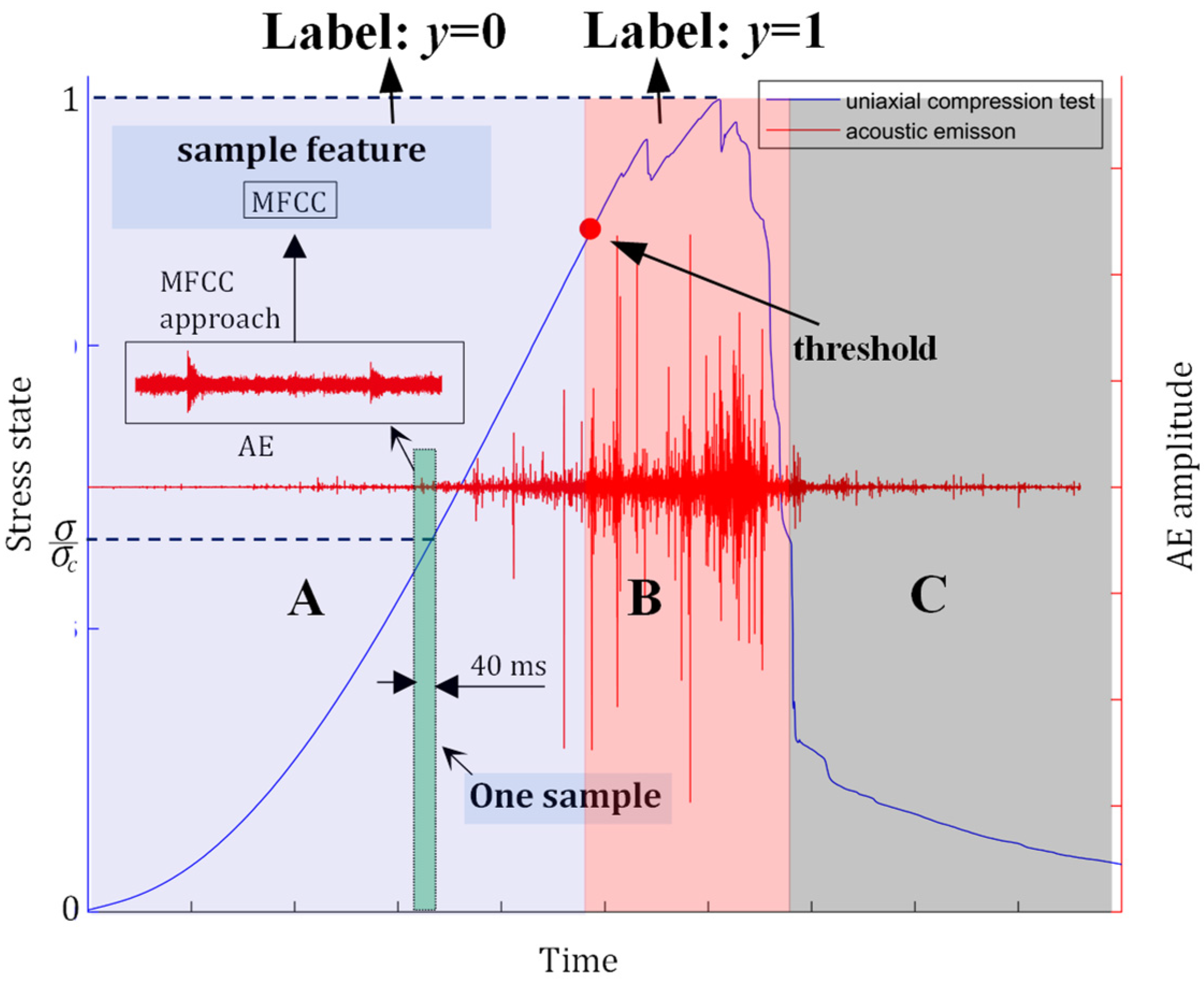
2.2.1. AE Sample Segmentation

The historical AE waveform data of the coal uniaxial compression loading process are set as the training set, and the AE data of the training set are divided into segments of equal length. One AE segment is taken as a sample. The experimental AE data collection and the uniaxial compression experiment are carried out synchronously, and the AE sampling rate is 1 MHz. The length of each frame of the AE signal is set to be 2 ms, which contains 2000 data points, i.e., the Window Length is 2000. The overlap of adjacent frames is set to be 0.5 ms, i.e., the Overlap Length is 500. Hence, the actual time interval between two adjacent frames is 1.5 ms. In other words, every 1.5 ms corresponds to a set of MFCC. In the experiment, the collection rate of the stress and strain data is 25 Hz, i.e., the time interval between adjacent stress and strain data points is 40 ms, and the 40 ms period contains 40,000 AE data points, corresponding to 26 sets of MFCC. So, we take an average of the 26 sets of MFCC in 40 ms to obtain a set of mean values of MFCC, which correspond to one stress data point. In this way, the MFCC and stress points are correlated one-to-one. The AE data segmentation is shown in Figure 3.

2.2.2. Sample Feature Extraction and Labeling

The feature extraction technology of sound features in ASR is employed to extract the MFCC of AE as the sample feature. The ratio of the coal sample’s stress state to its compressive strength is defined as the stress state of the coal sample. The dividing point is taken as the stress state exceeds the critical value for the first time. As shown in area A in Figure 2, the AE sample corresponding to the stress state less than the critical value is taken as the safe sample, and the sample label y = 0. As shown in area B in Figure 2, the AE sample corresponding to the stress state greater than or equal to the critical value is taken as a hazardous sample and the sample label y = 1.

The training artificial intelligence model uses an artificial intelligence algorithm to train and establish an artificial intelligence model describing the relationship between sample feature X and sample label y. The artificial intelligence algorithm used in this article is the LR. Based on the AE samples of the training set, the artificial intelligence model’s parameters are solved by the optimization algorithm, and the artificial intelligence model obtained is AIEFPC.

2.2.3. Applying AIEFPC

After calculating the estimated value of parameter θ of the AIEFPC, the extracted MFCC of AE is used as the sample feature X input into Equation (3) to calculate p(y = 1|X), the probability value of AIEFPC predicted sample label y = 1. When the p(y = 1|X) is less than 0.5, the AIEFPC output sample label is y = 0, and the AE sample is evaluated as a safe sample, the probability value is greater than or equal to 0.5, the AIEFPC output sample label y = 1, and the acoustic emission sample is evaluated as a hazardous sample. According to the probability value p(y = 1|X) of the output sample as the hazardous sample, the reliability of the model’s prediction results is judged.

2.3. Automatic Speech Recognition for AE Feature Extraction

As a useful feature, MFCC offers the advantages of a high success rate and a stable recognition effect. Since the AE and sound signals essentially exhibit the same characteristics and both are mechanical waves, the feature extraction technology in the ASR is theoretically applicable to the analysis of the AE characteristics of the coal and rock. MFCC is obtained by nonlinear transformation and has a strong correlation with the coal sample stress state [24]. The ASR’s MFCC approach is used as the AE feature extraction method, and the first 12 coefficients of the Mel-frequency cepstrum of the AE segments are taken as the sample feature X. The AE data collected during uniaxial compression loading of the coal samples is divided into equal length AE segments. Each AE segment is taken as an AE sample of the AIEFPC, as presented in Figure 4.

The scheme for the extraction of MFCC of the AE of coal is shown in Figure 4. The MFCC of the AE of coal involves three calculation steps. First, the AE data are divided according to the stationary characteristics of the AE signal to complete the framing of the AE data; then, the MFCC of each frame of the AE data are calculated, and finally, the average value of the MFCC is calculated as the key characteristic parameter of AE. Solving the MFCC of each AE data frame mainly includes five steps: windowing, fast Fourier transform (FFT), triangular window band-pass filter application, logarithm, and discrete cosine transform (DCT). A detailed description of AE feature extraction using MFCC can be found in reference [30].

2.4. Machine Learning for AIEFPC Model Training

The artificial intelligence algorithm for building AIEFPC selects a linear model with a simple form, fast training speed, and strong generalization ability. The generalized linear model expression is given in [31] as follows:

$$y=g^{-1}\left({\displaystyle \sum _{n=1}^N{w}_n{x}_n}+b\right)$$

(1)

where g (·) is the link function, w_n is the coefficient of the sample feature x_n of the linear model, b is the intercept of the linear model, and N is the number of sample features.

Binary classification is generally used for predicting whether the stress state of the coal is greater than the critical value, and to evaluate whether the coal sample will be a failure. The LR is a generalized linear model that uses the logarithmic probability function as the link function and is a binary classification model with excellent performance. The posterior probability estimation p(y = 1|[x₁, x₂,…, x_N, 1]) of the AE sample is the safe sample, and the posterior probability estimation p(y = 1|[x₁, x₂,…, x_N, 1]) of the AE sample is the safe sample, satisfying the following expressions, respectively [32]:

$$\ln \frac{p\left(y=1\left|\left[x_1,x_2,\cdots ,x_N,1\right]\right.\right)}{p\left(y=0\left|\left[x_1,x_2,\cdots ,x_N,1\right]\right.\right)}={\displaystyle \sum _{n=1}^N{w}_n{x}_n}+b$$

(2)

Order $\theta =[w_1,w_2,\cdots ,w_N,b],\hspace{1em}X=[x_1,x_2,\cdots ,x_N,1]$, take it into Equation (2), and we obtain:

$$p\left(y=1\left|X\right.\right)=\frac{e^{{\theta }^{T}X}}{1+e^{{\theta }^{T}X}}$$

(3)

$$p\left(y=0\left|X\right.\right)=\frac{1}{1+e^{{\theta }^{T}X}}$$

(4)

Use the maximum likelihood method to estimate the parameter θ value, for the training set {X_i, y_i} containing M samples, where y_i ∈ {0,1}, I = 1, 2, …, M, the likelihood of the logistic regression model function is [32]:

$${\displaystyle \prod _{i=1}^{M}p{\left(y=1|X_i\right)}^{y_i}}p{\left(y=0|X_i\right)}^{1-y_i}$$

(5)

The log-likelihood function is [32]:

$$L\left(\theta \right)={\displaystyle \sum _{i=1}^m\left(-y_i{\theta }^T{X}_i+\ln (1+e^{{\theta }^T{X}_i})\right)}$$

(6)

When L(θ) is the maximum value, the estimated value of parameter θ is obtained. The training process of AIEFPC is transformed into an optimization problem with log-likelihood as the objective function. The high-order derivable continuous convex function of θ is described in Equation (6). According to the convex optimization theory, numerical optimization algorithms such as the gradient descent method and the Newton method can be used to obtain the optimal solution. The limited-memory Broyden–Fletcher–Goldfarb–Shanno (L-BFGS) is the optimized algorithm used in this article, which belongs to quasi-Newton methods [33]. It approximates the Broyden–Fletcher–Goldfarb–Shanno (BFGS) algorithm using limited computer memory. It can often achieve a better solution than the two methods mentioned above with fewer iterations [34,35].

2.5. Parameter Setting

As described in Section 3, the uniaxial compression experiment uses two control methods, namely, axial stroke control and axial stress control, with five coal samples for each control method. The AE waveform data of a total of 10 coal samples during uniaxial compression failure are used in this paper. Among them, eight coal samples were used as the training set and two coal samples were used as the test set. The frequency of AE data acquisition is 1 MHz. A 40 ms AE segment is used as an AE sample of the AIEFPC; one AE sample contains 40,000 waveform data, and the first 12 coefficient values of the Mel-frequency cepstrum of the AE are used as the sample feature. A computer program for solving the MFCC of AE samples is developed based on MATLAB’s mfcc function. The parameters for solving MFCC are shown in reference [24]. Set the critical value of the stress state to 0.8, and the corresponding AE sample with the stress state less than 0.8 is set as a safe sample, marked as a positive sample, and the sample label y = 0; when the stress state is greater than or equal to 0.8, the corresponding AE sample is set as a hazardous sample, marked as a negative sample, sample label y = 1.

The training and use of AIEFPC are implemented through Python language programming, and the LR is implemented using the Logistic Regression class in scikit-learn 0.23.2 [33]. Setting the class weight parameter class_weight = {0:1,1:1} and the regularization parameter penalty = ‘none’ obtains a Logistic Regression object that does not use regularization and class weight balance. The fit method of the Logistic Regression object was used to train AIEFPC. Using the coef_ of the Logistic Regression object obtains the value of the AIEFPC parameter θ. The predict and predict_proba methods of the Logistic Regression object are used to obtain the sample label and the probability value of the sample as a hazardous sample. Other parameters of the AIEFPC construction, use, and testing process use the default parameters of scikit-learn 0.23.2.

2.6. Evaluation of Model Performance

To scrutinize and evaluate the hazardousness of the coal sample, AIEFPC has been constructed. It belongs to a machine learning model that solves binary classification. Accuracy (ACC), true positive rate (TPR), and true negative rate (TNR) are three commonly used indicators to evaluate the prediction performance of the binary classification [36]. In this paper, ACC is the prediction accuracy of all of the AE samples in the test set. The TPR is the prediction accuracy of the safe sample, and the TNR is the prediction accuracy of the hazardous sample. The ACC, TPR, and TNR are calculated based on the confusion matrix shown in

Table 1. Confusion matrix for a binary classification problem [37].

Actual Situation	Predicted Result
	Positive	Negative
Positive	TP	FN
Negative	FP	TN

Note: TP is true positive and means the number of positives predicted as positive; FN is false negative and indicates the number of positives predicted as negative classes; FP is false positive and represents the number of negatives predicted as positive, and TN is true negative and means the number of negatives predicted as negative classes.

. The ACC, TPR, and TNR were calculated as follows:

$$ACC=\frac{TP+TN}{TP+TN+FP+FN}$$

(7)

$$TPR=\frac{TP}{TP+FN}$$

(8)

$$TNR=\frac{TN}{TN+FP}$$

(9)

3. Experiment and Samples

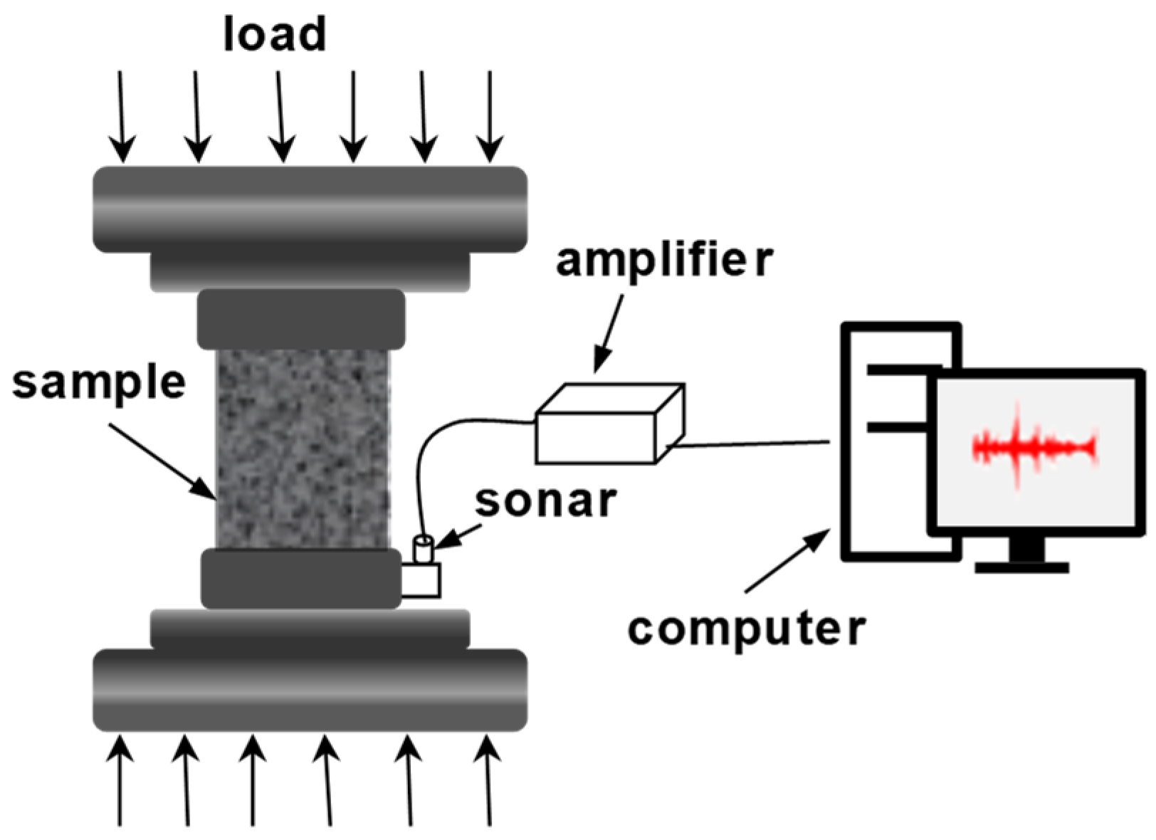
3.1. Experiment Facilities

The experimental loading system used the RMT-159 universal testing machine produced by the Wuhan Geotechnical Institute of the Chinese Academy of Sciences. The device offers multiple control methods such as axial stress control, axial stroke control, and axial strain control. To achieve the objectives of this study, we used axial stroke control and axial stress control in the experiment. For the loading rate of 0.010 mm/s, 0.5 kN/s, the stress and strain data collection frequency was set to 25 Hz.

The AE acquisition instrument adopts the DS2 AE acquisition system produced by Soft Island Company, Beijing, China, which enables the continuous real-time detection and acquisition of AE data. The AE sensor RS2-A was used at a frequency range of 50–400 kHz, a centre frequency of 150 kHz, and an amplifier gain of 20 dB. In this paper, the AE sensor was coated with petroleum jelly and attached to the test machine’s pressure head. The trigger mode of the AE acquisition instrument was set to manual trigger and the sampling frequency was set to 1 MHz. After the acquisition instrument had been triggered, the AE’s full-waveform data were saved until the end of the experiment. A schematic diagram of the experimental device is shown in Figure 5.

3.2. Specimen and AE Samples

The test coal samples were collected from the #8 coal seam of Dongqu Mine, of the Xi’shan Coal Sample Electricity Group, at Taiyuan, Shanxi province, China. The coal samples were processed into 50 mm × 50 mm × 100 mm square standard coal samples in the laboratory; then, 10 coal samples with few cracks and good integrity were divided into two groups for uniaxial compression testing with loading rates of 0.010 mm/s, 0.5 kN/s (see

Table 2. Coal sample numbering grouping.

Coal Mine	Sample	Length/mm	Width/mm	Height/mm	Strength/MPa	Load Rate
Dongqu mine	aD8-1	50.5	50.4	100.6	8.56	0.005 mm/s
	aD8-2	50.1	50.4	95.9	14.78	0.005 mm/s
	aD8-3	52.1	52.6	99.7	10.18	0.005 mm/s
	aD8-4	50.7	51	97.7	14.35	0.005 mm/s
	aD8-5	50.8	50.6	100.4	12.67	0.005 mm/s
	bD8-1	54.3	51.1	100.6	8.36	0.50 kN/s
	bD8-2	50.1	50.4	95.9	13.17	0.50 kN/s
	bD8-3	49.2	51.2	99.8	11.50	0.50 kN/s
	bD8-4	52.2	52	100.3	12.95	0.50 kN/s
	bD8-5	52.5	51.6	100.1	19.02	0.50 kN/s

).

The collected AE data were divided into 40 ms segments, and each AE segment was taken as an AE sample. The sample label is made based on the stress state of the coal. The AE samples with stress states less than 0.8 are marked as safe samples, and those with stress states greater than or equal to 0.8 are marked as hazardous samples. The statistics of the safe samples and hazardous samples in AE samples of each coal sample are shown in

Table 3. Statistics of the safe and hazardous samples in AE segments of each coal sample.

Coal Specimen	AE Segments			Coal Specimen	AE Segments
	Safe	Hazardous	Total		Safe	Hazardous	Total
aD8-1	3128	1122	4250	bD8-1	1510	440	1950
aD8-2	3029	889	3918	bD8-2	694	281	975
aD8-3	3526	874	4400	bD8-3	388	587	975
aD8-4	6681	1494	8175	bD8-4	1366	434	1800
aD8-5	5319	1675	3994	bD8-5	2306	593	2899

.

4. Results and Interpretation

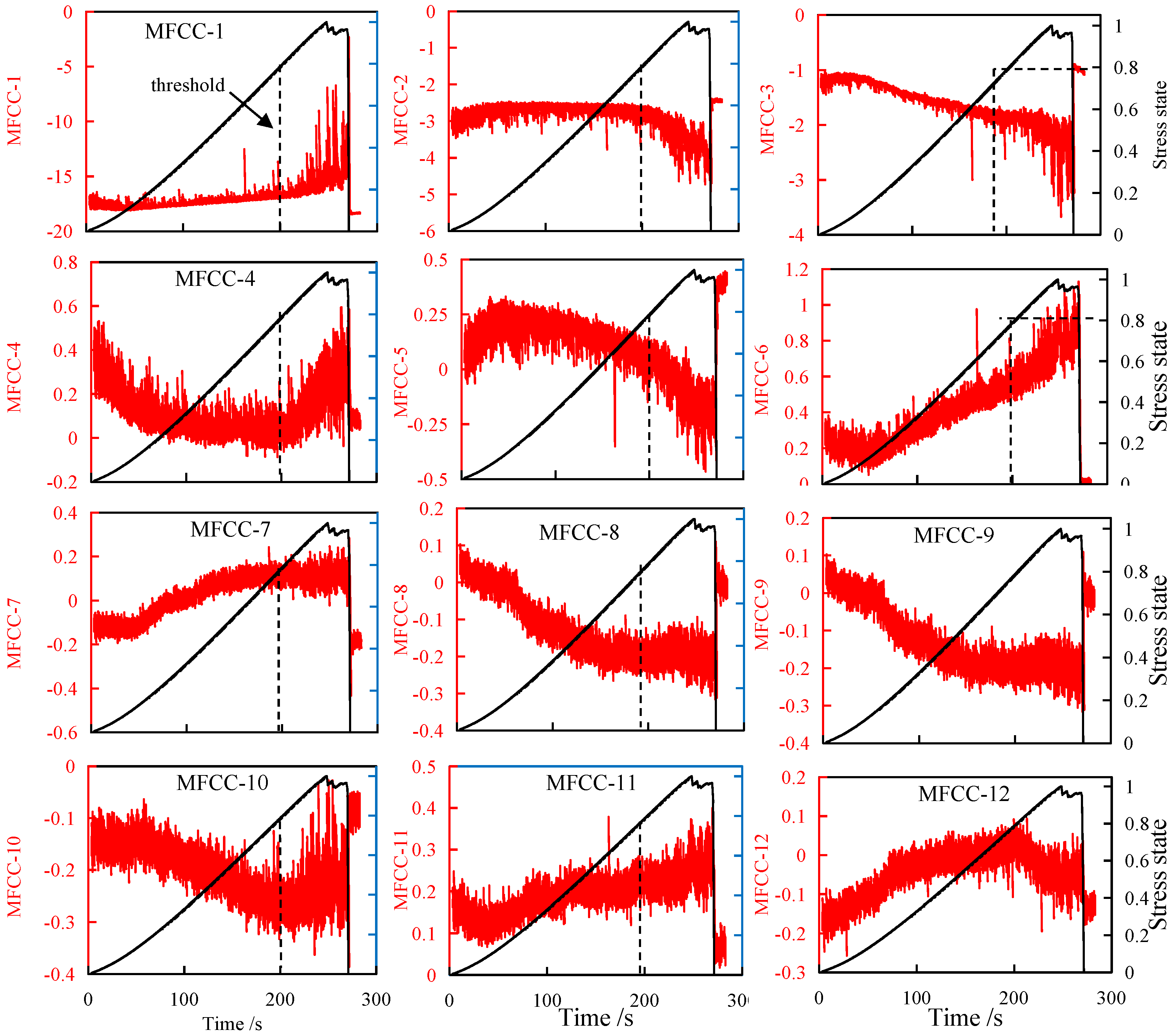
4.1. Correlation of Mel-Frequency Cepstrum Coefficients for Acoustic Emissions and Coal Specimen Stress State

As described in Section 2.5, the AE data were divided into segments of 40,000 data points in length. The corresponding values of the MFCC of AE under different stress states were calculated using MATLAB. Changes of the AE during the deformation and failure of coal with varying rates of loading remained the same. Limited by space, the coal sample of the #8 coal seam of Dongqu mine (numbered aD8-1) is used as an example to present the application effect of the MFCC approach on the AE signal’s features over the whole coal failure process. MFCC-n is used to represent the n-th parameter value of the Mel-frequency cepstrum of AE. Figure 6 shows the variation of the MFCC of AE and stress state with the time uniaxial compression experiment of the coal sample aD8-5.

MFCC-1, MFCC-2, MFCC-3, MFCC-5, MFCC-6, MFCC-7, MFCC-8, MFCC-9, MFCC-11, etc., are compared with the stress state strong correlation as shown in Figure 6. Through visual observation, it is evident that among these, MFCC-6 has the strongest correlation with the stress state. MFCC-1, MFCC-6, MFCC-7, and MFCC-11 increase with the increase in the coal sample stress state, and MFCC-6 increases linearly with the increase in the stress state. MFCC-2, MFCC-3, MFCC-5, MFCC-8, and MFCC-9 decrease with the increase in the coal sample stress state. When the stress state is less than 0.8, MFCC-2 generally remains unchanged, while MFCC-2 decreases rapidly when the stress state is greater than 0.8. MFCC-4, MFCC-10, and MFCC-12 have poor correlation with the stress state. Among them, MFCC-4 and MFCC-10 first decrease and then increase as the stress increases, and MFCC-12 first increases and then increases as the stress increases. The general characteristics of the change of MFCC with stress state can be obtained by visual observation. However, it is difficult to quantitatively describe the failure state of the coal samples using MFCC.

4.2. Prediction of Failure Probability of Coal Using AIEFPC

4.2.1. Characteristics of AIEFPC

In this paper, aD8-1, aD8-2, aD8-3, aD8-4, bD8-1, bD8-2, bD8-3, and bD8-4 have been taken as training coal samples, the AE waveform data in the process of coal failure are divided into 40 ms AE segments, and each AE segment is considered a training set sample. By taking the first 12 coefficient values of the extracted Mel cepstrum as the sample feature, MFCC-n is the n-th feature x_n in the sample feature X. Through the Logistic Regression class in scikit-learn 0.23.2, the Python language program is compiled, and the AIEFPC is trained by the AE samples of the training set. Using the coef_ attribute of Logistic Regression object extraction, the coefficient w_n corresponds to the feature MFCC-n in AIEFPC. The coefficient can be used to describe the characteristics of AIEFPC. Figure 7 is the absolute value of the coefficient w_n corresponding to the feature MFCC-n in AIEFPC. Blue indicates that w_n is a positive number, and red shows that w_n is a negative number.

MFCC-5, MFCC-6, MFCC-7, MFCC-8, MFCC-9, etc., present a good correlation with the stress state. As shown in Figure 7, these have relatively large coefficients in AIEFPC; however, MFCC-4 and MFCC-10, with a poor correlation with the stress state, are also larger. As described in Section 2.1, AIEFPC predicts the sample label based on the posterior estimated probability value p(y = 1|X) of the sample label y = 1. The logistic regression model is linear: the larger the product of θ^T*X, the greater the probability that the sample is hazardous. The larger the absolute value of the parameter w_n, the more sensitive the AIEFPC prediction result is to the change of the feature MFCC-n.

The coefficient w₈ corresponding to the MFCC-8 has the largest absolute value, and the coefficient w₁ corresponding to the MFCC-1 has the smallest absolute value. However, the contribution of the feature MFCC-8 to the AIEFPC prediction result is not as significantly important as the feature MFCC-1; when other parameters are unchanged, the larger the product x_n*w_n of the n-th feature x_n of the sample and the corresponding coefficient w_n, the larger the posterior estimated probability value p(y = 1|X) of the sample label y = 1. The probability value is simultaneously affected by the value of the sample feature x_n and the value of the sample feature corresponding coefficient w_n. It can be seen from Figure 6 that as the stress state increases, the value of MFCC-1 gradually increases from −17 to −5, the value of MFCC-8 decreases from 0.1 to −0.3, and the variation range of MFCC itself is inconsistent, so the absolute value of the sample feature coefficient w_n in AIEFPC does not truly reflect the importance of the sample feature. The significance of the sample feature will be analyzed in detail in Section 5.1.1.

4.2.2. Validation of Prediction Effect of AIEFPC

Five-fold cross-validation is a commonly used model evaluation method in verifying machine learning [31]. This paper uses the five-fold cross-validation method to evaluate the prediction effect of AIEFPC and verify the generalization ability of AIEFPC. Five-fold cross-validation is to divide the initial sampling set into five sub-samples. A single sub-sample is retained as the data for the verification model. The other four sub-samples are used for training [36]. This paper uses the uniaxial compression experiment results of 10 coal samples in the #8 coal seam of Dongqu Mine as the initial sample set. The coal samples of the train set and test set of the five-fold cross-validation are shown in Figure 8.

Through the Logistic Regression class in scikit-learn 0.23.2, the Python language program is compiled and the AIEFPC is trained by the AE samples of the training set. The AE waveform data of the test coal samples were divided into 40 ms AE segments. The first 12 coefficients of the Mel cepstrum extracted as sample feature X were input into AIEFPC to calculate the prediction results of the AE sample label. Compare the predicted AE sample label with the real label to obtain the confusion matrix of AIEFPC on the test set. The calculated ACC, TPR, and TNR results are shown in

Table 4. Confusion matrix, ACC, TPR, and TNR of five-fold cross-validation for evaluating AIEFPC performance.

Fold	TP	FN	FP	TN	ACC	TNR	TPR
Fold-1	3546	177	367	803	88.9%	68.6%	95.2%
Fold-2	3331	583	219	1248	85.2%	85.4%	85.1%
Fold-3	7060	987	471	1457	85.4%	75.6%	87.7%
Fold-4	4372	266	536	1026	87.1%	65.7%	94.3%
Fold-5	9671	654	135	2133	92.0%	94.0%	91.4%

.

The maximum prediction ACC of AIEFPC is 92.0%; the minimum value is 5.2%, as evident in Table 4. For predicting dangerous states of the coal sample, the AIEFPC displays strong generalization ability and can achieve satisfactory results. Using AIEFPC to evaluate the failure probability, the arbitrary continuous 40 ms AE waveform data in the process of coal rock uniaxial compression failure are used and the trend and historical data of the AE signal in the coal sample failure process are not used. AIEFPC can be used to predict the failure possibility of coal. The prediction accuracy is high, and the effect is stable, only based on more than 40 ms of AE data.

The maximum value of TPR is 95.2%, while the minimum value of TPR is 85.1%. AIEFPC has high accuracy and a stable effect in the safe sample set. The false alarm rate of the AIEFPC model in coal and rock dynamic disaster monitoring and early warning is low. However, the maximum value of TNR is 94% and the minimum value of TNR is 65.7%; thus, the accuracy of AIEFPC on the dangerous sample set is not ideal. In the application of dynamic disaster monitoring and early warning, the wrong classification of hazardous samples leads to a failure to raise the alarm, leading to serious consequences. Methods to improve the accuracy of AIEFPC in the hazardous set and reduce the occurrence of missing model alarms are analyzed in detail in Section 5.2.

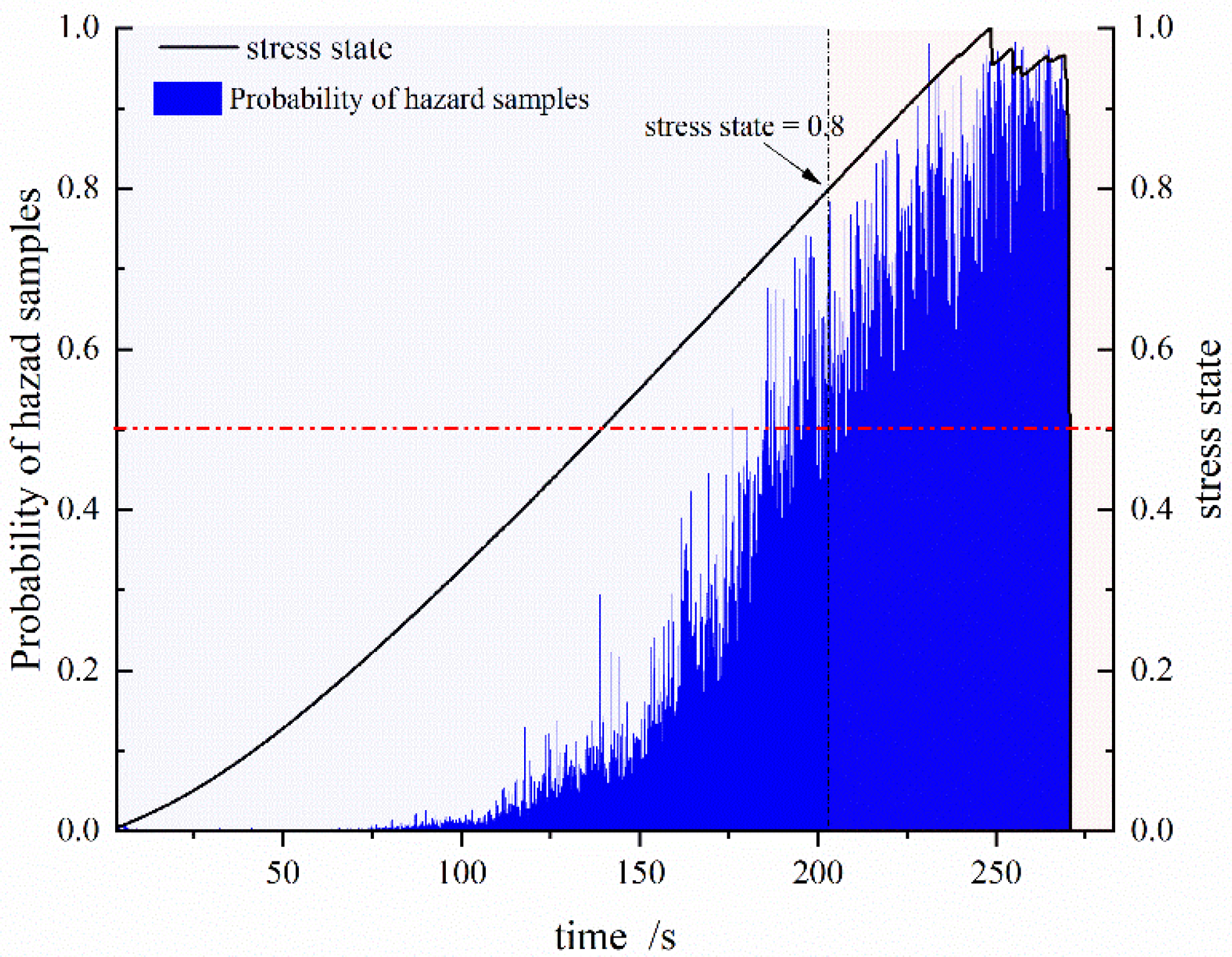
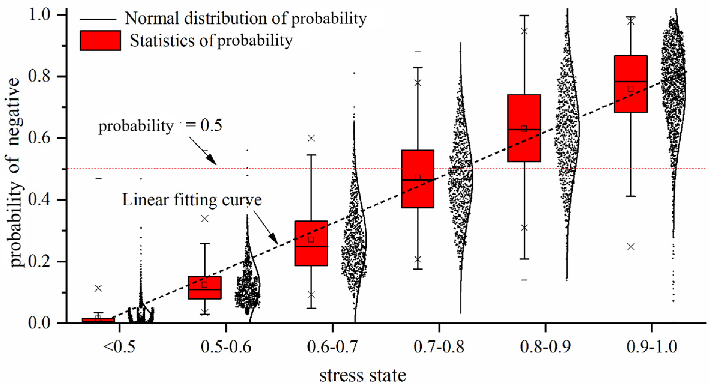
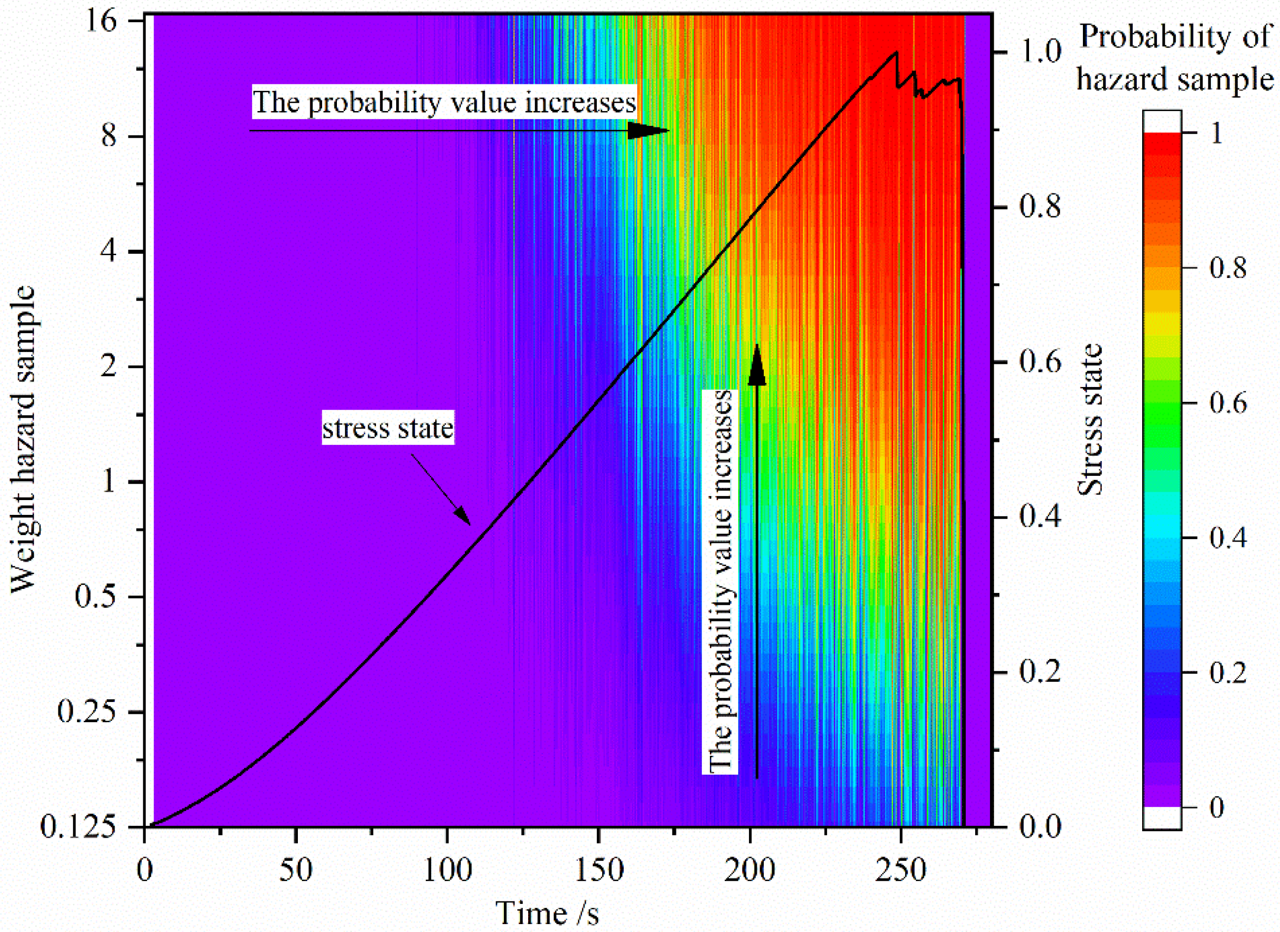
4.3. Probability of AE Samples Predicted as Dangerous Samples by AIEFPC

The training set and the test set are divided using Fold-5 in Figure 8. After the estimated value of the AIEFPC parameter θ is obtained by training, the MFCC of the AE fragment of an aD8-5 coal sample is taken as the sample feature X and entered into Equation (3) to calculate how AIEFPC predicts the probability that the AE sample is a hazardous sample. We use the predict_proba method of Logistic Regression class in scikit-learn 0.23.2 to calculate the AE sample’s probability value as a hazardous sample. Figure 9 shows the probability value that AIEFPC predicts the AE sample is a hazardous sample at the aD8-5 coal sample during uniaxial compression.

Figure 9 shows that as the stress state increases, the probability value that AIEFPC predicts that the AE sample is a hazard sample gradually increases, and the acoustic emission samples predicted as dangerous samples increase progressively. The larger the probability value, the closer the coal sample state is to the failure state. According to the stress state’s magnitude, the test set samples are divided into six categories of less than 0.5, 0.5–0.6, 0.6–0.7, 0.7–0.8, 0.8–0.9, and 0.9–1.0. The distribution of probability that AIEFPC predicts the hazardousness of the AE sample corresponding to different stress states is statistically analyzed, and the results are shown in Figure 10.

As shown in Figure 10, the average probability values of the six types of samples predicted by AIEFPC are 0.01, 0.12, 0.27, 0.47, 0.63, and 0.76, respectively. The average value of the probability that AIEFPC predicts that the AE sample is subjected to hazard that corresponds to different stress states increases linearly with the increase in the stress state. The linear fitting correlation coefficient is 0.994. The greater the probability of AIEFPC’s prediction ability for sample hazardousness, the lower the reliability of AIEFPC’s prediction that the AE sample is a safe sample and the higher the reliability of AIEFPC’s prediction that the AE sample is a hazardous sample. The prediction result’s reliability can be evaluated by calculating the probability that AIEFPC predicts the hazardous AE sample.

5. Discussion

5.1. Influence of Sample Feature Selection on the Prediction Accuracy of AIEFPC

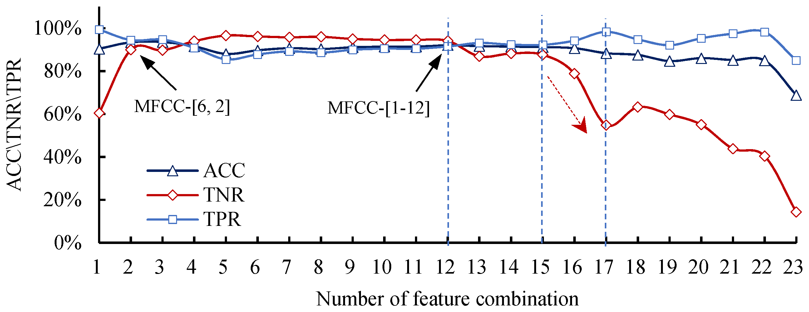
5.1.1. Accuracy of AIEFPC with Different Combinations of MFCC as Sample Feature

To construct different combinations of Mel cepstrum coefficients, we first analyze the importance of the sample features in the prediction process of AIEFPC. According to Equation (2), when N features are selected as sample features, the posterior probability p(y = 1|X) of the AE sample label in AIEFPC is obtained:

$$\ln \frac{p\left(y=1\left|X\right.\right)}{1-p\left(y=1\left|X\right.\right)}={\displaystyle \sum _{n=1}^N{w}_n{x}_n}+b_{\mathrm{N}}$$

(10)

where b_N is the intercept value of AIPEFC.

During the process of analyzing the importance of the features of AIEFPC, for simplification purposes, it is assumed that the sample features and the stress state satisfy a monotonic relationship. There exists a probability value p(y = 1|X) of 0.5 at the critical value, which is the right side of Equation (12), and is equal to zero, so b_N satisfies:

$$b_{\mathrm{N}}=-{\displaystyle \sum _{n=1}^N{w}_n{x}_n^c}$$

(11)

where $x_n^c$ is the n-th sample feature MFCC-n of the sample when the stress state is the critical value.

Substituting Equation (11) into Equation (10), the posterior estimated probability value p(y = 1|X) of the sample label y = 1 is:

$$\ln \frac{p\left(y=1\left|X\right.\right)}{1-p\left(y=1\left|X\right.\right)}={\displaystyle \sum _{n=1}^N{w}_n\left(x_n-x_n^c\right)}$$

(12)

The importance I_n of the sample feature x_n on the training set with M samples is:

$$I_n=\frac{1}{M}{\displaystyle \sum _{m=1}^M\left|w_n\left(x_n^m-x_n^c\right)\right|}$$

(13)

where $x_n^m$ is the n-th sample feature value of the m-th sample on the training set.

We use the average value of MFCC-n of all samples on the training set as $x_n^c$. The importance I_n of the sample feature x_n is:

$$I_n=\left|w_n\left(\overline{x{1}_n}-\overline{x{0}_n}-\overline{x_n}\right)\right|$$

(14)

where $\overline{x{0}_n}$, $\overline{x{1}_n}$ and $\overline{x_n}$ are the average of the MFCC-n of the safe samples, hazardous samples, and all samples in the training set.

The division method of the training set and the test set use the Fold-5 in Figure 7, using the training set samples to obtain the AIEFPC parameter w_n. The statistics result in in the average value of the sample feature MFCC-n on the safe sample set, the hazardous sample set, and all of the sample sets. The importance of the sample feature of AIEFPC when the first 12 coefficient values of the Mel frequency cepstrum as the sample feature are calculated by employing Equation (14), and the absolute importance of the sample features of AIEFPC is shown in Figure 11.

Figure 11 clearly depicts the importance of MFCC-6, MFCC-2, MFCC-1, MFCC-10, MFCC-4, and MFCC-8 in descending order, which is a feature of greater importance in the sample. The feature importance of MFCC-5, MFCC-7, MFCC-9, and MFCC-11 are all 0.9. MFCC-12 and MFCC-3 are the two features with the least importance in the sample.

In order to study the influence of different combinations of MFCC as sample features on the AIEFPC prediction effect, firstly, according to Figure 11, the sample features are arranged based on priority and importance. The combination of MFCC is obtained by sequentially adding a feature, starting from the most important feature, MFCC-6, until all 12 Mel cepstral coefficients are added. Then, the most important features in the sample are sequentially subtracted from the 12 Mel cepstral coefficients to obtain a combination of Mel cepstral coefficients, starting from the most important features. The most important features in the sample are subtracted for obtaining a combination of MFCC, also starting from the most important MFCC-6. We obtained 23 different combinations of MFCC, respectively. Various combinations of MFCC were used as sample feature training to obtain 23 AIEFPCs. By analyzing the ACC, TPR, and TNR of each AIEFPC on the test set, using different combinations of MFCC as sample features in the AIEFPC prediction effect is studied. The combination of MFCC and combination number are shown in

Table 5. Mel cepstrum coefficient combination and combination number.

Number of Feature Combination	MFCC Combine	Number of Feature Combination	MFCC Combine
1	MFCC-[6]	13	MFCC-[2,1,10,4,8,5,7,9,11,3,12]
2	MFCC-[6,2]	14	MFCC-[1,10,4,8,5,7,9,11,3,12]
3	MFCC-[6,2,1]	15	MFCC-[10,4,8,5,7,9,11,3,12]
4	MFCC-[6,2,1,10]	16	MFCC-[4,8,5,7,9,11,3,12]
5	MFCC-[6,2,1,10,4]	17	MFCC-[8,5,7,9,11,3,12]
6	MFCC-[6,2,1,10,4,8]	18	MFCC-[5,7,9,11,3,12]
7	MFCC-[6,2,1,10,4,8,5]	19	MFCC-[7,9,11,3,12]
8	MFCC-[6,2,1,10,4,8,5,7]	20	MFCC-[9,11,3,12]
9	MFCC-[6,2,1,10,4,8,5,7,9]	21	MFCC-[11,3,12]
10	MFCC-[6,2,1,10,4,8,5,7,9,11]	22	MFCC-[3,12]
11	MFCC-[6,2,1,10,4,8,5,7,9,11,3]	23	MFCC-[12]
12	MFCC-[6,2,1,10,4,8,5,7,9,11,3,12]	24

Note: MFCC-[6,2,10,4] indicates that MFCC-6, MFCC-2, MFCC-10, and MFCC-4 are used as sample characteristics.

.

The number in brackets indicates the number of the selected MFCC. For example, MFCC-[6,2] indicates that the sixth and second coefficients of the Mel cepstrum coefficient are used as a sample feature. The results of ACC, TNR, and TPR of AIEFPC on the test set of ad8-5 and bd8-5 are shown in Figure 12.

Figure 12 illustrates that from combination 2 to combination 12, the ACC, TNR, and TPR show no significant change and they are relatively stable, and the accuracy of the three is high. From combination 12 to combination 22, the ACC decreased slowly; however, the decline is not significant. From combination 12 to combination 13, the TNR decreased suddenly, and from combination 16, the TNR significantly decreased; however, TPR and TNR have the opposite trend, and increase in the transition from combination 12 to combination 22. For combination 23, the ACC, TNR, and TPR were significantly lower. The above rules show that increasing the number of MFCC as sample features can make the trained model have a better prediction effect. When the sample lacks high-importance MFCC, the model impact will be seriously affected. This phenomenon is discussed in further detail below.

In combination 1, only MFCC-6 is used as the sample feature. The accuracy of AIEFPC is 90.4%; however, the accuracy of the dangerous sample set is only 60.4%. It can be seen from Figure 5 that MFCC-6 is the MFCC with a preeminent correlation with the stress state. Nevertheless, only using MFCC-6 as a sample feature has a lower prediction accuracy on the hazardous sample set. Compared with combination 1 and combinations 2 to 12, it is evident that the AIEFPC, which combines ASR and ML, uses multiple MFCC of AE as a sample feature and the LR to predict the failure probability of the coal samples, which is better than employing a single MFCC.

As mentioned in Section 4.1, MFCC-4 and MFCC-10 first decrease and then increase with stress and have a low correlation with stress. It can be seen from Table 5 that the sample feature combination 15 has more MFCC-4 and MFCC-10 than the sample feature combination 17. When the sample uses the combination 15 to become the feature combination 17, the TNR of AIEFPC is reduced from 87.6% to 54.9%, and MFCC-4. MFCC-10 plays an essential role in AIEFPC in improving the prediction accuracy of AIEFPC on the hazardous set. It can be seen from Figure 10 that the feature importance of MFCC-4 and MFCC-10 is second only to MFCC-6, MFCC-2, and MFCC-1 among the 12 Mel cepstral coefficient values. The sample feature importance of AIEFPC cannot be judged solely based on the correlation between MFCC and the stress state.

Figure 11 depicts that the sample feature combination 2 selects MFCC-2 and MFCC-6. The ACC, TPR, and TNR of AIEFPC on the test set are 93.4%, 94.4%, and 89.9%, respectively; using MFCC-2 and MFCC-6 as a sample feature has an ideal prediction effect. When sample feature combination 3 to sample feature combination 12 are used as sample features, the minimum values of ACC, TPR, and TNR of AIEFPC are 88.0%, 85.4%, and 89.7%, respectively. AIEFPC has a high predictive ability. Sample feature combination 16, MFCC-6, MFCC-2, MFCC-1, and MFCC-10 are removed from the sample, and MFCC-4, MFCC-8, MFCC-5, MFCC-6, MFCC-7, MFCC-8, and MFCC-9 are the sample features. Although 8 MFCC is selected, the TNR of AIEFPC is only 78.8%, which shows low prediction accuracy on the hazardous sample set. The accuracy of the sample combination 17 to sample combination 23 on the hazardous sample set did not exceed 70%, and the AIEFPC prediction effect was poor. As mentioned in Section 4.1, MFCC-2, MFCC-6, and MFCC-1 are the three most important MFCC in Figure 10. They are also the first 12 values of Mel cepstrum coefficients that are more relevant to the stress state. In constructing AIEFPC by using LR, the feature with high feature importance in the samples is the key factor in determining the prediction effect of AIEFPC.

It can be seen from Figure 11 that when the sample contains features MFCC-2 and MFCC-6, adding other features to the sample, AIEFPC has an excellent predictive effect, and the predictive ability is relatively stable. To study the impact of adding features with a low correlation with the stress state to the AIEFPC prediction results when the sample contains features with high importance and good correlation with the stress state of the coal sample, we add a random noise feature that is not related to the stress state and satisfies the normal distribution in the samples composed of the first 12 Mel cepstrum coefficients to train the model. The average value of the noise feature is 10, and the standard deviation is 10. When the MFCC and noise feature are used together as the sample feature, the noise feature coefficient w value is 3.6 × 10⁻⁵ in the AIEFPC, far less than that of MFCC. That is to say, the noise feature hardly plays a role in the model and can be ignored. The ACC, TNR, and TPR of AIEFPC on the sample set are shown in Figure 13 when the MFCC and noise feature are used as sample features.

It can be seen from Figure 13 that when MFCC is used as a sample feature, the prediction effect of AIEFPC on the sample set has little change after adding the noise feature and adding noise features has little impact on AIEFPC’s prediction ability. When the sample contains features with high importance and a good correlation with the stress state, adding features with a low correlation with the stress state has little impact on the prediction results of AIEFPC. Suppose the predicted effect of AIEFPC is not ideal. In such a case, the sample features with high importance are not included in the sample. The sample features with a strong correlation with the stress state should be obtained by optimizing the parameter extraction process. It is difficult to improve the prediction effect of the model using feature selection. In this paper, all of the first 12 AE Mel-frequency cepstrum coefficients are selected as sample features.

5.1.2. AIEFPC Prediction Results with Traditional Acoustic Emission Parameters as Sample Features

The training set and test set coal sample division, sample label making, training, and prediction AIEFPC process are the same as in Section 5.1.1. The AE wave data are divided into 40 ms segments, and the cumulative hits, cumulative count, and amplitude in the AE segment are used as sample features. The change of the AIEFPC prediction effect is studied when the cumulative hits number, cumulative ring count, and maximum amplitude are used as the sample feature. MFCC is used as the sample feature. The ACC, TPR, and TNR of AIEFPC on the AE sample set of ad8-5 and bd8-5 using cumulative hits, cumulative count, and amplitude as sample features and MFCC-6 as sample features are shown in Figure 14.

According to Figure 14, the cumulative hits, the cumulative count, and the amplitude can be used as the sample features. Compared with using all 12 AE Mel cepstrum coefficients as the sample features, the TPR prediction accuracy on the safe sample set is increased from 91.4% to 99.1%. However, the prediction accuracy is reduced from 92.0% to 88.7%, and the TNR prediction accuracy on the dangerous sample set is reduced from 94% to 53.9%. In practical applications, AIEFPC misinterprets the hazardous samples as safe samples, which may lead to severe consequences, such as disastrous accidents and massive losses, which is unacceptable. Therefore, MFCC, as a sample feature, is more suitable than a cumulative hits, cumulative count, and amplitude.

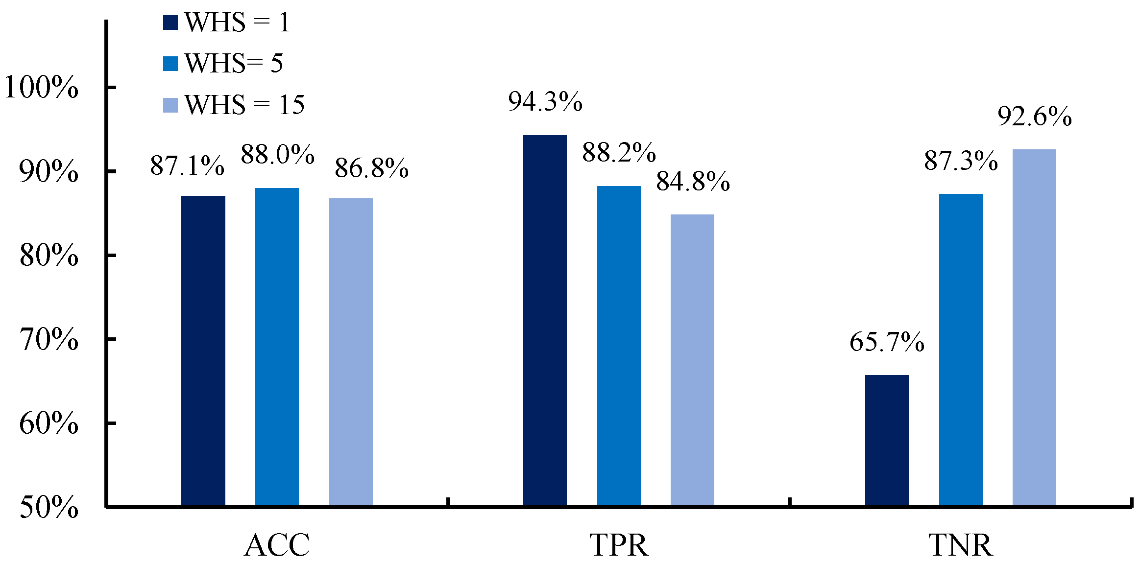
5.2. Influence of Category Weight of Sample on AIEFPC Prediction Effect on the Different Category Sample Set

If AIEFPC mistakenly judges a safe sample with a small stress state as a hazardous sample, it is a false alarm that will issue incorrect waring information. However, if it mistakenly judges a high-stress state sample as safe, it is omitted, causing disasterous accidents and huge losses. Improving the prediction accuracy of the AIEFPC on the hazardous samples set will help improve the application values of the AIRFPC in coal and rock failure monitoring. The LR can improve the accuracy of the high-cost category by increasing the category weight value with higher cost and solving the binary classification problem with different category loss costs. The log-likelihood function of LR considering the category weight is:

$$L\left(\beta \right)={\displaystyle \sum _{i=1}^m\left[C_1·y_i\log \left[p\left(y=1\left|x_i\right.\right)\right]+C_0(1-y_i)\log (1-p\left(y=1\left|x_i\right.\right))\right]}$$

(15)

C₁ and C₀ are the category weight values of the hazardous sample and the safe sample. Use the class_weight of the Logistic Regression class in sklearn to set the category weight of the sample.

The training set uses the training set and test set division method in Fold-5 in Figure 7, the category weight of the safe sample is set to 1, and 30 logarithmic distribution values between 0.125 and 16 are taken as the category weight of the hazardous sample. Thirty AIEFPC with the category weight of hazardous samples are trained. Figure 15 is the cloud chart of the probability value of AIEFPC prediction coal sample aD8-5 in the uniaxial compression failure process.

It can be seen from Figure 15 that the probability values of AIEFPC prediction samples with different weight values of hazardous samples are dangerous samples, and the probability values increase with the increase in the stress state. The greater the category weight of the hazardous sample, the greater the probability value of AIEFPC predicting samples being hazardous samples, so more samples will be predicted as hazardous samples. The prediction accuracy of AIEFPC on the hazardous sample set will be increased, and the accuracy of the safe sample set will be reduced.

It can be seen from Table 3 that the TNR of Fold-4 is 65.7%, which is the lowest group in the five-fold cross-validation. We use the Fold-4 training set and test set coal sample division method by setting different category weight values of the hazardous sample to study the impact of the sample category weight values on AIEFPC’s prediction results on different category sample sets. When the category weight value of the safe sample is set to 1, and the category weight values of the hazardous sample are 1, 5, and 15, respectively, AIEFPC predicts the results of ACC, TNR, and TPR on the test set aD8-4 and bD8-4 samples, as shown in Figure 16.

As shown in Figure 16, when the category weights of the hazardous sample are 1, 5, and 15, respectively, the ACC of AIEFPC on the test set is 87.1%, 88.0%, and 86.8%, the prediction accuracy for the hazardous sample set is 65.7%, 87.3%, and 92.6%, and the accuracy for the safe sample set is 94.3%, 88.2%, and 94.8%, respectively. As the category weight of the hazardous samples increases, the ACC of AIEFPC first increases and then decreases. The accuracy of the safe sample set of the AIEFPC decreases as the category weight of the hazardous samples increases. The prediction accuracy for the hazardous sample increases when the category weight of the hazardous samples increases.

6. Conclusions

This paper presents unique applications of machine learning (ML) and automatic speech recognition (ASR) for evaluating the failure possibility of coal samples by employing acoustic emission (AE) as the core technology. The Mel-frequency cepstrum coefficient (MFCC) approach in the ASR methodology was used to extract the MFCC of AE as the sample features. The logistic regression (LR) of ML was employed to construct the artificial intelligence evaluation of the failure probability of coal (AIEFPC). A five-fold cross-validation method was used to evaluate the AIEFPC prediction effect and compared with the traditional AE parameters, and different combinations of MFCC were used as sample features. The influence of the category weight of the sample on the prediction effect of AIEFPC on various sample set was discussed. The following conclusions were drawn:

• AIEFPC based on ASR and ML can predict the AE sample label based on the MFCC of the 40 ms AE segment at any time. The maximum prediction accuracy is 92.0%, while the minimum value is 85.2%.
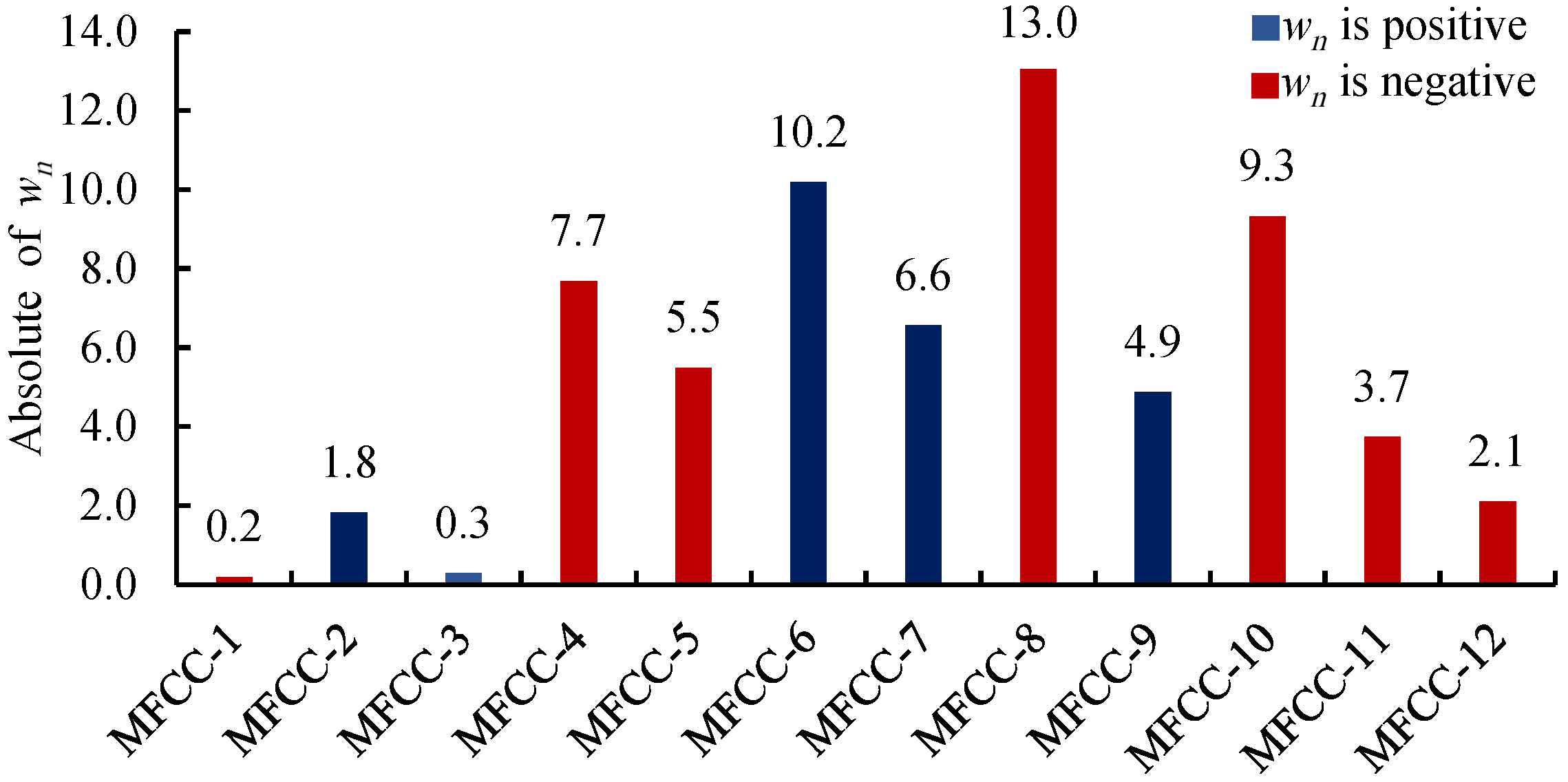
• The mean value of MFCC-n of non-hazardous samples, hazardous samples, and all samples and the feature parameters w_n of AIEFPC can be used to calculate the sample feature importance.
• In the process of using the ML to construct AIEFPC, the sample contains multiple sample features with high importance, which is a critical factor in determining the predictive effect of the AIEFPC.
• When the sample contains the features with high importance, adding features with a low correlation with the stress state has little impact on the prediction results of AIEFPC constructed by ML and ASR. In this paper, all of the first 12 Mel-frequency cepstrum coefficients were selected as sample features.
• When using cumulative hits, cumulative count, and amplitude as sample features, AIEFPC has low prediction accuracy on the hazardous sample set. The MFCC is better than cumulative hits, cumulative count, and amplitude as sample features.
• As the category weight of the hazardous samples increases, the ACC of AIEFPC first increases, followed by a decrease. The accuracy of the safe sample set of AIEFPC decreases as the category weight of the hazardous samples increases.

References

1. Yong, I.; Rangang, Y.; Yin, Z.; Xinbo, Z. Application of Acoustic Emission Characteristics in Damage Identification and Quantitative Evaluation of Limestone. Adv. Eng. Sci. 2020, 52, 115–122. [Google Scholar]
2. Guangcai, W.; Jiangong, L.; Yinhui, Z.; Guichun, L. Preliminary study on the application conditions of acoustic emission monitoring dynamic disasters in coal and rock. J. China Coal Soc. 2011, 36, 278–282. [Google Scholar]
3. He, S.; Song, D.; Li, Z.; He, X.; Chen, J.; Li, D.; Tian, X. Precursor of Spatio-temporal Evolution Law of MS and AE Activities for Rock Burst Warning in Steeply Inclined and Extremely Thick Coal Seams under Caving Mining Conditions. Rock Mech. Rock Eng. 2019, 52, 2415–2435. [Google Scholar] [CrossRef]
4. Wang, C. Identification of early-warning key point for rockmass instability using acoustic emission/microseismic activity monitoring. Int. J. Rock Mech. Min. 2014, 71, 171–175. [Google Scholar] [CrossRef]
5. Vilhelm, J.; Rudajev, V.; Ponomarev, A.V.; Smirnov, V.B.; Lokajíček, T. Statistical study of acoustic emissions generated during the controlled deformation of migmatite specimens. Int. J. Rock Mech. Min. 2017, 100, 83–89. [Google Scholar] [CrossRef]
6. Gong, Y.; Song, Z.; He, M.; Gong, W.; Ren, F. Precursory waves and eigenfrequencies identified from acoustic emission data based on Singular Spectrum Analysis and laboratory rock-burst experiments. Int. J. Rock Mech. Min. 2017, 91, 155–169. [Google Scholar] [CrossRef]
7. Ohno, K.; Ohtsu, M. Crack classification in concrete based on acoustic emission. Constr. Build. Mater. 2010, 24, 2339–2346. [Google Scholar] [CrossRef]
8. Liu, Y.; Liu, S.; Li, Z.; Li, X.; Chen, P.; Yang, X. Energy distribution and fractal characterization of acoustic emission (AE) during coal deformation and fracturing. Measurement 2019, 136, 122–131. [Google Scholar] [CrossRef]
9. Zeng, W.; Yang, S.; Tian, W. Experimental and numerical investigation of brittle sandstone specimens containing different shapes of holes under uniaxial compression. Eng. Fract. Mech. 2018, 200, 430–450. [Google Scholar] [CrossRef]
10. Zhang, Y.; Zhao, G.; Li, Q. Acoustic emission uncovers thermal damage evolution of rock. Int. J. Rock Mech. Min. 2020, 132, 104388. [Google Scholar] [CrossRef]
11. Zhao, K.; Yang, D.; Gong, C.; Zhuo, Y.; Wang, X.; Zhong, W. Evaluation of internal microcrack evolution in red sandstone based on time–frequency domain characteristics of acoustic emission signals. Constr. Build. Mater. 2020, 260, 120435. [Google Scholar] [CrossRef]
12. Gu, Q.; Ma, Q.; Tan, Y.; Jia, Z.; Zhao, Z.; Huang, D. Acoustic emission characteristics and damage model of cement mortar under uniaxial compression. Constr. Build. Mater. 2019, 213, 377–385. [Google Scholar] [CrossRef]
13. Geng, J.; Sun, Q.; Zhang, Y.; Cao, L.; Zhang, W. Studying the dynamic damage failure of concrete based on acoustic emission. Constr. Build. Mater. 2017, 149, 9–16. [Google Scholar] [CrossRef]
14. Zhou, D.; Zhang, G.; Wang, Y.; Xing, Y. Experimental investigation on fracture propagation modes in supercritical carbon dioxide fracturing using acoustic emission monitoring. Int. J. Rock Mech. Min. 2018, 110, 111–119. [Google Scholar] [CrossRef]
15. Zhu, X.; Xu, Q.; Zhou, J.; Tang, M. Experimental study of infrasonic signal generation during rock fracture under uniaxial compression. Int. J. Rock Mech. Min. 2013, 60, 37–46. [Google Scholar] [CrossRef]
16. Zhu, Q.; Li, D.; Han, Z.; Li, X.; Zhou, Z. Mechanical properties and fracture evolution of sandstone specimens containing different inclusions under uniaxial compression. Int. J. Rock Mech. Min. 2019, 115, 33–47. [Google Scholar] [CrossRef]
17. Li, J.; Hu, Q.; Yu, M.; Li, X.; Hu, J.; Yang, H. Acoustic emission monitoring technology for coal and gas outburst. Energy Sci. Eng. 2019, 7, 443–456. [Google Scholar] [CrossRef] [Green Version]
18. Gupta, V.; Juyal, S.; Hu, Y.C. Understanding human emotions through speech spectrograms using deep neural network. J. Supercomput. 2022, 78, 6944–6973. [Google Scholar] [CrossRef]
19. Ganne, P.; Vervoort, A.; Wevers, M. Quantification of pre-peak brittle damage: Correlation between acoustic emission and observed micro-fracturing. Int. J. Rock Mech. Min. 2007, 44, 720–729. [Google Scholar] [CrossRef]
20. Jiang, D.; Xie, K.; Chen, J.; Zhang, S.; Tiedeu, W.N.; Xiao, Y.; Jiang, X. Experimental Analysis of Sandstone Under Uniaxial Cyclic Loading Through Acoustic Emission Statistics. Pure Appl. Geophys. 2019, 176, 265–277. [Google Scholar] [CrossRef]
21. Tirumala, S.S.; Shahamiri, S.R.; Garhwal, A.S.; Wang, R. Speaker identification features extraction methods: A systematic review. Expert. Syst. Appl. 2017, 90, 250–271. [Google Scholar] [CrossRef]
22. Randall, R.B.; Antoni, J.; Smith, W.A. A survey of the application of the cepstrum to structural modal analysis. Mech. Syst. Signal Process. 2019, 118, 716–741. [Google Scholar] [CrossRef]
23. Randall, R.B. A history of cepstrum analysis and its application to mechanical problems. Mech. Syst. Signal Process. 2017, 97, 3–19. [Google Scholar] [CrossRef]
24. Honglei, W.; Song, D.; Xueqiu, H.; Zhenlei, L.; Liming, Q.; Shirui, L. Acoustic Emission characteristics of coal failure using Automatic Speech Recognition methodology analysis. Int. J. Rock Mech. Min. 2020, 136, 104472. [Google Scholar]
25. Pu, Y.; Apel, D.B.; Wei, C. Applying Machine Learning Approaches to Evaluating Rockburst Liability: A Comparation of Generative and Discriminative Models. Pure Appl. Geophys. 2019, 176, 4503–4517. [Google Scholar] [CrossRef]
26. Sun, D.; Wen, H.; Wang, D.; Xu, J. A random forest model of landslide susceptibility mapping based on hyperparameter optimization using Bayes algorithm. Geomorphology 2020, 362, 107201. [Google Scholar] [CrossRef]
27. Suman, A.; Kumar, C.; Suman, P. Early detection of mechanical malfunctions in vehicles using sound signal processing. Appl. Acoust. 2022, 188, 108578. [Google Scholar] [CrossRef]
28. Ohlmacher, G.C.; Davis, J.C. Using multiple logistic regression and GIS technology to predict landslide hazard in northeast Kansas, USA. Eng. Geol. 2003, 69, 331–343. [Google Scholar] [CrossRef]
29. Li, Z.; Wang, E.; Ou, J.; Liu, Z. Hazard evaluation of coal and gas outbursts in a coal-mine roadway based on logistic regression model. Int. J. Rock Mech. Min. 2015, 80, 185–195. [Google Scholar] [CrossRef]
30. Cao, D.; Gao, X.; Gao, L. An Improved Endpoint Detection Algorithm Based on MFCC Cosine Value. Wirel. Pers. Commun. 2017, 95, 2073–2090. [Google Scholar] [CrossRef]
31. Zhihua, Z. Machine Learning; Tsinghua University Press: Beijing, China, 2016. [Google Scholar]
32. Hang, L. Statistical Learning Method; Tsinghua University Press: Beijing, China, 2012. [Google Scholar]
33. Pedregosa, F.; Varoquaux, G.; Gramfort, A.; Michel, V.; Thirion, B.; Grisel, O.; Blondel, M.; Prettenhofer, P.; Weiss, R.; Dubourg, V.; et al. Scikit-learn: Machine Learning in Python. J. Mach. Learn. Res. 2011, 12, 2825–2830. [Google Scholar]
34. Zhang, H.; Li, R.; Cai, Z.; Gu, Z.; Heidari, A.A.; Wang, M.; Chen, H.; Chen, M. Advanced orthogonal moth flame optimization with Broyden–Fletcher–Goldfarb–Shanno algorithm: Framework and real-world problems. Expert. Syst. Appl. 2020, 159, 113617. [Google Scholar] [CrossRef]
35. Ciyou, Z.; Byrd, R.H.; Lu, P.; Nocedal, J. Algorithm 778: L-BFGS-B: Fortran Subroutines for Large-Scale Bound-Constrained Optimization. Trans. Math. Softw. 1997, 23, 550–560. [Google Scholar]
36. Qi, C.; Fourie, A.; Du, X.; Tang, X. Prediction of open stope hangingwall stability using random forests. Nat. Hazards 2018, 92, 1179–1197. [Google Scholar] [CrossRef]
37. Xue, Y.; Bai, C.; Qiu, D.; Kong, F.; Li, Z. Predicting rockburst with database using particle swarm optimization and extreme learning machine. Tunn. Undergr. Space Technol. 2020, 98, 103287. [Google Scholar] [CrossRef]
Figure 1. Methodology adopted for constructing and applying AIEFPC model by coupled use of machine learning and automatic speech recognition.
Minerals 12 01548 g001
Figure 2. Waveform, segmentation, feature extraction, and labeling of AE signal.
Minerals 12 01548 g002
Figure 3. AE sample segmentation.
Minerals 12 01548 g003
Figure 4. Extraction scheme of MFCC for the AE of coal [24].
Minerals 12 01548 g004
Figure 5. Schematic diagram of experimental setup.
Minerals 12 01548 g005
Figure 6. Variation of MFCC of AE with respect to stress state of the coal specimen No. aD8-5 subjected to uniaxial compression.
Minerals 12 01548 g006
Figure 7. Absolute value of the coefficient wn corresponding to MFCC-n in AIEFPC. The blue bars indicate wn is positive while red indicates wn is negative.
Minerals 12 01548 g007
Figure 8. Coal samples of the train set and test set of five-fold cross-validation.
Minerals 12 01548 g008
Figure 9. Probability value that AIEFPC predicts the AE sample is a hazard sample at an aD8-5 coal sample during uniaxial compression.
Minerals 12 01548 g009
Figure 10. Probability distribution of AIEFPC prediction for the AE sample hazardousness corresponding to different stress states.
Minerals 12 01548 g010
Figure 11. Absolute importance of sample features of AIEFPC.
Minerals 12 01548 g011
Figure 12. ACC, TNR, and TPR of 23 AIEFPC models obtained by different combinations of MFCC are selected as the AE sample feature on the sample set of coal samples ad8-5 and bd8-5.
Minerals 12 01548 g012
Figure 13. ACC, TNR, and TPR of AIEFPC on the sample set when using MFCC and noise features as sample features.
Minerals 12 01548 g013
Figure 14. ACC, TPR, and TNR of AIEFPC on the AE sample set of ad8-5 and bd8-5, using cumulative hits, cumulative count, and amplitude as sample features and MFCC-6 as sample features.
Minerals 12 01548 g014
Figure 15. Cloud chart of the probability value of AIEFPC with different category weights of hazardous sample on the test set aD8-5 samples at different time.
Minerals 12 01548 g015
Figure 16. Category weight of safe sample is set to 1, and category weights of hazardous sample are 0.5, 5, and 15, respectively. The ACC, TPR, and TNR of AIEFPC on the test set aD8-4 and bD8-4 samples. WHS is the category weight values of the hazardous sample.
Minerals 12 01548 g016