
Predictive Mapping of Prospectivity for Gold in the Central Portion of the Tapajós Mineral Province, Brazil

1
Economic Geology Division, Geological Survey of Brazil (SGB/CPRM), Belém 66095-110, Brazil
2
Institute of Geosciences, University of Campinas (UNICAMP), Campinas 13083-855, Brazil
*
Author to whom correspondence should be addressed.
Minerals 2023, 13(11), 1432; https://doi.org/10.3390/min13111432
Submission received: 11 October 2023
/
Revised: 4 November 2023
/
Accepted: 6 November 2023
/
Published: 12 November 2023
(This article belongs to the Special Issue Footprints of Mineral Systems)
Abstract
:This work aims to model mineral prospectivity for intrusion–related gold deposits in the central portion of the Tapajós Mineral Province (TMP), southwestern Pará state. The scope includes experimentation and evaluation of knowledge and data-driven methods applied to multisource data to predict potential targets for gold mineralization. The radiometric data processing allowed to identify a hydrothermal alteration footprint of known gold deposits, providing information in regions with little or no field data available. The aeromagnetic data analysis prompted the identification of high magnetic zones, which are probably related to hydrothermal fluid transport. Linear features extracted from digital elevation data revealed an NNW–SSE general trend, which is consistent with the main structural control of deposits. The data were integrated through three modeling techniques—fuzzy logic (knowledge-driven), weights of evidence (WofE, data-driven), and a machine learning algorithm (SVM, data-driven)—resulting in three prospective models. In all models, the majority of indicated prospective regions coincide with the known deposits. The results obtained in the models were combined to generate an agreement map, which mapped the overlapping of their highest prospective scores, indicating new areas of prospective interest in the central portion of the TMP.
1. Introduction
The growing demand in the mineral sector for the discovery of new mineral deposits has been a relevant issue for the conception of predictive mapping models for mineral prospectivity. Such models involve the analysis and integration of evidential maps derived from multi-source geoscientific datasets to delineate and classify areas favorable to the presence of undiscovered mineral deposits [1].
For mineral prospectivity modeling, geocomputational methods guided by specialized knowledge (knowledge-driven), available data (data-driven), or hybrid methods are employed [1,2]. Knowledge-driven methods are suitable in areas with few exploration targets and limited information, as well as where there is greater knowledge of mineralization components. Data-driven methods are generally applied when there is a robust collection of data with a considerable number of known mineral occurrences [1].
Fuzzy logic (knowledge-driven) and the weights of evidence (WofE, data-driven) are commonly used methods in geological modeling (e.g., [3,4]). The use of data-driven methods based on machine learning algorithms is a growing trend. These algorithms can recognize complex spatial patterns, learn from them, and autonomously indicate the presence of these patterns in specific areas [5,6]. The simultaneous application and comparison of results obtained with different methods at exploration boundaries are also pervasive in the specialized literature [7,8,9,10,11].
Mineral prospectivity studies have a conceptual basis in the analysis of knowledge about mineral deposits, their environments, and the factors influencing their formation. The mineral systems approach [12] provides a comprehensive view of mineral deposit formation and evaluates critical factors in their formation, including source, metal transport, deposition, and post-depositional enrichment processes. Furthermore, geological processes operate at various spatial and temporal scales, encompassing common aspects of different types of deposits. Mineral systems are divided into orthomagmatic, hydrothermal, and sedimentary systems [13], which can overlap, considering the tectonic and geodynamic evolution of the region.
The Tapajós Mineral Province (TMP), the focus of this study, is one of Brazil’s most important polymetallic provinces, particularly known for gold deposits hosted in granitoid bodies. It is a vast region with high economic potential but limited geological and metallogenetic knowledge (greenfield). The TMP lacks detailed geological knowledge and analyses of mineral potential using modern data and methods to identify potential mineral targets. Indicative work on favorable zones for gold mineralization in the TMP has shown promising results [14,15,16,17]. With the increasing development of geotechnologies, coupled with the addition of new data characterizing different deposits, predictive models can be improved to indicate potential areas with greater precision.
In this context, this study aims to predict prospectivity on a semi-detailed scale, indicating areas favorable for gold mineralization related to intrusions in the central portion of the TMP, using knowledge-driven, data-driven methods, and machine learning algorithms to compare them and contribute to the definition of new strategies for mineral exploration in the region.
2. Geological Setting
The TMP is located in the central-southern part of the Amazonian Craton, corresponding to the Tapajós domain [18,19] of the Tapajós-Parima (or Ventuari-Tapajós) tectonic province [20,21] (Figure 1a,b). The region consists of Archean and Paleoproterozoic terranes that were tectonically stabilized around 1.0 Ga [22,23]. Their origin is associated with the craton’s structuring through accretion events and crustal shortening of mobile belts and magmatic arcs predominantly oriented NNW-SSE relative to an Archean protocraton [20,21,22]. In the southwest of the TMP, basement rocks outcrop, and are metamorphosed from low to high grade and with variable ductile deformation. In the southeast and central-south regions, granitoids occur with weak to moderate ductile deformation, which is related to the NW–SE shear zones. In the eastern and northeastern portions, rocks have mainly undergone brittle deformation. The gradual variation in the exposed crustal level in the province is also observed through variations in mineralization controls [14,24,25,26].
The tectonic evolution of the TMP occurred during the Paleoproterozoic. The lithological associations in the study area are illustrated in Figure 2. The basement of the province is primarily composed of rocks from the Jacareacanga Group (2.1–2.87 Ga) and the Cuiú–Cuiú Complex (2.03–2.0 Ga) [20,30], and is related to the early stages [31] of the formation of the Cuiú–Cuiú magmatic arc [14,32,33,34,35]. Among the oldest units are (i) the Comandante Arara Formation (ca. 2.0 Ga) [36], which has a more evolved calc-alkaline signature and represents the maturation of the arc in distal regions [37], and (ii) the Castelo dos Sonhos Formation, with auriferous metaconglomerates and metarenites of fluvial origin, deposited between 2.01 and 2.05 Ga [38,39], outcropping in the extreme southeast of the TMP and believed to be remnants of a rift or foreland-type basin [31,37].
Following this phase, more distal magmatic events occurred, characterized by high-potassium calc-alkaline to shoshonitic signatures, which generated rocks of the Vila Riozinho Formation and the Creporizão Suite batholiths between 2.0 and 1.95 Ga [35,37,40,41]. The São Jorge Antigo (1.98 Ga, [40]) and Pindobal (1.94 Ga, [42]) granites are correlated with this suite, whose batholiths are elongated due to emplacement along the NW-SE shear zones.
Between 1.90 and 1.89 Ga, magmatic pulses produced the granitoids of the Tropas Suite [31] and the São Jorge Jovem granite [43]. The granitoids of the Tropas suite have a less evolved calc-alkaline signature. They may represent a possible island arc related to subduction [18,30] or a late post-collisional evolution relative to the Cuiú–Cuiú orogeny [14,35].
This episode was followed by (i) significant post-orogenic granitogenesis, represented by the Parauari Suite granitoids (1.89–1.87 Ga, [20,40]), (ii) intracontinental basic magmatism with intrusions of gabbroic bodies from the Ingarana Suite and their equivalents (1.88 Ga, [31]), and (iii) late-to-post-tectonic anorogenic magmatism in an extensional setting (Uatumã magmatism—1.89–1.87 Ga), with alkaline (Maloquinha Suite), felsic (Salustiano, Aruri, and Moraes Almeida Formations), and intermediate to mafic (Bom Jardim Formation) compositions [31,44]. Most of the granitoids are controlled by regional NW–SE-trending faults, and some mafic bodies are elongated in an E–W and NW–SE direction, characterized by faulted contacts with other units [31,37].
The geological evolution of the province settles with the establishment of intracratonic estaterian sedimentary basins (Novo Progresso and Coatá Formations) associated with alkaline magmatism (Crepori Diabase, Porquinho Granite) and a mafic magmatism event around 1190 Ma, after a hiatus of about 600 Ma (Cachoeira Seca Suite), composed of olivine gabbros, olivine gabronorites, olivine diabases, and troctolites [31,45,46].
Structures, Metallogeny, and Gold Mineralization
The structural framework of the TMP suggests mutually compressive and extensional deformation, occurring in both ductile and ductile–brittle to brittle regimes. The regional structural orientation is primarily NNW–SSE to NW–SE [47]. Santos [48] identified three deformation and thermotectonic events involving the mobilization and accretion of magmatic arcs on a regional scale during the Paleoproterozoic.
The first event (2005–1997 Ma [47]) generated thrust faults with a NNE–SSW orientation and NW–SE, N–S, and NE–SW lineaments, which were overprinted by the subsequent event. The second event (1970–1950 Ma [47]) produced brittle shear zones with primary orientations of NW–SE and NNW–SSE, which are the most prominent in the TMP. The third event (ca. 1900 Ma [30]) created ductile–brittle shear zones with a NNE–SSW orientation, accompanied by auriferous quartz veins. Progressive deformation altered and reactivated NW–SE and WNW–ESE shear zones. A younger extensional brittle event, related to NW-SE shearing [26,48], is manifested as extensive E–W and ENE–WSW lineaments in the central-eastern part of the TMP. Subsequent deformation events produced brittle structures and/or were associated with reactivations of older structures, favoring the intrusion of Cambrian mafic dikes [47].
The TMP encompasses numerous magmatic–hydrothermal deposits of gold associated with Ag, Cu, Pb, Zn, Bi, and Mo, with mineralizations of various types and styles, representing distal, proximal, or dome portions, which are deep or shallow parts of a structurally controlled mineral system. The primary mineralization occurs in quartz veins and, secondarily, in stockwork and disseminations, with all three forms eventually occurring simultaneously (e.g., São Jorge and Cantagalo). Gold is associated with quartz and sulfides (mainly pyrite and chalcopyrite, and subordinately sphalerite, galena, and pyrrhotite), either as sub-microscopic inclusions or in microfractures (e.g., Tocantinzinho, Batalha, and São Jorge). The deposits typically have well-developed hydrothermal alteration halos (e.g., São Jorge, Palito), with fissure alteration (e.g., Cuiú–Cuiú, Batalha), and sericitic alteration zones are most directly associated with mineralization [47]. Ore bodies are primarily located within structures such as shear zones and have a strong spatial correlation with the emplacement of mafic dikes along these structures at contact zones.
3. Materials and Methods
To assess methods for predictive mineral prospectivity mapping in the TMP, this study involved the following stages: (i) selection of the dataset, (ii) data processing and generation of evidential themes, (iii) prospectivity modeling using various integration techniques, and (iv) model validation. Figure 3 illustrates the details of these stages.
The approach to characterizing mineral deposits was developed following the concept of a mineral system, which evaluates the significance of numerous geological processes for the formation and preservation of deposits, across all scales of observation [12,49,50,51,52].
3.1. Dataset
The data primarily come from the Geological Survey of Brazil and include geological and mineral resource maps, aerogeophysical data (radiometrics and magnetometry), and remote sensing data (digital elevation model—DEM). A total of 21 primary gold occurrence points were selected for training and testing the prospectivity models, with the inclusion of 21 non-deposit points generated randomly. These non-deposit points were distributed at a minimum distance of 12 km from any known deposit point and 7 km from each other. Such control criteria are employed to ensure that the marked points are not coincident or too close to known deposit locations. This is based on the assumption that locations near existing mineral deposits are likely to have similar multivariate spatial data signatures as deposit sites, which could jeopardize the results. Table 1 shows the characteristics of the main prospects in the study area, which are used here as training points. Although the number of training points is small relative to the analyzed area, balancing the dataset improves prediction accuracy, especially in machine learning-based classifiers, compared to imbalanced datasets. Carranza and Laborte [53] demonstrated the successful applicability of various mineral potential modeling tools, including ML methods that require a large amount of training data, using few deposit points (e.g., [3,54,55,56,57]).
3.2. Data Processing
The availability of data and the geological knowledge of the region are heterogeneous. Most of the known deposits are concentrated in the eastern part, while the central part is less explored. To enhance information and reduce subjectivity in the identification of new features important for the mineralization context, statistical and semi-automatic methods were employed.
Aerogeophysical data were integrated into a single database, and grids were interpolated using the minimum curvature method [71] into cells of 125 m. Radiometric channels were verified, and variables with inconsistent physical behavior for natural radiation sources were removed to reduce the impact of these values in mathematical operations between channels.
To map hydrothermal alteration zones, parameters (such as F), anomalous potassium (Kd), anomalous uranium (Ud), and the eTh/K ratio were calculated. The joint analysis of these parameters helps identify alteration zones associated with the presence of K-feldspar and/or sericite/muscovite, such as potassic and phyllic alteration. The F parameter (K × (eU/eTh)) highlights the simultaneous abundance of potassium and uranium in relation to thorium, and anomalous values are good indicators of altered rocks (Efimov cited in Gnojek and Přichystal [72]). This parameter allows the distinction between zones of hydrothermal alteration in strongly weathered areas and has been widely used in identifying mineralization related to these zones (e.g., [73,74,75,76]). The Kd and Ud parameters indicate anomalous concentrations obtained by normalizing K and eU with eTh, calculating the ideal values Ki ((Kmean/eThmean) × eTh) and Ui ((Umean/eThmean) × eTh), and computing the deviation of measured values from these ideals (Kd = ((K − Ki)/Ki); Ud = ((U − Ui)/Ui)) [77,78]. The data are previously classified into gamma spectrometric domains with relatively homogeneous signatures. In heterogeneous areas, the calculation of Ki and Ui results in false enhancements. The eTh/K ratio has been used in mapping hydrothermal alteration zones (e.g., [79,80]) due to the observation that eTh mobility is abnormally low compared to K and eU in hydrothermal processes. It is a valuable exploration vector in magmatic–hydrothermal deposit settings [81], providing a more accurate indication of the extent of alteration and minimizing the influence of naturally K-rich felsic intrusions that can mask deposit signatures ([82], among others).
Magnetometric data were reduced from the International Geomagnetic Reference Field (IGRF), micro-leveled, and interpolated to generate the anomalous magnetic field (AMF) map. The reduction to the pole (RTP—[83]) filter was applied to the AMF map to reduce the influence of induced magnetic fields and to centralize anomalies over their sources. Due to instability in low magnetic latitudes [84], the RTP filter was first tested on synthetic 3D models (as proposed by Bongiolo [85]) and generated using the open source MATLAB-based GRAV MAG PRISM program [86], following the geometric and magnetic parameters shown in Figure 4. The evaluated prisms represent magnetic bodies at different depths in the crust, with geographic positioning and magnetic field conditions (i) in the study area, (ii) reduced to the pole in the study area, and (iii) at the Earth’s magnetic pole.
To verify the continuity of structures in depth, attenuate high spatial frequency signals, and minimize the influence of shallow sources, upward continuation filters were applied [87,88]. The following enhancement filters were applied and tested on the continued data: (i) first vertical derivative (1Dz—[89,90]); (ii) analytic signal amplitude (ASA—[91,92,93,94]); (iii) total horizontal gradient (GHT or THDR—[95,96]); (iv) tilt angle (ISA or TDR—[97]); (v) tilt angle of the total horizontal gradient (TAHG—[98]). These filters improve magnetic responses and highlight subtle anomalies more accurately. Additionally, magnetic worm products were generated on upward continuations to separate shallow high-frequency data from deeper low-frequency data, highlighting edge features. This product helps reduce ambiguity in interpretation and provides information about the overall shape and relative depth of edges, such as faults and geological contacts [99].
The DEM data were processed for the automatic delineation of linear features. Shaded relief images were generated at illumination azimuths of 0°, 45°, 90°, and 135°, which were subsequently overlaid on a multi-directional illumination map, enabling a three-dimensional perception, and minimizing false trends from artificial lighting. The “LINE” algorithm, part of the PCI Geomatica platform (2018, PCI Geomatics Enterprises Inc., Markham, Ontario, Canada), performs processing in three steps: (i) edge detection; (ii) thresholding; (iii) curve extraction. These steps result in the detection of linear patterns in an image and their automatic conversion into vector segments [100].
3.3. Mineral Prospectivity Modelling
The conception of prospectivity maps requires numerous classes of geoscientific information to be spatialized in a GIS environment and combined with various mathematical and logical operations. Mappable criteria indicate the critical parameters (geological processes) of the studied mineral system, which are translated into layers of evidence that result in the classification of promising target areas for future exploration [1,2].
Based on the critical components discussed by Hagemann et al. [13], three critical elements were adopted for mapping the footprints of the mineral system in the TMP: (i) the source of energy, metals, and fluids; (ii) fluid migration pathways; (iii) concentration and deposition processes. From these elements, and based on the theoretical understanding of the TMP’s gold magmatic–hydrothermal system, geological processes and their mappable criteria were established. Spatial proxies (evidence layers) were obtained and pre-processed as described in Section 3.2.
Mineral potential modeling can be achieved by an empirical (data–driven), conceptual (knowledge–driven), or hybrid approach [1,2]. Empirical approaches are applied in areas with limited and poorly distributed data and few known deposits, relying on prior geological knowledge of the study area. Conceptual approaches are used in well-explored areas with robust and well-distributed data, using known mineralized sites as control points. In this study, to examine and compare the results obtained from each approach, the evidence layers were combined using three different integration methods: a knowledge-driven (fuzzy logic) approach and two data-driven approaches, one probabilistic (weights of evidence) and one based on a machine learning algorithm (SVM).
Fuzzy logic [2,3,4,101,102,103,104] is a mathematical tool that converts the probability of a variable into a continuous series of possibilities using fuzzy membership functions, where values are distributed from a midpoint (membership) and spread from there. For the integration of evidence layers, fuzzy OR (logical union) and GAMMA (a combination of the fuzzy PRODUCT and SUM operators) operators were used. Details on fuzzy functions and operators can be found in [105,106].
The weights of evidence (WofE) method, or Bayesian logic, works with parameters estimated from the statistics of the data. Following the procedure described by [2], the method was used to define weights W+ and W− for each of the classes in the evidence layers and the contrast C, defined as the difference between the weights. The evidence layers with relevant weights concerning the deposits are combined, considering the interaction between the measured probabilities in the areas of the layers and the known deposits, both a priori and a posteriori. The method assumes conditional independence between events, and the probability of finding new ore bodies generally increases with the inclusion of new information and the calculation of weights.
The support vector machines (SVM) method [7,107] consists of a set of supervised learning algorithms based on the statistical learning theory [108]. The dataset used is labeled with known class labels, and the algorithm is trained to project an ideal linear hyperplane that optimizes the distance between the two closest sample points (support vectors) to separate multiple classes. The larger the distance between the support vectors, the lower the classification error [109,110].
To explain the method, consider a training set with two separable classes (e.g., mineralized and non-mineralized zones), with samples represented as , where belongs to an n-dimensional space, and is a class label equal to 1 for one class and −1 for the other class (i.e., ) [111]. The classification hyperplanes satisfy the equation , where ; and are parameters of the hyperplane’s decision function [112]. The decision function is given by , where is a function equal to , if ; , se ; and , if , defining margin hyperplanes ( and ) and the central hyperplane (). The parameters e are obtained with , which is subject to . This optimization is constrained, and the solution is given by Lagrange multipliers, as per the equation . This function is minimized with respect to e and maximized with respect to . The multiplier is determined by the equation , which is subject to e . Thus, the rule for classifying based on the ideal hyperplane is determined by the function .
Non-linear datasets are converted into linear ones by transferring input data to a higher-dimensional feature space using kernel functions. In this work, the radial basis function (rbf) kernel function was selected because it has lower error rates compared to others [107], and it requires simple parameters for geoscientific data applications, namely the parameter C (balancing errors, margin width, and the number of support vectors) and the parameter γ (related to the width of the distribution and optimized for better results).
To properly assess the prospective model’s performance, the F1 score [113] was used, considering both recall (R) and precision (P). R is the percentage of mineralized points classified as true positives (tp) relative to the total number of samples in the positive class (tp and false negatives—fn). P is the ratio of tp to the total number of samples classified as positive (i.e., tp and false positives—fp). The score is obtained by calculating the harmonic mean between R and P. The optimization of the learning of SVM algorithms is achieved by choosing the kernel function (in this case, rbf) to determine the ideal hyperparameters C and γ.
The resulting models from the three approaches were validated through graphs for visualization and organization of classifiers based on their performance (Figure 3). The receiver operator characteristic (ROC) curve presents the probability that favorable and unfavorable areas are correctly classified. The area under the curve (AUC) measures the model’s efficiency in correctly classifying training points [114,115]. The WofE model was tested with the conditional independence (CI) ratio and test [54], given by the ratio between the number of observed known deposits (n) and the predicted deposits (T), where the hypothesis that the difference T-n is null is admitted. High values indicate that the hypothesis of the data independence condition was not met, i.e., the smaller the values of this ratio, the better the model [54]. Additionally, success–rate and prediction–rate curves were used to indicate the cumulative percentage of deposits relative to the cumulative percentage of prospective areas.
4. Results
4.1. Hydrothermal Alteration Mapping with Gamma-ray Spectrometry
The K, eTh, and eU channel maps were used to individualize gamma spectrometric patterns. Each channel was statistically reclassified into concentration classes with thresholds defined by the difference between the mean and half of the standard deviation of the values (Table 2). The combination of these data resulted in a map containing 27 concentration classes, which provided better separation between adjacent regions with similar gamma spectrometric signatures. The lithogeophysical map in Figure 5 was generated from the joint analysis of the class map with the ternary K/eTh/eU map and the mapped geological units.
From this product, the parameters F, Kd, Ud and the eTh/K ratio were calculated, and were processed in each domain to prevent the masking of ideal Ki and Ui values with adjacent lithologies naturally rich in K. The resulting maps were integrated into mosaics (Figure 6a–d) using the stitching technique [116]. The F, Kd, and eTh/K maps served as the inputs for the ternary composition F-Kd-eTh/K in Figure 6e. Areas coinciding with mineralized sites exhibited signatures with high F and Kd values, high to medium Ud values, and low eTh/K ratios. Therefore, it was considered that zones identified with this pattern were potentially hosting a hydrothermal alteration.
4.2. Interpretation of Magnetic Lineaments
Considering the magnetic and geographic parameters applied to synthetic models, the following maps were generated: (i) AMF (Figure 7a), (ii) AMF reduced to the pole (Figure 7b), and (iii) the Earth’s magnetic pole (Figure 7c). These maps were subjected to enhancement filters, such as ASA (Figure 7d–f), THDR (Figure 7g–i), TDR (Figure 7j–l), and TAHG (Figure 7m–o). By comparing the prisms of the anomalous field in the study area and at the pole, it was observed that the positioning of anomalies did not undergo significant displacement, allowing the reduction to the pole to be applied to real data.
The reduction to the pole of real magnetic data generated artificial trends coinciding with magnetic declination, which was corrected with a centered cosine directional filter at 345° and degree 1. Upward continuation filters with distances of 500, 1000, and 2000 m were also applied to eliminate noise caused by the influence of shallow sources. The map continued to 1000 m and was selected for the application of the other filters.
From the AMF reduced to the pole, the magnetic worm map was produced, with delineating features at a set of upward continuations from 1000 m to 10,000 m, with an emphasis on higher-order features. The map shows linear features primarily in the NE–SW, WNW–ESE, and E–W directions, extending in depth, sometimes contouring batholithic bodies.
The magnetic lineaments interpreted on the TAHG reduced to the pole, along with the analysis of other enhancement products (Figure 8), reflect intermediate structures with a large lateral extent and spatial correlation in depth, indicating that these structures may have served as conduits for the ascent and percolation of hydrothermal fluids from deeper crustal zones, favoring the deposition of sulfides and the formation of gold deposits. The signal of NE–SW trends is well-marked at deeper levels, suggesting that this is the structural framework of the province’s basement. The WNW–ESE to NW–SE pattern is more prevalent at intermediate depths and is related to truncation with basement structures. Lineaments in the N–S and NNW–SSE directions are less distinguishable at the analyzed depths and are concentrated to the west of the area, with truncation relationships due to breaks in the magnetic signal.
4.3. Semi-Automatic Surface Linear Features
The multidirectional illumination map (Figure 9a) served as the input for the linear feature detection algorithm. The threshold values used were determined after various combinations to achieve a regular distribution of features, with dimensions and densities proportional to the working scale and suitable for the geological characteristics of the area. The result shows a higher density of linear features in the west and center of the area, with scattered features to the east (Figure 9b). The lineaments are predominantly distributed in the approximate NNW–SSE to NW–SE direction, consistent with regional structuring, confirming the possibility of a higher incidence of structuring in these directions at intermediate to shallow levels.
4.4. Data Integration
The data resulting from the processing described in the previous sections were converted into images using data conversion, reclassification, and presentation tools. The interpreted magnetic lineaments and intrusive contacts were scaled by their Euclidean distances, while surface lineaments were scaled by their density. The selected evidence for modeling included potentially hosting geological units, proximity to intrusive contacts, structural framework, and potential deposition sites (hydrothermal alteration zones).
The maps were normalized to the 0 to 1 range to proportionally assess the values of each evidence map at the pixel where the training points are located. The cumulative value of the evidence ranges from 49% to 65% of the total sum, with an average of 54%.
4.4.1. Fuzzy Model
For the modeling of the fuzzy prospectivity map, the evidence maps were combined using mathematical operators. The geological map was classified with respect to rocks most favorable for hosting mineralizations, such as the Creporizão suite and alike, the Tropas Suite (a batholith cut by a shear zone with hydrothermal alteration), and a granitic host of mineralization related to this suite. Contacts of intrusive bodies with ages between 1.95 and 1.88 Ga are representative of the plutonovolcanic events that drove magmatic activity and provided energy to the mineralization system [117]. The intrusion of mafic bodies from the Ingarana suite may have been responsible for transporting fluids, ligands, and metals from deep portions of the crust, with occurrences of deposits near these contacts. Distances up to 5000 m from these contacts were considered prospective.
Interpreted magnetic lineaments were organized into four groups. The first group (NW–SE trend) is related to a brittle/ductile deformation phase (1970–1950 Ma) that affected the rocks of the province and hosts a large portion of mineralizations in shear zones. The second (NE–SW trend) represents directions of secondary structures with ore deposition. The third (E–W trend) corresponds to a predominantly brittle late phase with extensional tectonics, marked with late mineralized veins. The fourth group (N–S trend) is restricted to the western part and denotes structures and shear zones that were important ore deposition sites for various known deposits and occurrences (prospective distances in Table 3).
The Kernel density was calculated for the interpreted DEM lineaments to highlight regions with a cumulative influence of features. These were considered favorable and fuzzified using the fuzzy LARGE function.
Maps of hydrothermal alteration zones related to gold deposition were statistically classified, where the parameters F, Kd, and Ud have a direct relationship with the values and were fuzzified with the fuzzy MSLARGE function. The eTh/K ratio has an inverse prospective relationship, and the values were inverted using the fuzzy LARGE function for classification.
These themes, which represent the critical factors of the intrusion-related gold system, were integrated using fuzzy operators, resulting in intermediate themes that were once again combined to generate the fuzzy prospectivity model shown in Figure 10 (processing steps and classification criteria are summarized in Table 3).
4.4.2. WofE Model
The WofE modeling method was applied to assess prospective response based solely on data. The a priori probability was 0.000016, with an area unit of 0.015625 km² in a 125 × 125 m2 cell. The following procedures were adopted in preparing the themes: (i) reclassification of evidence maps; (ii) principal component analysis (PCA) to analyze the evidence maps for potential correlations; (iii) calculation of the weights of spatial association between the classes of maps and deposits; (iv) analysis of the weight distribution in each map and selection of the maps; (v) integration of the evidence maps.
The classes in the evidence maps were reduced to improve the estimation of weights for each class, which may not be robust when the number of deposits is small [118].
The evidence maps derived from radiometric parameters underwent PCA to eliminate possible correlations between them. PC1, which explained about 85% of the data variance, was selected as the input for the model, representing the mapped hydrothermal alteration (Table 4) and was reclassified into a binary component.
In the next step, the evidence maps weights were calculated with a confidence level of 2 for associations classified as positive. The classes that achieved the best contrast values were selected to compose the prospectivity map, considering the consistency of weights for the intrusion-related gold model. From these results, 7 predictor variables were selected, and the posterior probability map was generated (Figure 11). The model mapped the main deposit sites and indicated prospective zones aligned with structural trends in the NW–SE direction, as well as several other sites indicated as potential zones, especially in the central-southern and northwestern portions of the area.
4.4.3. Support Vector Machine (SVM) Model
For the application of the SVM method, 11 key information layers previously defined and classified according to a priori knowledge were considered. The modeling consisted of five main steps: (i) composition of a dataset containing all predictor variables, represented by bands; (ii) automatic and random selection of deposits, separated into 75% for training and 25% for testing; (iii) conditioned generation of random non-deposit points, adhering to a distance of more than 15 km from any known deposit and a minimum distance of 7 km between them; (iv) training and parameterization of the algorithm; and (v) conversion of the output result into a map.
The grid search algorithm, available in the scikit-learn library [119], was used to select the best parameters for C and γ, with the following ranges chosen: (i) C [2, 2.1, 2.2, 2.3, 2.4, 2.5, 3, 3.5, 4]; (ii) γ [100, 10, 1, 0.1, 0.01]. The algorithm selected the best values based on the F1 score from a 5-fold stratified cross-validation. The values obtained were C = 2.3 and γ = 1.
Stratified k-fold cross-validation [120] randomly partitions the training point set into k subsets of approximately equal sizes. In the stratified variation, the k parts preserve the original percentage of deposit and non-deposit points. Then, the model is trained k times, using points in k-1 training parts each time. The points from the remaining part are set aside for model validation. The trained model was applied to the set of evidential variables, resulting in the map shown in Figure 12.
4.5. Validation
The models were tested using the ROC curve, which uses training points as actual positive and negative evidence that needs to be verified in the model. The AUC (area under the curve) is calculated, where a value of 0.5 indicates random model predictions, and a value of 1 indicates perfect classification. The steeper the ROC curve, the better the model’s performance in mapping real deposits and predicting potential zones. The fuzzy model had an AUC of 0.980 (Figure 13a), the WofE model had an AUC of 0.948 (Figure 13b), and the SVM model achieved an AUC value of 0.969 (Figure 13c), demonstrating high model efficiency.
The WofE and SVM models were also validated using success–rate and prediction–rate curves, which indicate the cumulative percentage of deposits relative to the cumulative percentage of prospective areas [121]. The WofE model correctly classified about 94% of training points within the top 15% of the highest posterior probability classes. In relation to test points, they all were mapped within about 5% of the area (Figure 13b). The SVM model correctly classified about 94% of training points within the top 10% of the area. A total of 100% of test points were mapped within less than 5% of the area (Figure 13c).
The assumption of conditional independence between predictor variables is often violated when producing a prospectivity map with the WofE method, although the degree of violation depends on the choice and number of maps used as predictors. To evaluate this condition, the CI ratio and the CI test were calculated [54]. The CI ratio obtained was 0.93, indicating a very low degree of violation, as values between 1 and 0.85 are acceptable for modeling geological scenarios [2]. The CI test indicated subtle conditional dependence, with a probability of conditional independence of 37.5%.
5. Discussions
The processing of aerogeophysical data to generate spatial proxies revealed geological features in regions with little or no field information, highlighting valuable information for interpretation. The maps of the parameters F, Kd, and Ud and the eTh/K ratio showed signatures of K enrichment in known hydrothermalized areas. The association with high values of F and Kd indicates potassium enrichment in areas with pervasive sericitic alteration. The low eTh/K ratios corroborate the low mobility of thorium in hydrothermal processes [122], accentuated by potassium enrichment in these altered zones. Favorable lithological units for hosting mineral deposits guided the hydrothermal alteration responses. The magnetic–structural framework allowed the identification of important features related to compressive and extensional deformational events that affected the region and led to the formation of deposits. The density of lineaments extracted from the DEM demonstrated a positive spatial association with regional lineaments and known mineralized sites.
The three approaches used for prospectivity modeling in the central portion of the TMP allow a mutual comparison, with highlights provided in Table 5. The prospective regions correspond to the major deposits in the region. Further, in a few deposits, the indication of potential zones was of low value or absent. This may have been caused by (i) the relationship of deposits with other mineralization conditions or structures not considered in the models; and (ii) biased prior classification of any of the evidence maps, excluding the region where the deposit is located.
It is important to note that the prospective responses of the three methods are possible and subject to errors and biases. Therefore, they should be treated and used as the supporting materials in decision making.
In a final analysis, an agreement map (Figure 14) was generated, which considers the best results from the three approaches, combining the areas corresponding to the top 5% scores from each model. Regions with a higher density of overlapping areas were delineated as prospective areas of interest. The areas in the western part of the map (Figure 14a) are elongated and spatially aligned with ductile–brittle shear zones, ranging from N–S to NNW–SSE, which host gold deposits and control granitic and tonalitic bodies. In the central part of the area (Figure 14b), where geological mapping is scarce and primarily based on geophysical products, four areas of prospective interest stand out: one elongated and coinciding with an E–W structure, and three others aligned approximately in the NE direction. Although there is very little information to infer the cause of the high potential of these areas, it is presumed that they reflect the presence of mineral occurrences embedded in structures or reactivated shear zones with essentially brittle deformation, characteristic of a younger deformation event. In the eastern portion of the area (Figure 14c), the prospective areas are smaller and therefore more limited, with most being elongated in the NW–SE direction, coinciding with the main regional structuring of essentially brittle shear zones that control the emplacement of most granitic bodies in that region. Other areas indicated in the overlap of models adjacent to known deposits and mineralized fields are also of great importance and can be understood as extensions of the already discovered mineralized bodies or zones.
6. Conclusions
In this study, various methods to produce prospectivity maps were evaluated and compared. The results can be summarized as follows:
- Radiometric data enhancement is effective for mapping K-enrichment and identifying gold-related hydrothermal alteration zones based on higher intensities of the parameters examined.
- Magnetic data processing with enhancement filters produced satisfactory results for interpreting the structural framework, despite challenges in calculating RTP at low magnetic latitudes.
- Semi-automated extraction of linear features from DEM provided valuable information on morphostructural lineaments in the study area, which is difficult to access in a tropical zone with high vegetation and cloud cover. The distribution of features is consistent with the regional tectonic framework of the area, and the density reflects the higher incidence of structuring at intermediate to shallow crustal levels.
- Three different methods for data integration were used for prospectivity modeling in the central portion of the TMP, resulting in prospectivity sites indicative of the main deposits in the region.
- The fuzzy model (i) effectively identified potential targets, especially in the eastern portion, reflecting the data availability panorama; and (ii) mapped known mineralization sites reasonably, although some deposits had low or zero prospectivity scores. The model validation with an ROC/AUC curve of 0.980 demonstrates high confidence in the degree of randomness explored to map the mineralizing event.
- The WofE method (i) indicated elongated potential zones aligned with prospective structural trends; and (ii) mapped most of the known deposits in areas of higher probability and performed well with points not used in the modeling, attested by an AUC of 0.948 and an ROC curve demonstrating excellent model efficiency in mapping known deposits and predicting new potential targets.
- The ML algorithm (SVM) (i) presented better-defined prospectivity sites and (ii) mapped nearly all known deposits in areas of higher scores and performed even better with omitted points, achieving an AUC of 0.969—the closest to the best classification value. Although the training data set is limited and not ideal, satisfactory results using a limited training data set (<20) can be achieved (e.g., [8,53,123]). The advancement in the use of more sophisticated machine learning techniques, as well as the use of classical methods guided by knowledge or data, can substantially contribute to the risk reduction in mineral exploration and enable decision making through indirect spatial information complementary to field data.
- An agreement map combining the top 5% scores from each model pinpointed the best prospective interest areas, offering valuable insights for future exploration.
Author Contributions
Conceptualization, methodology, software, resources, data curation, writing—original draft preparation and review and editing, visualization, formal analysis, investigation, resources, project administration, and funding: S.M.d.S.G. and C.R.d.S.F.; supervision: C.R.d.S.F. All authors have read and agreed to the published version of the manuscript.
Funding
C.R.d.S.F. acknowledges the support of the Brazilian National Council for Scientific and Technological Development (CNPq). The APC was funded by CNPq Research Grant 309767/2022-9 to C.R.d.S.F.
Data Availability Statement
The database used in this research is publicly available at the Geological Survey of Brazil website (https://www.sgb.gov.br accessed on 25 June 2019).
Acknowledgments
The authors express their gratitude to the Geological Survey of Brazil (SGB/CPRM), particularly the Economic Geology Division, for their invaluable support. Appreciation is extended to Marcelo Lacerda Vasquez for his hole in important discussions about the geological and metallogenetic aspects of the TMP. Additionally, the authors acknowledge the Institute of Geosciences and the University of Campinas (UNICAMP) for their support, and extend their thanks to Elias Prado for providing guidance and sharing technical expertise on support vector machines. S.M.d.S.G. also recognizes the support of Valber Gaia, Bruce Chiba, Felipe Tavares, Guilherme Ferreira, Isabelle Serafim, João Gabriel Motta, and Priscila Oliveira for their technical discussions and contributions. The authors thank the anonymous reviewers for their constructive comments.
Conflicts of Interest
The authors declare no conflict of interest.
References
- Carranza, E.J.M. Geochemical Anomaly and Mineral Prospectivity Mapping in GIS, 11th ed.; Elsevier: Amsterdam, The Netherlands, 2009. [Google Scholar]
- Bonham-Carter, G.F. Geographic Information Systems for Geoscientists: Modeling with GIS; Pergamon: Oxford, UK, 1994; ISBN 978-0-08-041867-4. [Google Scholar]
- Magalhães, L.A.; Souza Filho, C.R.d. Targeting of Gold Deposits in Amazonian Exploration Frontiers Using Knowledge- and Data-Driven Spatial Modeling of Geophysical, Geochemical, and Geological Data. Surv. Geophys. 2012, 33, 211–241. [Google Scholar] [CrossRef]
- Elliott, B.A.; Verma, R.; Kyle, J.R. Prospectivity Modeling for Cambrian–Ordovician Hydraulic Fracturing Sand Resources Around The Llano Uplift, Central Texas. Nat. Resour. Res. 2016, 25, 389–415. [Google Scholar] [CrossRef]
- Brown, W.M.; Gedeon, T.D.; Groves, D.I.; Barnes, R.G. Artificial Neural Networks: A New Method for Mineral Prospectivity Mapping. Aust. J. Earth Sci. 2000, 47, 757–770. [Google Scholar] [CrossRef]
- Rodriguez-Galiano, V.; Sanchez-Castillo, M.; Chica-Olmo, M.; Chica-Rivas, M. Machine Learning Predictive Models for Mineral Prospectivity: An Evaluation of Neural Networks, Random Forest, Regression Trees and Support Vector Machines. Ore Geol. Rev. 2015, 71, 804–818. [Google Scholar] [CrossRef]
- Geranian, H.; Tabatabaei, S.H.; Asadi, H.H.; Carranza, E.J.M. Application of Discriminant Analysis and Support Vector Machine in Mapping Gold Potential Areas for Further Drilling in the Sari-Gunay Gold Deposit, NW Iran. Nat. Resour. Res. 2016, 25, 145–159. [Google Scholar] [CrossRef]
- McKay, G.; Harris, J.R. Comparison of the Data-Driven Random Forests Model and a Knowledge-Driven Method for Mineral Prospectivity Mapping: A Case Study for Gold Deposits Around the Huritz Group and Nueltin Suite, Nunavut, Canada. Nat. Resour. Res. 2016, 25, 125–143. [Google Scholar] [CrossRef]
- Zhang, N.; Zhou, K.; Li, D. Back-Propagation Neural Network and Support Vector Machines for Gold Mineral Prospectivity Mapping in the Hatu Region, Xinjiang, China. Earth Sci. Inform. 2018, 11, 553–566. [Google Scholar] [CrossRef]
- Ghezelbash, R.; Maghsoudi, A.; Carranza, E.J.M. Performance Evaluation of RBF- and SVM-Based Machine Learning Algorithms for Predictive Mineral Prospectivity Modeling: Integration of S-A Multifractal Model and Mineralization Controls. Earth Sci. Inform. 2019, 12, 277–293. [Google Scholar] [CrossRef]
- Chudasama, B.; Torppa, J.; Nykänen, V.; Kinnunen, J.; Lerssi, J.; Salmirinne, H. Target-Scale Prospectivity Modeling for Gold Mineralization within the Rajapalot Au-Co Project Area in Northern Fennoscandian Shield, Finland. Part 1: Application of Knowledge-Driven- and Machine Learning-Based-Hybrid- Expert Systems for Exploration Targeting and Addressing Model-Based Uncertainties. Ore Geol. Rev. 2022, 147, 104937. [Google Scholar] [CrossRef]
- Wyborn, L.A.I.; Heinrich, C.A.; Jaques, A.L. Australian Proterozoic Mineral Systems: Essential Ingredients and Mappable Criteria. In Proceedings of the Australian Institute of Mining and Metallurgy Annual Conference, Melbourne, Australia, 5–9 August 1994; pp. 109–115. [Google Scholar]
- Hagemann, S.G.; Lisitsin, V.A.; Huston, D.L. Mineral System Analysis: Quo Vadis. Ore Geol. Rev. 2016, 76, 504–522. [Google Scholar] [CrossRef]
- Klein, E.L.; Almeida, M.E.; Vasquez, M.L.; Bahia, R.B.C.; Quadros, M.L.d.E.S.; Ferreira, A.L. Geologia e Recursos Minerais Da Província Mineral Do Tapajós. Folhas SB.21-V-D, SB.21-Y-B, SB.21-X-C e SB.21-Z-C. Estados Do Pará e Amazonas; CPRM: Brasília, Brazil, 2001. [Google Scholar]
- Jacques, P.D.; Lee, S.; Coutinho, M.G.d.N.; Lee, H.-J.; Oh, H.J. Mapa Previsional Para Ouro Em Sistema de Informação Geográfica (SIG). In Província Mineral do Tapajós: Geologia, Metalogenia e Mapa Provisional Para Ouro em SIG; Coutinho, M.G.d.N., Ed.; Serviço Geológico do Brasil-CPRM: Rio de Janeiro, Brazil, 2008; pp. 329–352. [Google Scholar]
- Souza Gaia, S.M.d.; Vasquez, M.L.; Chaves, C.L. Mapa de Favorabilidade Para Ouro: Lineamento Tocantinzinho—Setor Leste; SGB/CPRM: Belém, Brazil, 2021. [Google Scholar]
- Souza Gaia, S.M.d.; Vasquez, M.L. Mapa de Favorabilidade Para Ouro: Lineamento Tocantinzinho—Setor Oeste; SGB/CPRM: Belém, Brazil, 2022. [Google Scholar]
- Santos, J.O.S.; Groves, D.I.; Hartmann, L.A.; Moura, M.A.; McNaughton, N.J. Gold Deposits of the Tapajós and Alta Floresta Domains, Tapajós-Parima Orogenic Belt, Amazon Craton, Brazil. Miner. Depos. 2001, 36, 278–299. [Google Scholar] [CrossRef]
- Vasquez, M.L.; Rosa-Costa, L.T.d.; Silva, C.M.G.d.; Klein, E.L. Compartimentação Tectônica. In Geologia e Recursos Minerais do Estado do Pará: Sistema de Informações Geográficas—SIG: Texto Explicativo dos Mapas Geológico e Tectônico e de Recursos Minerais do Estado do Pará; Vasquez, M.L., da Rosa-Costa, L.T., Eds.; CPRM: Belém, Brazil, 2008; pp. 39–112. [Google Scholar]
- Santos, J.O.S.; Hartmann, L.A.; Gaudette, H.E.; Groves, D.I.; McNaughton, N.J.; Fletcher, I.R. A New Understanding of Provinces of the Amazon Craton Based on Integration of Filed Mapping and U-Pb Geochronology. Gondwana Res. 2000, 3, 453–488. [Google Scholar] [CrossRef]
- Tassinari, C.C.G.; Macambira, M.J.B. Geochronological Provinces of the Amazonian Craton. Episodes 1999, 22, 174–182. [Google Scholar] [CrossRef] [PubMed]
- Cordani, U.G.; Brito Neves, B.B.d. The Geologic Evolution of South America during the Archean and Early Proterozoic. Rev. Bras. Geociências 1982, 12, 78–88. [Google Scholar]
- Tassinari, C.C.G.; Macambira, M.J.B. A Evolução Tectônica Do Cráton Amazônico. In Geologia do Continente Sul-Americano: Evolução da Obra de Fernando Flávio Marques de Almeida; Mantesso-Neto, V., Bartorelli, A., Carneiro, C.D.R., de Brito Neves, B.B., Eds.; Beca: São Paulo, Brazil, 2004; pp. 471–485. ISBN 85-87256-45-9. [Google Scholar]
- Delgado, I.d.M. Metalogenia Previsional Da Província Aurífera Do Tapajós. (Relatório de Viagem); CPRM—DEGEO/DIGEOB: Salvador, Brazil, 1999. [Google Scholar]
- Almeida, M.E.; Ferreira, A.L.; Brito, M.d.F.L.d.; Monteiro, M.A.S. Evolução Tectono-Estrutural Da Província Tapajós Com Base Na Geologia Das Folhas Vila Mamãe Anã e Jacareacanga (1:250.000), Região Limite Dos Estados Do Amazonas e Pará. In Contribuições à Geologia da Amazônia; CPRM: Manaus, Brazil, 2001; pp. 57–112. [Google Scholar]
- Santos, R.A.d.; Coutinho, M.G.d.N. Geologia Estrutural. In Província Mineral do Tapajós: Geologia, Metalogenia e mapa Previsional para ouro em SIG; CPRM: Belém, Brazil, 2008; pp. 95–134. [Google Scholar]
- Santos, J.O.S. Geotectônica Dos Escudos Da Guiana e Brasil Central. In Geologia, Tectônica e Recursos Minerais do Brasil. Texto, mapas e SIG; Bizzi, L.A., Schobbenhaus, C., Vidotti, R.M., Gonçalves, J.H., Eds.; Serviço Geológico do Brasil-CPRM: Brasília, Brazil, 2003; pp. 169–226. [Google Scholar]
- Vasquez, M.L.; Souza Gaia, S.M.d.; Chaves, C.L.; Silva, C.M.G.d. Áreas de Relevante Interesse Mineral—Evolução Crustal e Metalogenia Da Província Mineral Do Tapajós—ARIM Tapajós; SGB/CPRM: Belém, Brazil, 2023. [Google Scholar]
- Cordani, U.G.; Ramos, V.A.; Fraga, L.M.; Cegarra, M.; Delgado, I.d.M.; Souza, K.G.; Gomes, F.E.M.; Schobbenhaus, C. Tectonic Map of South America, Scale 1:5.000.000; CGMW-CPRM-SEGEMAR: Brasília, Brazil, 2016; ISBN 978-2-917310-26-7. [Google Scholar]
- Santos, J.O.S.; Van Breemen, O.B.; Groves, D.I.; Hartmann, L.A.; Almeida, M.E.; McNaughton, N.J.; Fletcher, I.R. Timing and Evolution of Multiple Paleoproterozoic Magmatic Arcs in the Tapajós Domain, Amazon Craton: Constraints from SHRIMP and TIMS Zircon, Baddeleyite and Titanite U-Pb Geochronology. Precambrian Res. 2004, 131, 73–109. [Google Scholar] [CrossRef]
- Vasquez, M.L.; Rosa-Costa, L.T.d. Unidades Litoestratigráficas. In Geologia e Recursos Minerais do Estado do Pará: Sistema de Informações Geográficas—SIG: Texto Explicativo dos Mapas Geológico e Tectônico e de Recursos Minerais do Estado do Pará; Vasquez, M.L., Rosa-Costa, L.T.d., Eds.; CPRM: Belém, Brazil, 2008; pp. 113–215. [Google Scholar]
- Almeida, M.E.; Brito, M.d.F.L.d.; Ferreira, A.L.; Monteiro, M.A.S. Geologia e Recursos Minerais Da Folha Vila Mamãe Anã (SB.21-V-D), Estados Do Amazonas e Pará. Escala 1:250.000; CPRM: Belém, Brazil, 2000. [Google Scholar]
- Vasquez, M.L.; Ricci, P.S.F.; Klein, E.L.; Santos, A.; Martins, R.C. Descrição Das Unidades Litoestratigráficas e Litodêmicas. In Geologia e Recursos Minerais da Folha Vila Riozinho–SB; CPRM: Belém, Brazil, 2000. [Google Scholar]
- Ferreira, A.L.; Almeida, M.E.; Brito, M.d.F.L.d.; Monteiro, M.A.S. Geologia e Recursos Minerais Da Folha Jacareacanga: Folha SB.21-Y-B; CPRM: Belém, Brazil, 2000. [Google Scholar]
- Vasquez, M.L.; Ricci, P.d.S.F.; Klein, E.L. Granitóides Pós-Colisionais Da Porção Leste Da Província Tapajós. Contrib. à Geol. Amaz. 2002, 3, 67–84. [Google Scholar] [CrossRef]
- Vasquez, M.L.; Chaves, C.L.; Moura, E.M.; Oliveira, J.M.d.; Lafon, J.-M. Eventos Magmáticos de 2020-1980 Ma Nas Folhas São Domingos e Jardim Do Ouro, Porção Leste Do Domínio Tapajós. In Proceedings of the Anais do 13o Simpósio de Geologia da Amazônia, Belém, Brazil, 22–26 September 2013; pp. 209–212. [Google Scholar]
- Vasquez, M.L.; Chaves, C.L.; Moura, E.M.; de Oliveira, J.K.M. Geologia e Recursos Minerais Das Folhas São Domingos, SB. 21-ZA-II e Jardim Do Ouro, SB. 21-ZA-III: Estado Do Pará; CPRM: Belém, Brazil, 2017; ISBN 8574993255. [Google Scholar]
- Queiroz, J.D.D.S.; Klein, E.L.; Rodrigues, J.B. Rochas Intrusivas Na Formação Castelo Dos Sonhos, Cráton Amazônico: Petrografia, Geocronologia, Geoquímica e Implicações Para as Idades de Sedimentação e Da Mineralização No Depósito Aurífero Castelo de Sonhos. Bol. Mus. Para. Emílio Goeldi-Ciências Nat. 2015, 10, 341–380. [Google Scholar] [CrossRef]
- Klein, E.L.; Rodrigues, J.B.; Queiroz, J.D.d.S.; Oliveira, R.G.; Guimarães, S.B.; Chaves, C.L. Deposition and Tectonic Setting of the Palaeoproterozoic Castelo Dos Sonhos Metasedimentary Formation, Tapajós Gold Province, Amazonian Craton, Brazil: Age and Isotopic Constraints. Int. Geol. Rev. 2017, 59, 864–883. [Google Scholar] [CrossRef]
- Lamarão, C.N.; Dall’Agnol, R.; Lafon, J.-M.; Lima, E.F. Geology, Geochemistry, and Pb/Pb Zircon Geochronology of the Paleoproterozoic Magmatism of Vila Riozinho, Tapajós Gold Province, Amazonian Craton, Brazil. Precambrian Res. 2002, 119, 189–223. [Google Scholar] [CrossRef]
- Vasquez, M.L.; Klein, E.L.; Macambira, M.J.B.; Santos, A.; Bahia, R.B.C.; Ricci, P.d.S.F.; Quadros, M.L.d.E.S. Geochronology of Granitoids, Mafic Intrusions and Mineralizations of the Tapajós Gold Province, Amazonian Craton, Brazil. In Proceedings of the 31 International Geological Congress, Rio de Janeiro, Brazil, 6–17 August 2000. [Google Scholar]
- Vasquez, M.L.; Chaves, C.L.; Pinheiro, F.G.R.; Castro, J.M.R.; Costa Neto, M.C.; Cruz, V.L.; Chiba, B.F.F.; Amaral, J.A.F. Projeto Evolução Crustal e Metalogenia Da Província Mineral Do Tapajós—ARIM Tapajós: Ação Avaliação Dos Recursos Minerais Do Brasil; Relatório Técnico Anual; CPRM: Belém, Brazil, 2016. [Google Scholar]
- Lamarão, C.N. Geologia, Geoquímica e Geocronologia Do Magmatismo Paleoproterozoico Da Região de Vila Riozinho, Província Aurífera Do Tapajós, Cráton Amazônico. Ph.D. Thesis, Universidade Federal do Pará, Belém, Brazil, 2001. [Google Scholar]
- Klein, E.L.; Almeida, M.E.; Rosa-Costa, L.T.d. The 1.89-1.87 Ga Uatumã Silicic Large Igneous Province, Northern South America. Available online: http://www.largeigneousprovinces.org/12nov (accessed on 25 June 2019).
- Quadros, M.L.d.E.S.; Bahia, R.B.C.; Almeida, M.E. Geologia, Petrografia e Geoquímica Preliminar Da Suíte Intrusiva Cachoeira Seca, Província Mineral Do Tapajós, Sudoeste Do Pará. In Proceedings of the Congresso Brasileiro de Geologia, Anais, Belo Horizonte, Brazil, 11–16 November 1998; SGB: Belo Horizonte, Brazil, 1998; p. 468. [Google Scholar]
- Bahia, R.B.C.; Quadros, M.L.d.E.S. Geologia e Recursos Minerais Da Folha Caracol (SB-21-X-C), Estado Do Pará, Escala 1:250.000. Projeto Especial Província Mineral Do Tapajós (PROMIN Tapajós); CPRM: Brasília, Brazil, 2000. [Google Scholar]
- Klein, E.L.; Vasquez, M.L.; Rosa-Costa, L.T.d.; Carvalho, J.M.d.A. Geology of Paleoproterozoic Gneiss-and Granitoid-Hosted Gold Mineralization in Southern Tapajós Gold Province, Amazonian Craton, Brazil. Int. Geol. Rev. 2002, 44, 544–558. [Google Scholar] [CrossRef]
- Santos, R.A.d. Controle Estrutural Das Mineralizações de Ouro Da Província Mineral Do Tapajós—Síntese de Análise Estrutural Dos Prospectos; CPRM: Salvador, Brazil, 1999. [Google Scholar]
- Knox-Robinson, C.M.; Wyborn, L.A.I. Towards a Holistic Exploration Strategy: Using Geographic Information Systems as a Tool to Enhance Exploration. Aust. J. Earth Sci. 1997, 44, 453–463. [Google Scholar] [CrossRef]
- Hronsky, J.M.A.; Groves, D.I. Science of Targeting: Definition, Strategies, Targeting and Performance Measurement. Aust. J. Earth Sci. 2008, 55, 3–12. [Google Scholar] [CrossRef]
- Czarnota, K.; Blewett, R.S.; Goscombe, B. Predictive Mineral Discovery in the Eastern Yilgarn Craton, Western Australia: An Example of District Scale Targeting of an Orogenic Gold Mineral System. Precambrian Res. 2010, 183, 356–377. [Google Scholar] [CrossRef]
- Mccuaig, T.C.; Hronsky, J.M.A. The Mineral System Concept: The Key to Exploration Targeting. Spec. Publ. 2014, 18, 153–175. [Google Scholar] [CrossRef]
- Carranza, E.J.M.; Laborte, A.G. Random Forest Predictive Modeling of Mineral Prospectivity with Small Number of Prospects and Data with Missing Values in Abra (Philippines). Comput. Geosci. 2015, 74, 60–70. [Google Scholar] [CrossRef]
- Agterberg, F.P.; Cheng, Q. Conditional Independence Test for Weights-of-Evidence Modeling. Nat. Resour. Res. 2002, 11, 249–255. [Google Scholar] [CrossRef]
- Leite, E.P.; de Souza Filho, C.R. Artificial Neural Networks Applied to Mineral Potential Mapping for Copper-Gold Mineralizations in the Carajás Mineral Province, Brazil. Geophys. Prospect. 2009, 57, 1049–1065. [Google Scholar] [CrossRef]
- Leite, E.P.; Souza Filho, C.R.d. Probabilistic Neural Networks Applied to Mineral Potential Mapping for Platinum Group Elements in the Serra Leste Region, Carajás Mineral Province, Brazil. Comput. Geosci. 2009, 35, 675–687. [Google Scholar] [CrossRef]
- Carranza, E.J.M. Data-Driven Evidential Belief Modeling of Mineral Potential Using Few Prospects and Evidence with Missing Values. Nat. Resour. Res. 2015, 24, 291–304. [Google Scholar] [CrossRef]
- Klein, E.L.; Vasquez, M.L. Geologia e Recursos Minerais Da Folha Vila Riozinho SB.21-Z-A, Estado Do Pará. Escala 1:250.000; CPRM: Brasília, Brazil, 2000. [Google Scholar]
- Souza, S.R.C.d. Petrografia, Litogeoquímica, Geocronologia e Geoquímica Isotópica Da Mineralização Aurífera e Rochas Hospedeiras Do Prospecto Água Branca, Província Tapajós. Master’s Thesis, Universidade de Brasília, Brasília, Brazil, 2009. [Google Scholar]
- Corrêa-Silva, R.H.; Juliani, C.; Nunes, C.M.D.; Bettencourt, J.S. Petrographic Characterization of the Hydrothermal Alteration Zones Associated with Gold Mineralization in Granitic Rocks of the Batalha Gold Field, Tapajós (Pará)—Brazil. Rev. Bras. Geociências 2000, 30, 242–245. [Google Scholar] [CrossRef]
- Juliani, C.; Corrêa-Silva, R.H.; Monteiro, L.V.S.; Bettencourt, J.S.; Nunes, C.M.D. The Batalha Au-Granite System—Tapajós Gold Province, Amazonian Craton, Brazil: Hydrothermal Alteration and Regional Implications. Precambrian Res. 2002, 119, 225–256. [Google Scholar] [CrossRef]
- Santos, R.A.d. Contribuição à Análise Estrutural de Jazimentos Auríferos Do Rio Tapajós, SW Do Pará e SE Do Amazonas. In Garimpos Abacaxis, Espírito Santo, Bom Jesus, Goiano, Fazenda Pison, Ouro Mil, Santa Isabel, Majestade e Carneirinho; CPRM: Brasília, Brazil, 1997. [Google Scholar]
- Araújo, A.C.S. Estudos Isotópicos e de Inclusões Fluidas No Depósito Central Do Campo Mineralizado Do Cuiú-Cuiú, Província Aurífera Do Tapajós, Estado Do Pará. Master’s Thesis, Universidade Federal do Pará, Belém, Brazil, 2014. [Google Scholar]
- McMahon, A.M. Resource Estimate and Technical Report for the Cuiú-Cuiú Project Tapajós Region, North-Central Brazil; Micon International Limited: Belo Horizonte, Brazil, 2011. [Google Scholar]
- Assunção, R.F.S.; Klein, E.L. The Moreira Gomes Deposit of the Cuiú-Cuiú Goldfield: Fluid Inclusions and Stable Isotope Constraints and Implications for the Genesis of Granite-Hosted Gold Mineralization in the Tapajós Gold Province, Brazil. J. S. Am. Earth Sci. 2014, 49, 85–105. [Google Scholar] [CrossRef]
- Veloso, Â.S.R.; Santos, M.D. Geologia, Petrografia e Geocronologia Das Rochas Do Depósito Aurífero Ouro Roxo, Província Tapajós, Jacareacanga (PA), Brasil. Braz. J. Geol. 2013, 43, 22–36. [Google Scholar] [CrossRef]
- Montgomery, M.; Harvey, L. Fofoca Prospect São Domingos Project, Para, Brazili; Resource Report; Aurora Gold: Zug, Switzerland, 2010. [Google Scholar]
- Aurora Gold. São Domingo Project Summary; Aurora Gold Corporation: Zug, Switzerland, 2012. [Google Scholar]
- Borges, A.W.G. Geologia e Metalogênese Do Depósito Aurífero São Jorge, Província Aurífera Do Tapajós, Novo Progresso—PA. Master’s Thesis, Universidade Federal do Pará, Belém, Brazil, 2010. [Google Scholar]
- Villas, R.N.N.; Santiago, É.S.B.; Castilho, M.P. Contexto Geológico, Estudos Isotópicos (C, O e Pb) e Associação Metálica Do Depósito Aurífero Tocantinzinho, Domínio Tapajós, Província Tapajós-Parima. Geol. USP. Série Científica 2013, 13, 119–138. [Google Scholar] [CrossRef]
- Briggs, I.C. Machine Contouring Using Minimum Curvature. Geophysics 1974, 39, 39–48. [Google Scholar] [CrossRef]
- Gnojek, I.; Přichystal, A. A New Zinc Mineralization Detected by Airborne Gamma-Ray Spectrometry in Northern Moraiva (Czechoslovakia). Geoexploration 1985, 23, 491–502. [Google Scholar] [CrossRef]
- Pascholati, E.M. Caracterização Geofísica Da Suíte Intrusiva de Itu. Master’s Thesis, Universidade de São Paulo, São Paulo, Brazil, 1990. [Google Scholar]
- Ferreira, F.J.F. Aerogamaespectrometria e Aeromagnetometria de Um Trato Ocidental Do Pré-Cambriano Paulista. Ph.D. Thesis, Universidade de São Paulo, São Paulo, Brazil, 1991. [Google Scholar]
- Abd El Nabi, S.H. Role of γ-Ray Spectrometry in Detecting Potassic Alteration Associated with Um Ba’anib Granitic Gneiss and Metasediments, G. Meatiq Area, Central Eastern Desert, Egypt. Arab. J. Geosci. 2013, 6, 1249–1261. [Google Scholar] [CrossRef]
- Akingboye, A.S.; Ogunyele, A.C.; Jimoh, A.T.; Adaramoye, O.B.; Adeola, A.O.; Ajayi, T. Radioactivity, Radiogenic Heat Production and Environmental Radiation Risk of the Basement Complex Rocks of Akungba-Akoko, Southwestern Nigeria: Insights from in Situ Gamma-Ray Spectrometry. Environ. Earth Sci. 2021, 80, 228. [Google Scholar] [CrossRef]
- Saunders, D.F.; Terry, S.A.; Thompson, C.K. Test of National Uranium Resource Evaluation Gamma-ray Spectral Data in Petroleum Reconnaissance. Geophysics 1987, 52, 1547–1556. [Google Scholar] [CrossRef]
- Pires, A.C.B. Identificação Geofísica de Áreas de Alteração Hidrotermal, Crixás-Guarinos, Goiás. Rev. Bras. Geociências 1995, 25, 61–68. [Google Scholar] [CrossRef]
- Barbuena, D.; de Souza Filho, C.R.; Leite, E.P.; Miguel Junior, E.; de Assis, R.R.; Xavier, R.P.; Ferreira, F.J.F.; Paes de Barros, A.J. Airborne Geophysical Data Analysis Applied to Geological Interpretation in the Alta Floresta Gold Province, MT. Rev. Bras. Geofísica 2013, 31, 169–186. [Google Scholar] [CrossRef]
- Campos, L.D.; Souza, S.M.d.; de Sordi, D.A.; Tavares, F.M.; Klein, E.L.; Lopes, E.C.d.S. Predictive Mapping of Prospectivity in the Gurupi Orogenic Gold Belt, North–Northeast Brazil: An Example of District-Scale Mineral System Approach to Exploration Targeting. Nat. Resour. Res. 2017, 26, 509–534. [Google Scholar] [CrossRef]
- Galbraith, J.H.; Saunders, D.F. Rock Classification by Characteristics of Aerial Gamma-Ray Measurements. J. Geochem. Explor. 1983, 18, 49–73. [Google Scholar] [CrossRef]
- Dickson, B.L.; Scott, K.M. Interpretation of Aerial Gamma-Ray Surveys—Adding the Geochemical Factors. AGSO J. Aust. Geol. Geophys. 1997, 17, 187–200. [Google Scholar]
- Baranov, V. A New Method for Interpretation of Aeromagnetic Maps: Pseudo-gravimetric Anomalies. Geophysics 1957, 22, 359–382. [Google Scholar] [CrossRef]
- Li, X. Magnetic Reduction-to-the-Pole at Low Latitudes: Observations and Considerations. Lead. Edge 2008, 27, 990–1002. [Google Scholar] [CrossRef]
- Bongiolo, A.d.B.e.S. Contribuição Ao Estudo Da Bacia Do Amazonas E Seu Embasamento Através Da Magnetometria E Gravimetria. Ph.D. Thesis, Universidade Federal do Paraná, Belém, Brazil, 2011. [Google Scholar]
- Bongiolo, A.d.B.e.S.; Souza, J.d.; Ferreira, F.J.F.; Castro, L.G.d. GRAV_MAG_PRISM: A MATLAB®/Octave Program to Generate Gravity and Magnetic Anomalies Due to Rectangular Prismatic Bodies. Rev. Bras. Geofísica 2013, 31, 347–363. [Google Scholar] [CrossRef]
- Nettleton, L.L.; Cannon, J.R. Investigation of Upward Continuation System. Geophysics 1962, 27, 796–806. [Google Scholar] [CrossRef]
- Gunn, P.J. Linear Transformations of Gravity and Magnetics Fields. Geophys. Prospect. 1975, 23, 300–312. [Google Scholar] [CrossRef]
- Evjen, H.M. The Place of the Vertical Gradient in Gravitational Interpretations. Geophysics 1936, 1, 127–136. [Google Scholar] [CrossRef]
- Blakely, R.J. Potential Theory in Gravity and Magnetic Applications; Cambridge University Press: Cambridge, UK, 1995; ISBN 9780511549816. [Google Scholar]
- Nabighian, M.N. The Analytic Signal of Two-Dimensional Magnetic Bodies with Polygonal Cross-Section: Its Properties and Use for Automated Anomaly Interpretation. Geophysics 1972, 37, 507–517. [Google Scholar] [CrossRef]
- Nabighian, M.N. Additional Comments on the Analytic Signal of Two-Dimensional Magnetic Bodies with Polygonal Cross-Section. Geophysics 1974, 39, 85–92. [Google Scholar] [CrossRef]
- Roest, W.R.; Verhoef, J.; Pilkington, M. Magnetic Interpretation Using the 3-D Analytic Signal. Geophysics 1992, 57, 116–125. [Google Scholar] [CrossRef]
- Debeglia, N.; Corpel, J. Automatic 3-D Interpretation of Potential Field Data Using Analytic Signal Derivatives. Geophysics 1997, 62, 87–96. [Google Scholar] [CrossRef]
- Cordell, L.; Grauch, V.J.S. Mapping Basement Magnetization Zones from Aeromagnetic Data in the San Juan Basin, New Mexico. In The Utility of Regional Gravity and Magnetic Anomaly Maps; Society of Exploration Geophysicists: Tulsa, OK, USA, 1985; pp. 181–197. [Google Scholar]
- Milligan, P.R.; Gunn, P.J. Enhancement and Presentation of Airborne Geophysical Data. AGSO J. Aust. Geol. Geophys. 1997, 17, 63–75. [Google Scholar]
- Miller, H.G.; Singh, V. Potential Field Tilt a New Concept for Location of Potential Field Sources. J. Appl. Geophys. 1994, 32, 213–217. [Google Scholar] [CrossRef]
- Ferreira, F.J.F.; Souza, J.d.; Bongiolo, A.d.B.e.S.; Castro, L.G.d. Enhancement of the Total Horizontal Gradient of Magnetic Anomalies Using the Tilt Angle. Geophysics 2013, 78, J33–J41. [Google Scholar] [CrossRef]
- Archibald, N.; Gow, P.; Boschetti, F. Multiscale Edge Analysis of Potential Field Data. Explor. Geophys. 1999, 30, 38–44. [Google Scholar] [CrossRef]
- Salui, C.L. Methodological Validation for Automated Lineament Extraction by LINE Method in PCI Geomatica and MATLAB Based Hough Transformation. J. Geol. Soc. India 2018, 92, 321–328. [Google Scholar] [CrossRef]
- Souza Filho, C.R.d.; Nunes, A.R.; Leite, E.P.; Monteiro, L.V.S.; Xavier, R.P. Spatial Analysis of Airborne Geophysical Data Applied to Geological Mapping and Mineral Prospecting in the Serra Leste Region, Carajás Mineral Province, Brazil. Surv. Geophys. 2007, 28, 377–405. [Google Scholar] [CrossRef]
- Zadeh, L.A. Fuzzy Sets. Inf. Control 1965, 8, 338–353. [Google Scholar] [CrossRef]
- An, P.; Moon, W.M.; Rencz, A. Application of Fuzzy Set Theory to Integrated Mineral Exploration. Can. J. Explor. 1991, 27, 1–11. [Google Scholar]
- Brown, W.M.; Groves, D.I.; Gedeon, T.D. Use of Fuzzy Membership Input Layers to Combine Subjective Geological Knowledge and Empirical Data in a Neural Network Method for Mineral-Potential Mapping. Nat. Resour. Res. 2003, 12, 183–200. [Google Scholar] [CrossRef]
- Tsoukalas, L.H.; Uhrig, R.E. Fuzzy and Neural Approaches in Engineering; John Wiley and Sons, Inc.: New York, NY, USA, 1997. [Google Scholar]
- Raines, G.L.; Sawatzky, D.L.; Bonham-Carter, G.F. Incorporating Expert Knowledge: New Fuzzy Logic Tools in ArcGIS 10. ArcUser 2010, 49, 8–13. [Google Scholar]
- Zuo, R.; Carranza, E.J.M. Support Vector Machine: A Tool for Mapping Mineral Prospectivity. Comput. Geosci. 2011, 37, 1967–1975. [Google Scholar] [CrossRef]
- Vapnik, V.N. The Nature of Statistical Learning Theory; Springer New York: New York, NY, USA, 2000; ISBN 978-1-4419-3160-3. [Google Scholar]
- Burges, C.J.C. A Tutorial on Support Vector Machines for Pattern Recognition. Data Min. Knowl. Discov. 1998, 2, 121–167. [Google Scholar] [CrossRef]
- Ben-Hur, A.; Weston, J. A User’s Guide to Support Vector Machines. In Data Mining Techniques for the Life Sciences; Carugo, O., Eisenhaber, F., Eds.; Humana Press: Totowa, NJ, USA, 2010; pp. 223–239. [Google Scholar]
- Huang, C.; Davis, L.S.; Townshend, J.R.G. An Assessment of Support Vector Machines for Land Cover Classification. Int. J. Remote Sens. 2002, 23, 725–749. [Google Scholar] [CrossRef]
- Kavzoglu, T.; Colkesen, I. A Kernel Functions Analysis for Support Vector Machines for Land Cover Classification. Int. J. Appl. Earth Obs. Geoinf. 2009, 11, 352–359. [Google Scholar] [CrossRef]
- Van Rijsbergen, C.J. Information Retrieval, 2nd ed.; Butterworth-Heinemann: Woburn, MA, USA, 1979; ISBN 978-0-408-70929-3. [Google Scholar]
- Fawcett, T. An Introduction to ROC Analysis. Pattern Recognit. Lett. 2006, 27, 861–874. [Google Scholar] [CrossRef]
- Chen, Y.; Wu, W. A Prospecting Cost-Benefit Strategy for Mineral Potential Mapping Based on ROC Curve Analysis. Ore Geol. Rev. 2016, 74, 26–38. [Google Scholar] [CrossRef]
- Johnson, A.; Cheeseman, S.; Ferris, J. Improved Compilation of Antarctic Peninsula Magnetic Data by New Interactive Grid Suturing and Blending Methods. Ann. Geofis. 1999, 42, 249–259. [Google Scholar] [CrossRef]
- Lafon, J.-M.; Coutinho, M.G.d.N. Isótopos Radiogênicos de Chumbo. In Província Mineral do Tapajós: Geologia, Metalogenia e Mapa Provisional Para Ouro em SIG; Coutinho, M.G.d.N., Ed.; CPRM: Belém, Brazil, 2008; pp. 251–262. [Google Scholar]
- Franca-Rocha, W.; Bonham-Carter, G.F.; Misi, A. GIS Modeling for Mineral Potential Mapping of Carbonate-Hosted Pb-Zn Deposits. Rev. Bras. Geociências 2003, 33, 191–196. [Google Scholar] [CrossRef]
- Pedregosa, F.; Varoquaux, G.; Gramfort, A.; Michel, V.; Thirion, B.; Grisel, O.; Blondel, M.; Prettenhofer, P.; Weiss, R.; Dubourg, V.; et al. Scikit-Learn: Machine Learning in Python. J. Mach. Learn. Res. 2011, 12, 2825–2830. [Google Scholar] [CrossRef]
- Plutowski, M.; Sakata, S.; White, H. Cross-Validation Estimates IMSE. Adv. Neural Inf. Process. Syst. 1993, 6, 391–398. [Google Scholar]
- Agterberg, F.P.; Bonham-Carter, G.F. Measuring the Performance of Mineral-Potential Maps. Nat. Resour. Res. 2005, 14, 1–17. [Google Scholar] [CrossRef]
- Ostrovskiy, E.Y. Antagonism of Radioactive Elements in Wallrock Alterations Fields and Its Use in Aerogamma Spectrometric Prospecting. Int. Geol. Rev. 1975, 17, 461–468. [Google Scholar] [CrossRef]
- Oshiro, T.M.; Perez, P.S.; Baranauskas, J.A. How Many Trees in a Random Forest? In Machine Learning and Data Mining in Pattern Recognition, Proceedings of the 8th International Conference, MLDM 2012, Berlin, Germany, 13–20 July 2012; Lecture Notes in Computer Science; Springer: Berlin/Heidelberg, Germany, 2012; Volume 7376, pp. 154–168. [Google Scholar]
Figure 1.
Geological setting: (a) Amazonian Craton divided into geochronological provinces [27,28]. (b) Tectonic domains of southeast Amazonian Craton and location of the study area. Modified from [19,29]. The black rectangle in frame (a) represents the extent of frame (b).

Figure 2.
Geologic map of the study area, modified from [28].
Figure 2.
Geologic map of the study area, modified from [28].

Figure 3.
Flowchart illustrating the steps involved in the prospectivity modeling of this work. ROC = receiver operating characteristics curve; AUC = area under the curve.
Figure 3.
Flowchart illustrating the steps involved in the prospectivity modeling of this work. ROC = receiver operating characteristics curve; AUC = area under the curve.
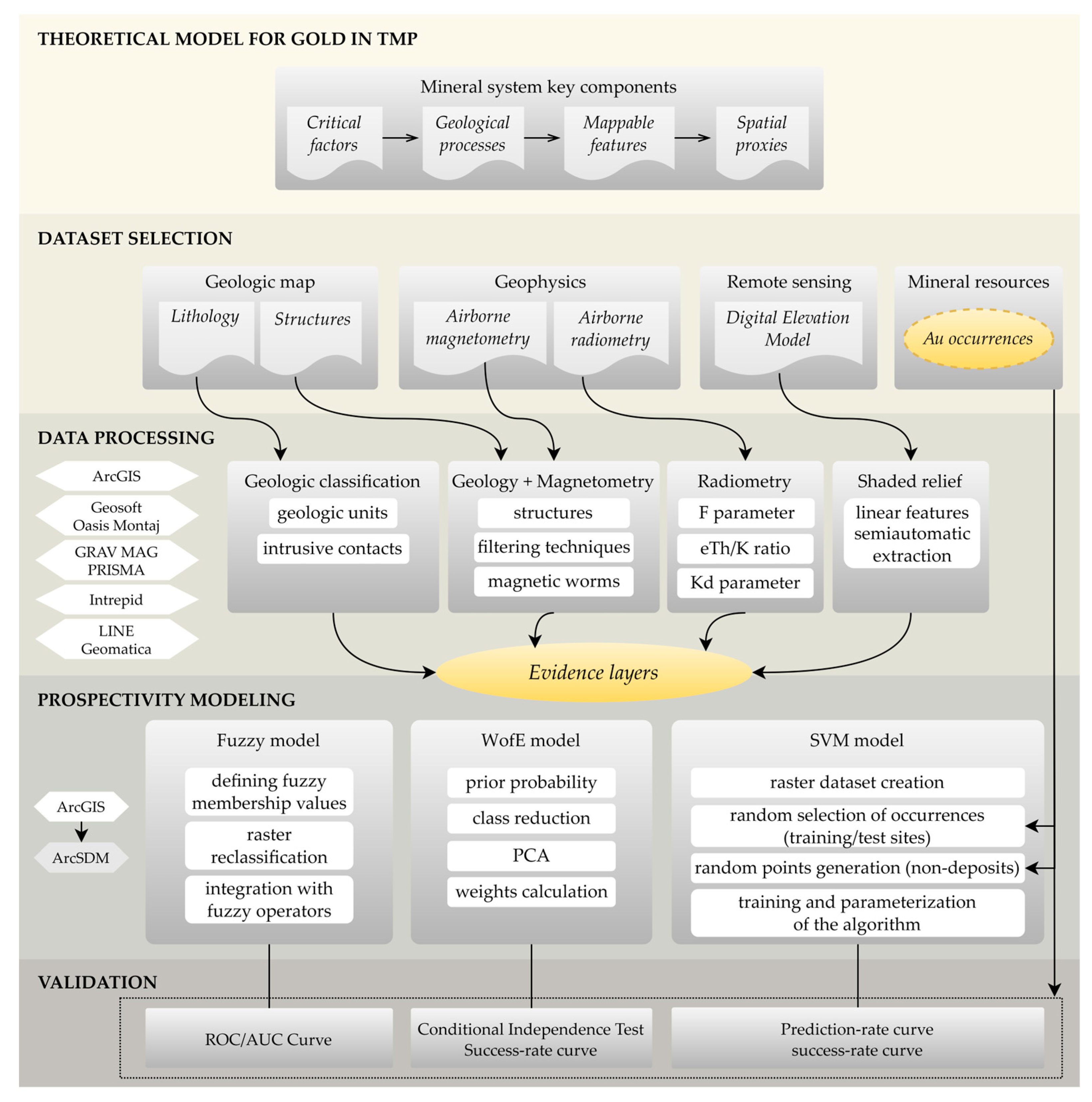
Figure 4.
Geometric and magnetic parameters of synthetic prisms. Modified from [85].
Figure 4.
Geometric and magnetic parameters of synthetic prisms. Modified from [85].
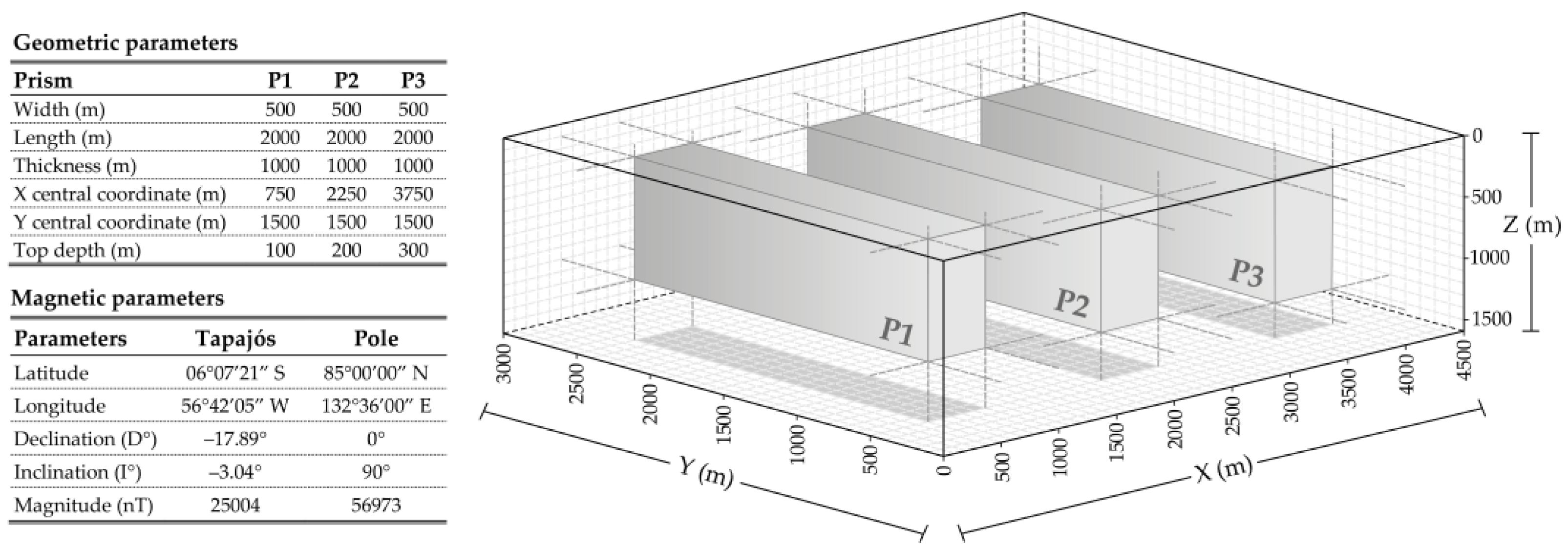
Figure 5.
Map of radiometric domains, generated from analysis of K/eTh/eU ternary image, K/eTh/eU content class map, and the geologic map. The white areas in the map correspond to the main rivers and recent sedimentary coverage, which were excluded from the analysis.
Figure 5.
Map of radiometric domains, generated from analysis of K/eTh/eU ternary image, K/eTh/eU content class map, and the geologic map. The white areas in the map correspond to the main rivers and recent sedimentary coverage, which were excluded from the analysis.
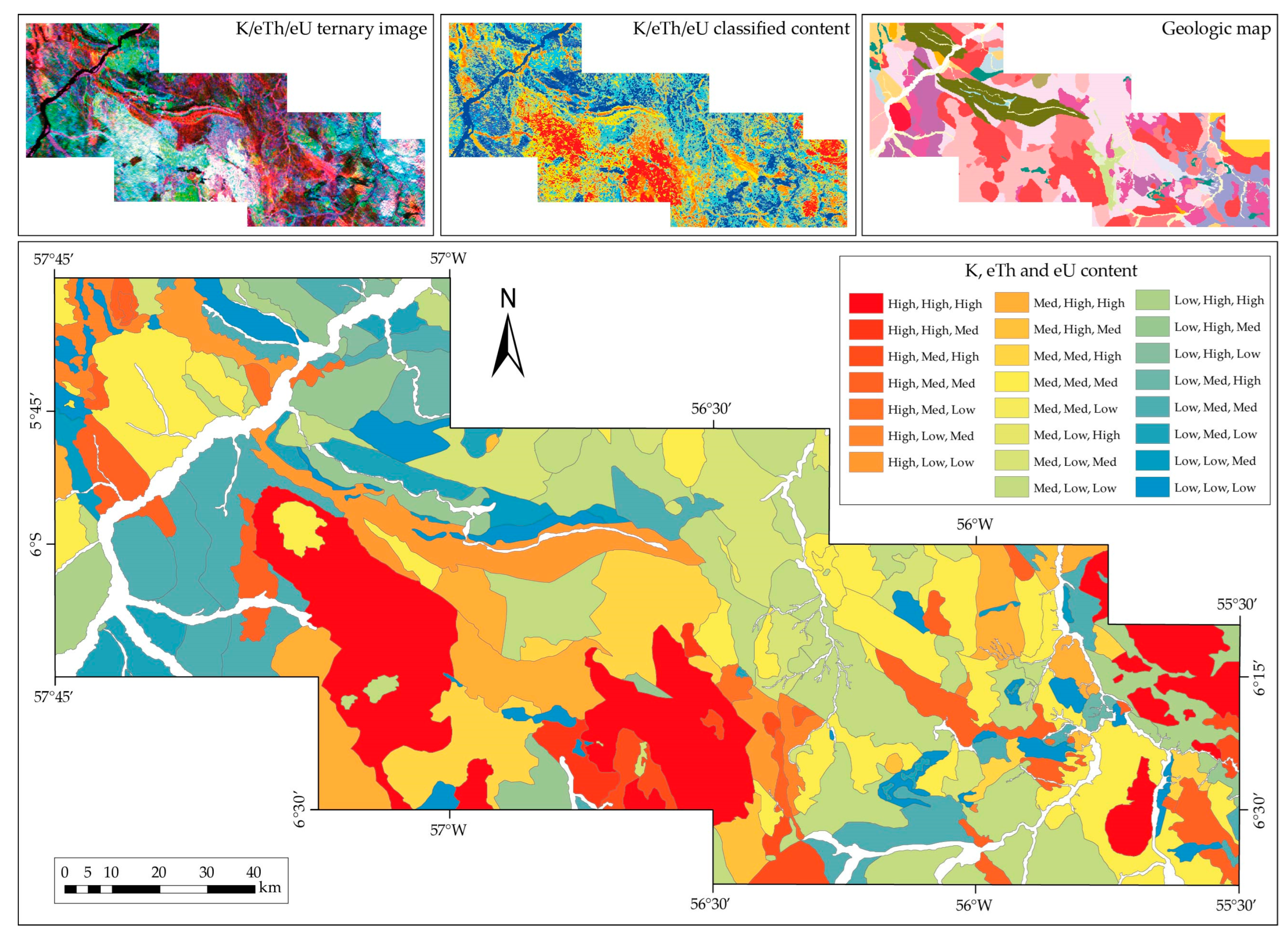
Figure 6.
Integrated maps of the (a) F, (b) Kd, and (c) Ud parameters, (d) inverted eTh/K ratio, and (e) F-Kd-eTh/K ternary composition map.
Figure 6.
Integrated maps of the (a) F, (b) Kd, and (c) Ud parameters, (d) inverted eTh/K ratio, and (e) F-Kd-eTh/K ternary composition map.

Figure 7.
Synthetic prisms and application of magnetic data enhancement filters. (a) the anomalous magnetic field and its (b) reduced–to–pole and (c) in the pole maps. (d) analytic signal amplitude and its (e) reduced–to–pole and (f) in the pole maps. (g) total horizontal gradient and its (h) reduced–to–pole and (i) in the pole maps. (j) tilt angle and its (k) reduced–to–pole and (l) in the pole maps. (m) tilt angle of the total horizontal gradient, and its (n) reduced–to–pole and (o) in the pole maps. Reduced to the pole TDR and TAHG maps are the ones that most resemble their respective maps at the pole.

Figure 8.
Parts (a–f): enhancement products applied on the 1000 m upward continuation of the AMF map reduce to pole. (g) Lineament interpretation map with the TDR-THDR map in the background. The feature frequency diagram is highlighted. n. = number of lineaments; av. dir = average direction; max. freq. = maximum frequency; conf. = confidence.
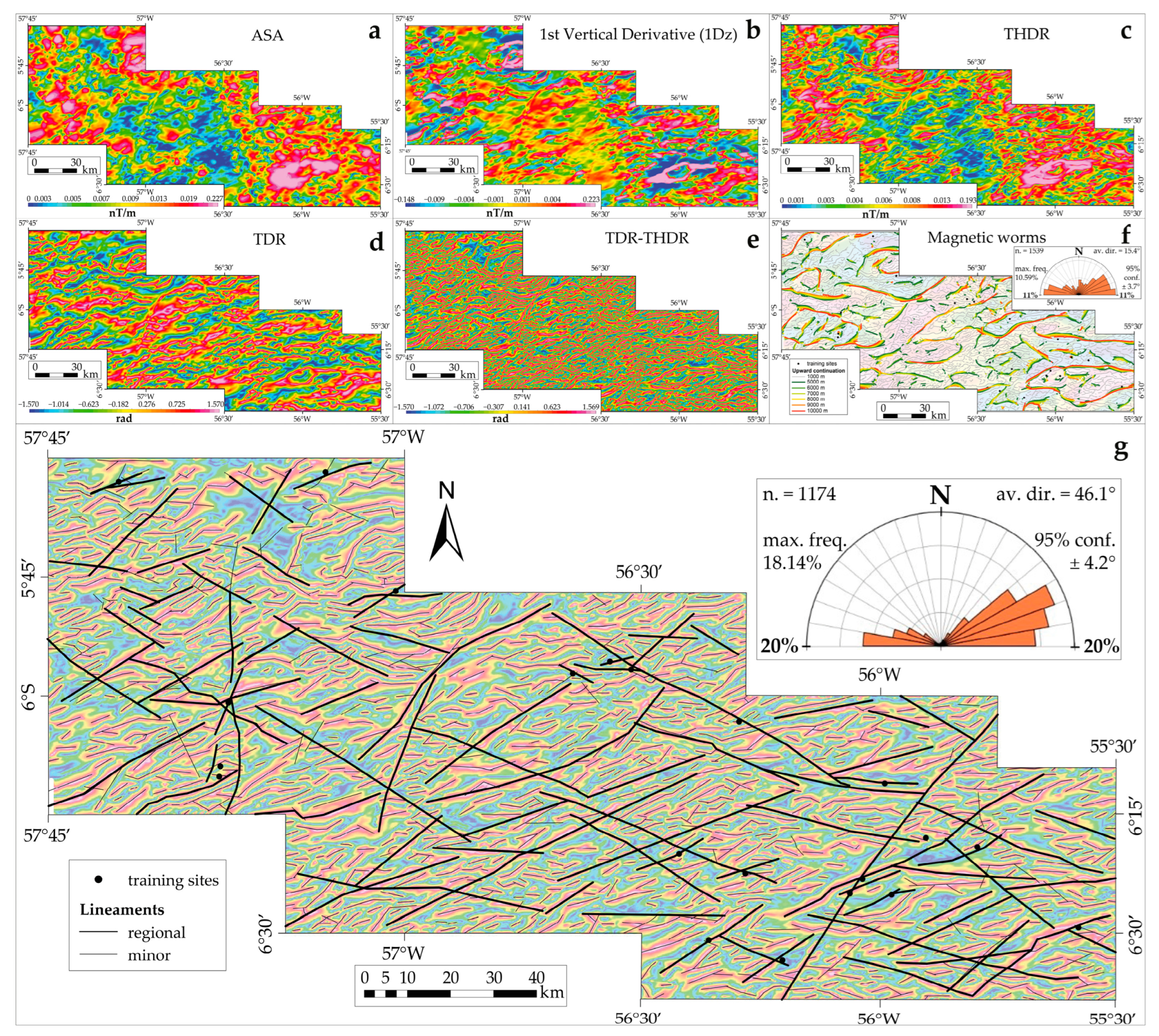
Figure 9.
(a) Multidirectional shaded relief generated with superimposing shaded reliefs on 0°, 45°, 90°, and 135° azimuths of the DEM, and (b) lineaments extracted with the LINE algorithm after correction of spurious features. The respective frequency diagram (on the right).
Figure 9.
(a) Multidirectional shaded relief generated with superimposing shaded reliefs on 0°, 45°, 90°, and 135° azimuths of the DEM, and (b) lineaments extracted with the LINE algorithm after correction of spurious features. The respective frequency diagram (on the right).
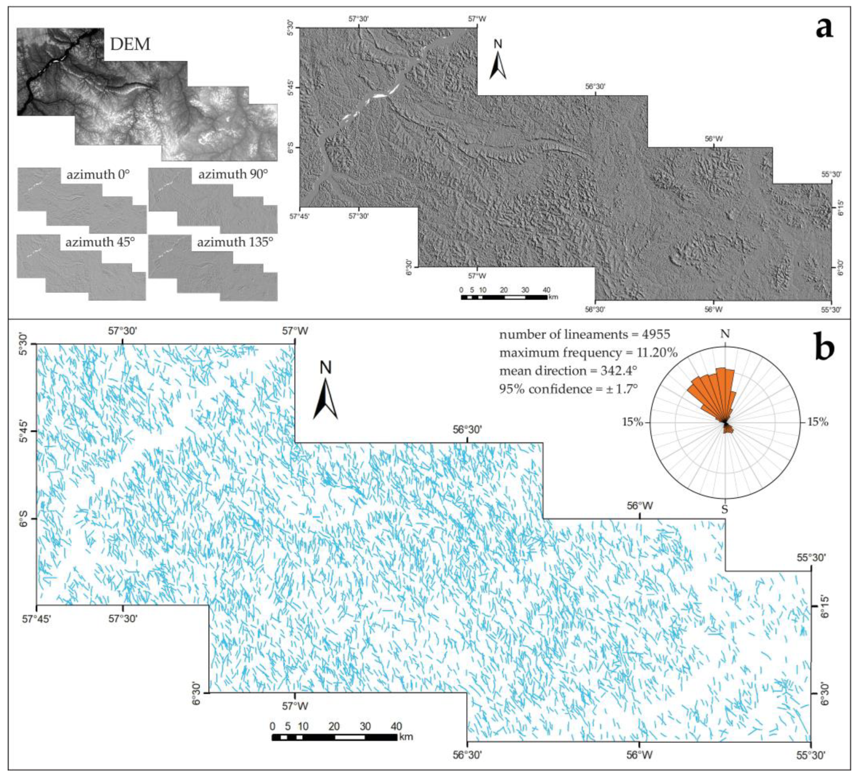
Figure 10.
Fuzzy prospectivity model for gold deposits in the central portion of the TMP. The map shows good spatial relationship between deposits and high scores of prospectivity.
Figure 10.
Fuzzy prospectivity model for gold deposits in the central portion of the TMP. The map shows good spatial relationship between deposits and high scores of prospectivity.

Figure 11.
Weights of evidence prospectivity model for the studied area.
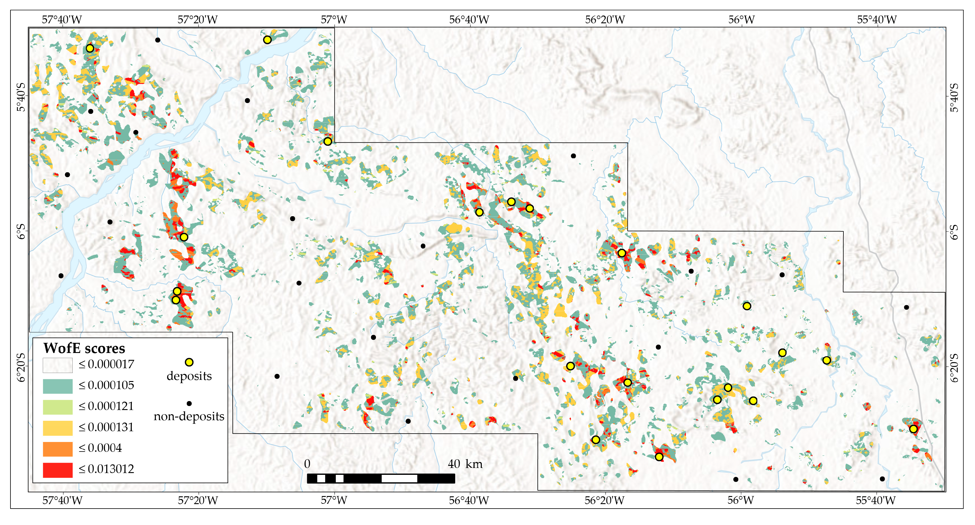
Figure 12.
SVM prospectivity model, where the values represent the distance from the hyperplane.

Figure 13.
Validation graphs: (a) ROC/AUC curve of fuzzy model; (b) ROC/AUC, prediction– and success–rates of WofE model; and (c) ROC/AUC, prediction– and success–rates of SVM model. The light blue areas in the ROC graphs correspond to the area under the curve.
Figure 13.
Validation graphs: (a) ROC/AUC curve of fuzzy model; (b) ROC/AUC, prediction– and success–rates of WofE model; and (c) ROC/AUC, prediction– and success–rates of SVM model. The light blue areas in the ROC graphs correspond to the area under the curve.

Figure 14.
Agreement map between fuzzy, WofE, and SVM models, showing 5% of the main prospective areas. Rectangles highlight areas (a) in western, (b) central, and (c) eastern sectors.
Figure 14.
Agreement map between fuzzy, WofE, and SVM models, showing 5% of the main prospective areas. Rectangles highlight areas (a) in western, (b) central, and (c) eastern sectors.
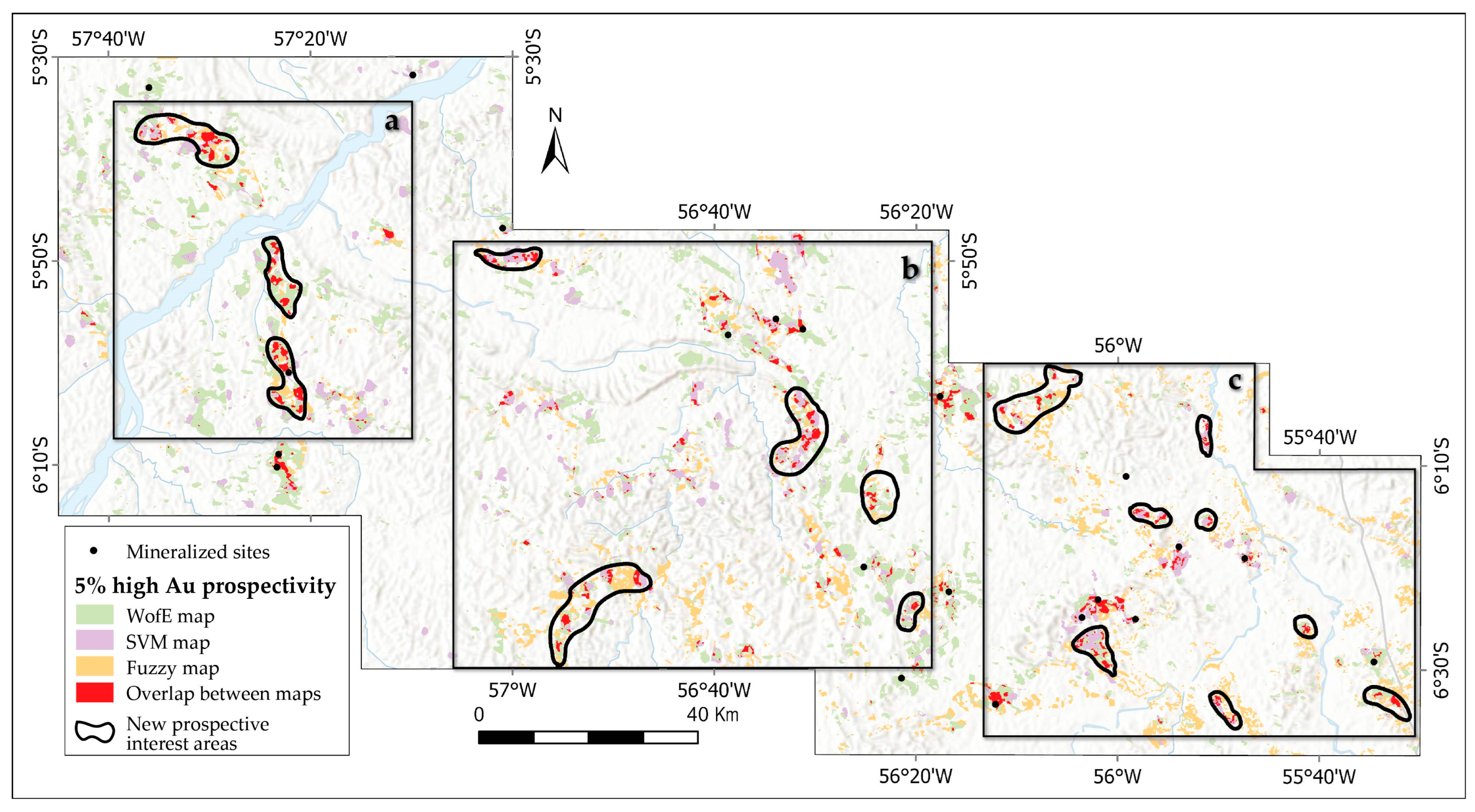

Table 1.
Data summary for the main gold prospects in the central portion of the TMP.
| Occurrence | Mineralization Style | Alteration | Structural Control | References |
|---|---|---|---|---|
| Abacate | qz veins | sil, tur | N80E/70SE | [32] |
| Água Branca | qz veins | sil, carb, sulf, ser, cl | 88/125, 35/290, 65/315 | [58,59] |
| Asa Branca | qz veins | sulf, epid | 88/175, 88/125 | [14,58] |
| Batalha | stockwork, qz veins | ser, potas, alb, epid, sil, cl | 70/315, 90/300 | [32,60,61] |
| Boa Esperança | qz veins | arg, ser, cl, sulf | 220/75SW, 80/80SE | [14] |
| Cantagalo | qz veins, stockwork, disseminations | sulf, lim, sil, kaol, arg, ser | 85/060, 90/055, 80/350 | [32,34,62] |
| Cuiú–Cuiú/Central | qz veins, hydrothermal breccia | ser, cl, carb | 75/075 | [58,63] |
| Cuiú–Cuiú/Moreira Gomes | stockwork, veins | ser, sulf, carb, cl, sil, epid | 31/305, 10/341 | [64,65] |
| Carneirinho | stockwork | sulf, sil, ser, epid, potas | N80W/85NE, N15/85SE | [14,62] |
| Davi | qz veins | ser, carb, sulf, epid, cl, potas | 90/135, 90/305 | [32,62] |
| Mamoal | mafic dykes disseminations | sulf, potas | 88/020 | [58,62] |
| Ouro Roxo | disseminations, py and qz-py veins | ser, cl, carb | 65/090, 35/095 | [32,34,66] |
| Palito | veins | ser, sulf, epid, cl, carb, potas | 88/045 | [58] |
| Pimenteiras | veins | sulf | 90/095 | [34] |
| São Chico | veins | ser, cl, sulf, epid, musc, kaol, sil | 50/170, 88/170 | [58] |
| São Domingos/Fofoca | qz-sulphide veins, stockwork | ser, sil, sulf, epid | 88/165, 72/320 | [58,67] |
| São Domingos/Tucano | stockwork, qz-sulphide veins | ser, sil, sulf, epid | 60/75NW | [58,68] |
| São João | qz veins | epid, arg, sulf | N45–65E, N30E/75SE | [37] |
| São Jorge | qz veins, stockwork disseminations | sulf, musc, cl, carb | 80/160 | [58,69] |
| Sucuba | qz veins | sil, cl | EW | [37] |
| Tocantinzinho | qz veins, stockwork | mic, cl, ser, sil, carb | 80/125, 80/345 | [58,70] |
py = pyrite; qz = quartz; sph = sphalerite; alb = albitization; arg = argilization; carb = carbonation; cl = chloritization; epid = epidotization; kaol = kaolinization; lim = limonitization; mic = microclinization; musc = muscovitization; potas = potassification; ser = sericitization; sil = silicification; sulf = sulfidation; tur = tourmalization.
Table 2.
Classification parameters for gamma-ray spectrometric channel concentrations.
| Parameters | K (%) | eTh (ppm) | eU (ppm) | |
|---|---|---|---|---|
| Mean (M) | 0.324491 | 19.620647 | 2.358534 | |
| Standard Deviation (σ) | 0.166002 | 10.636025 | 0.932671 | |
| Class | Interval | |||
| Low | <M − ½σ | <0.24 | <14.30 | <1.89 |
| Intermediate | >M − ½σ and <M + ½σ | 0.24–0.41 | 14.30–24.94 | 1.89–2.83 |
| High | >M + ½σ | >0.41 | >24.94 | >2.83 |
Table 3.
Summary of parameters used in the fuzzy logic spatial modeling process.
| Data Source | Evidence Map | Classifying Process | Prospective Thresholds | Fuzzy Operators | Integrative Operator |
|---|---|---|---|---|---|
| Geologic map, scale 1:100,000 | Favorable host rocks | Data classified according to the frequency of occurrences and geochemical signature. | - | - | GAMMA, index 0.75 |
| Geologic map, scale 1:100,000 | Intrusive contacts | Proximity analysis of deposits with the contacts of intrusive bodies. | 5000 m | - | |
| Airborne magnetometry | Magnetic lineaments | Proximity to lineaments interpreted from magnetometry, which represent the magnetic signature of mineralized shear zones, secondary deposit controls, and mineralized late veins. Euclidean distance. | 2000 m (NW) 1000 m (NE and EW) 2500 m (NS) | OR | |
| Radar image | Density of surface traces | Density of lineaments extracted from DEM. | Densities > 1 | ||
| Airborne radiometry | F parameter | Statistical classification of the values of parameters F, Kd, and Ud and the eTh/K ratio, which represent the signature of The hydrothermal alteration with positive a correlation with mineralization. | Values > M + 1σ | GAMMA, index 0.75 | |
| Kd parameter | Values > M + 1σ | ||||
| Ud parameter | Values < M − ½σ | ||||
| eTh/K ratio | Values < 0.7 |
Table 4.
PCA eigenvector matrix over the radiometric parameters. The values highlighted in blue indicate the evidence map with the greatest contribution in each PC.
Table 4.
PCA eigenvector matrix over the radiometric parameters. The values highlighted in blue indicate the evidence map with the greatest contribution in each PC.
| PC1 | PC2 | PC3 | PC4 | |
|---|---|---|---|---|
| F | 0.34639 | −0.89043 | 0.29401 | 0.02670 |
| Kd | 0.20787 | −0.17201 | −0.70639 | −0.65438 |
| Ud | 0.17715 | −0.11325 | −0.62031 | 0.75565 |
| eTh/K | 0.89745 | 0.40587 | 0.17258 | −0.00790 |
Table 5.
Comparison between the integration methods used in this work.
| Fuzzy | WofE | SVM | |
|---|---|---|---|
| Advantages | (1) Easy implementation and operator knowledge-based control. | (1) Allows analysis of the weight of each evidence map and selection of the best ones for integration. | (1) Greater robustness, and handles both linear and non-linear data; (2) generalization ability, even with few training and testing points; (3) effective separation of data with a maximum margin; (4) increases decision-making resolution. |
| Disadvantages | (1) Less precise propositions and data inputs being more susceptible to bias; (2) Many steps and parameters to define (e.g., membership functions, data classification rules, integration operators). | (1) Need to reduce the number of classes (reclassification of evidential maps); (2) the assumption of conditional independence burdened and invalidated the modeling numerous times, a problem which can be minimized with the use of PCA. | (1) Requires extensive knowledge of ML architectures and programming languages. |
Disclaimer/Publisher’s Note: The statements, opinions and data contained in all publications are solely those of the individual author(s) and contributor(s) and not of MDPI and/or the editor(s). MDPI and/or the editor(s) disclaim responsibility for any injury to people or property resulting from any ideas, methods, instructions or products referred to in the content. |
© 2023 by the authors. Licensee MDPI, Basel, Switzerland. This article is an open access article distributed under the terms and conditions of the Creative Commons Attribution (CC BY) license (https://creativecommons.org/licenses/by/4.0/).
Share and Cite
MDPI and ACS Style
Souza Gaia, S.M.d.; Souza Filho, C.R.d. Predictive Mapping of Prospectivity for Gold in the Central Portion of the Tapajós Mineral Province, Brazil. Minerals 2023, 13, 1432. https://doi.org/10.3390/min13111432
AMA Style
Souza Gaia SMd, Souza Filho CRd. Predictive Mapping of Prospectivity for Gold in the Central Portion of the Tapajós Mineral Province, Brazil. Minerals. 2023; 13(11):1432. https://doi.org/10.3390/min13111432
Chicago/Turabian StyleSouza Gaia, Sulsiene Machado de, and Carlos Roberto de Souza Filho. 2023. "Predictive Mapping of Prospectivity for Gold in the Central Portion of the Tapajós Mineral Province, Brazil" Minerals 13, no. 11: 1432. https://doi.org/10.3390/min13111432
Note that from the first issue of 2016, this journal uses article numbers instead of page numbers. See further details here.