
Application of Stacking Ensemble Learning in Predicting Copper’s Flotation Concentrate Grade
1
School of Minerals Processing and Bioengineering, Central South University, Changsha 410083, China
2
Key Laboratory of Hunan Province for Clean and Efficient Utilization of Strategic Calcium-Containing Mineral Resources, Central South University, Changsha 410083, China
*
Author to whom correspondence should be addressed.
Minerals 2024, 14(4), 424; https://doi.org/10.3390/min14040424
Submission received: 6 March 2024
/
Revised: 13 April 2024
/
Accepted: 18 April 2024
/
Published: 19 April 2024
(This article belongs to the Section Mineral Processing and Extractive Metallurgy)
Abstract
:Addressing issues such as a low operational condition recognition efficiency, strong subjectivity, and significant fluctuations in Outotec X fluorescence analysis data in copper flotation production, a copper concentrate grade classification model is constructed based on image processing technology and the Stacking ensemble learning algorithm. Firstly, a feature extraction model for copper concentration flotation foam images is established, extracting color, texture, and size statistical features to build a feature dataset. Secondly, to avoid redundancy in the feature data, which could reduce model accuracy, a combined correlation feature selection is employed for dimensionality reduction, with the filtered feature subset being used as the model input. Finally, to fully leverage the strengths of each model, a Stacking ensemble learning copper concentrate grade classification model is constructed with support vector machine (SVM), random forest (RF), and adaptive boosting (AdaBoost) as base models and logistic regression (LR) as the meta-model. The experimental results show that this ensemble model achieves good recognition for different grade categories, with a precision, recall, and F1 score of 90.01%, 89.85%, and 89.93%, respectively. The accuracy of this Stacking ensemble model, with a 7% improvement over Outotec X fluorescence analysis, demonstrates a potential to meet the daily production needs of beneficiation plants.
1. Introduction
In recent years, the sustained growth of China’s economy has significantly boosted the demand for copper, further consolidating its leading position in the global copper consumption market [1]. However, numerous challenges are faced by China in the development and utilization of copper resources, including the ubiquity of low-grade deposits, the limited reserves of high-grade ores, and the relatively lagging technological and scale development [2]. Froth flotation, a mineral processing method based on the differences in the physical–chemical properties of mineral surfaces to separate fine-grained associated or mixed minerals, has always played a crucial role in the separation and recovery of copper ores [3]. In practice, due to the complexity of the flotation process, the variety of influencing factors, and their high interdependence, the majority of beneficiation plants still rely on experienced workers to judge the grade of concentrate by observing the shape, color, and texture of the foam. This experience-based operation has drawbacks such as strong subjectivity, low identification efficiency, and difficulties standardizing evaluation criteria [4,5]. To improve this situation, some beneficiation plants have begun using X-ray fluorescence analyzers to measure the grade of concentrates, but the accuracy of this method is inevitably affected by factors such as the particle size and moisture content [6]. Therefore, researching and developing rapid, intelligent, and automated grade detection methods is of great significance for optimizing flotation process control and improving product quality.
With the rapid advancement of computer vision and machine learning, their applications in the flotation field are increasingly widespread [7,8,9]. Foam image classification and condition recognition have become hot topics in university and corporate R&D. Research on modeling to predict indicators in the flotation process primarily falls into two categories: traditional machine learning methods and deep learning. For example, Ren et al. [10] applied the least squares support vector regression (LS-SVR) model, utilizing color features of microscopic images to estimate the grade of copper concentrates. Tang et al. [11] developed a BP neural network model based on the characteristics of coal slime flotation foam images for predicting the ash content of flotation concentrates. The model integrates features like the grayscale value, quantity of foam, and average foam diameter, showing that the model’s mean relative error (MRE) is only 2.34%. In addition, researchers have used features such as foam stability and collapse rate, combined with algorithms like k-means clustering, random forests, and decision trees, to predict indicators of the flotation process [12,13]. Compared to conventional machine learning approaches, deep learning offers advantages in autonomously discovering and capturing high-dimensional abstract data features [14]. For instance, Wang et al. [15] proposed a condition recognition strategy based on image sequences, achieving an 89% accuracy rate in classifying conditions in antimony flotation tanks. Zarie et al. [16] employed a convolutional neural network (CNN) to classify flotation foam images under four different conditions, with an accuracy rate of 93.1%. Bao et al. [17] used transfer learning with Inception V1 and ResNet networks for modeling three different conditions in antimony ore flotation, achieving a high accuracy rate of 95.4%.
The above studies demonstrated how researchers utilized flotation images or foam characteristics to construct prediction models based on single algorithms. However, in practical flotation indicator predictions, multiple hypotheses might perform similarly on training sets, leading to potential randomness affecting single-model predictions, which could decrease a model’s credibility and reduce its generalization capabilities. Ensemble learning can compensate for the shortcomings of single models by integrating multiple independent models, thereby reducing errors caused by insufficient hypotheses or data randomness [18]. For example, Wang et al. [19] employed Stacking ensemble learning to construct a soil moisture content model, achieving a coefficient of determination (R2) of 0.963, which represents an improvement of 0.022 to 0.03 compared to single models. Similarly, Tang et al. [20] utilized a Stacking ensemble learning model to predict NOx emission concentrations from coal-fired boilers, demonstrating superior performance over single models. In Stacking ensemble learning, two hierarchical levels of models are employed: the first level consists of multiple base models, which are trained independently on the original dataset to capture diverse features and patterns. The second level comprises a meta-model, which utilizes the predictions of the first-level base models as input features for further training. This hierarchical approach contributes to enhancing the predictive accuracy of the model [21]. Additionally, ensemble learning has been extensively applied in diverse research fields, including photovoltaic power generation forecasts [22], rock burst predictions [23], and predictions of energy systems’ supply and demand [24].
In summary, ensemble learning, by integrating the results of multiple models, can significantly enhance the generalization ability compared to single models and achieve higher prediction accuracy. Nevertheless, the application of ensemble learning algorithms for predicting flotation process indicators remains underexplored, with most studies still favoring single-algorithm predictions. Addressing this gap, the present work, grounded in single-algorithm modeling research, proposes a copper’s flotation concentrate grade prediction algorithm, based on Stacking ensemble learning. This approach aims to improve the prediction accuracy and generalization ability of copper concentrate grade classification. Further, the study is expected to provide a foundation and theoretical support for deeper investigations into ensemble learning applications in flotation process indicator prediction, which in turn promotes the advancement of automation and intelligence in flotation processes.
2. Dataset and Methods
2.1. Copper Concentrate Grade Classification Prediction Algorithm Process
This study develops a Stacking ensemble learning model based on foam image processing and combined correlation feature selection (IPCC-SELM) for copper concentrate grade classification prediction. Figure 1 shows the IPCC-SELM modeling process, which includes three main stages: dataset collection, flotation image processing and feature selection, and grade classification model construction.
Dataset collection: This stage involves synchronously capturing copper concentration foam images and collecting samples of overflow foam from the flotation column to establish an original dataset containing both flotation images and grade data.
Flotation image processing and feature selection: During this stage, image processing techniques are employed to extract color, texture, and size statistical features from the foam images, thereby forming a feature dataset. A combined correlation feature selection approach is then applied to filter the feature subset.
Grade classification model construction: In the final stage, the selected feature subset is utilized to build a copper concentrate grade classification model. This model, based on the Stacking ensemble algorithm, incorporates support vector machines (SVM), random forests (RF), and adaptive boosting (AdaBoost) as base models, with logistic regression (LR) serving as the meta-model, and is designed to output prediction results.
2.2. Dataset Collection
In this study, the flotation foam images and concentrate grade dataset that were used were collected from the copper concentration section of a beneficiation plant in Yunnan, China. The collection apparatus was fixed at the copper flotation column, with the camera positioned 70 cm from the foam surface, capturing video of the flotation foam at a frequency of 15 min per interval. Owing to the regular anomalies and fluctuations in the readings of the Outotec X fluorescence flow analyzer in the copper flotation section, which resulted in data distortion, this study resorted to manual sampling of the concentrate overflow foam, followed by laboratory analysis, to ascertain the actual grade of the copper concentrate. Based on operational experience at the site and the concentrate’s grade, the copper flotation foam image samples were classified into six categories: (1) ultra-high (grade ≥ 19%); (2) slightly high (19% > grade ≥ 17%); (3) normal (17% > grade ≥ 15%); (4) slightly low (15% > grade ≥ 13%); (5) low (13% > grade ≥ 11%); and (6) ultra-low (grade < 11%).
2.3. Foam Image Feature Extraction
Due to the high-dimensional characteristics of flotation foam images, directly inputting them into a classification model can lead to excessively long training times and the risk of converging to local optima. The color, texture, and size of flotation foam hold specific correlations with the grade of the concentrate: during the flotation process, operators often estimate the grade based on the intensity of the foam’s color, combined with their experience. Texture features like the roughness and wrinkling of the foam surface can indicate the adhesion condition of mineral particles, while the area of the foam influences the effectiveness of mineral particle attachment [25,26,27]. In this study, 21 color features, 10 texture features, and 4 size statistical features were extracted from copper flotation foam to model the concentrate grade. Detailed feature parameters are provided in Section 2.3.1, Section 2.3.2 and Section 2.3.3.
2.3.1. Color Features
Color features are among the most intuitive visual characteristics of flotation foam, offering significant stability and robustness. In the field of image processing, RGB (red, green, blue) and HSV (hue, saturation, value) are two primary color space models. In this study, both the RGB and HSV color models are employed to extract color features from flotation foam images. Specifically, 21 color features are extracted, encompassing the mean, variance (var), and skewness (ske) of six color components—red (r), green (g), blue (b), hue (h), saturation (s), and value (v), as well as the relative mean (rel) of red, green, and blue. The mean components of color reflect the average light intensity level across various color channels. Variance measures the fluctuation and distribution range of the color intensity. Skewness describes the asymmetry of color distribution, indicating the degree and direction of deviations in color values’ distribution. Relative components are calculated by assessing the deviation of each color channel’s intensity relative to the overall mean grayscale value of the image. The formulas for calculating the aforementioned color features are as follows:
In the formulas, represents the intensity of the pixel value at position in the foam image for a specific color component. and denote the resolution dimensions of the image, and represents the overall mean grayscale value of the image.
2.3.2. Texture Features
Texture features, which quantify the statistical data of an image, represent their overall distribution and are used to describe surface characteristics such as smoothness, wrinkling, and patterns of lines. Currently, the gray-level co-occurrence matrix (GLCM) and color co-occurrence matrix (CCM) are widely utilized for their second-order statistical measures when representing texture features. This study constructs GLCMs in four orientations: 0°, 45°, 90°, and 135°. Additionally, based on the HSV color space, three CCMs are generated: CCMH,S, CCMH,V, and CCMS,V. Subsequently, using these two types of co-occurrence matrices, the study calculates the mean values of various texture features: angular second moment (Asm), entropy (Ent), contrast (Con), inverse differential moment (Idm), and texture complexity (T), resulting in a total of 10 texture features. Asm reflects the coarseness or fineness of the image texture, Ent measures the randomness, Idm indicates the uniformity of local texture, and Con assesses the level of contrast in texture. The formulas for calculating these texture features are as follows:
In the formulas, represents the co-occurrence matrix, and stands for the number of gray levels in a GLCM or quantization levels in a CCM, with a value of 8 in both cases.
2.3.3. Size Statistical Features
Extracting size statistical features from flotation foam is challenging, which is largely attributable to the foam’s irregular shapes and adhesive properties. These characteristics hinder accurate segmentation, thereby diminishing the precision of the feature extraction process. In this paper, the Otsu thresholding algorithm (Otsu) is used to segment the bright spot areas at the top of the foam. The Otsu automatically identifies the optimal threshold in the image’s grayscale histogram, dividing the image into foreground and background to either maximize or minimize inter-class variance. After the Otsu segmentation, the binarized image contains some small, spurious bright spots, necessitating additional erosion and dilation operations. Erosion helps remove these distracting bright spots, while dilation restores the overall structure of the bright spots. Figure 2 demonstrates the process of foam segmentation. The comparative analysis of the number of bright spots before and after the application of erosion and dilation shows a significant reduction in spurious bright spots. Moreover, the foam segmentation process identifies 77 bright spots, which is close to the result obtained by manual counting, demonstrating the effectiveness and accuracy of the segmentation approach.
Subsequent to the image segmentation process, the number of bright spots (the foam quantity, Fq) and the number of pixels that are occupied by these bright spots (the foam spot size, Fs) are counted. Based on these statistical measures, features such as the maximum bright spot area (Smax), the mean area of bright spots (Smean), and the mean area of foam (Fmean) can be calculated. The formulas for these calculations are as follows:
In the formula, represents the value of the pixel point located in the bright-spot-connected region of the segmented image.
2.4. Combined Correlation Feature Selection
Table 1 details a total of 35 foam features that were collected through feature extraction, organizing them from 1 to 35. However, an excessive number of features can lead to information redundancy and even interference among features, potentially compromising the accuracy of the predictive model. Consequently, selecting the most relevant features and reducing the number of feature dimensions are critical steps in developing an accurate predictive model for the concentrate grade. To achieve this, this study employs a combined correlation feature selection method for data dimensionality reduction, ensuring a balance between interpretability and predictive accuracy. Specifically, the Pearson correlation coefficient and the maximal information coefficient are used to comprehensively assess the correlation between image features and concentrate grade, thereby filtering the original feature set. The Pearson correlation coefficient quantifies the linear correlation between features and the target variable. Meanwhile, the maximal information coefficient focuses on both linear and nonlinear relationships, effectively capturing complex feature associations by measuring the maximum shared information between variables.
Figure 3 shows the Pearson correlation matrix between copper concentrate’s grade and image features. Among the color features, the correlation coefficients (R) of b_var, g_var, r_var, s_var, v_var, and s_ske with copper concentrate grade exceed 0.4. Notably, significant positive correlation (R > 0.98) is observed both among b_var, g_var, r_var, and v_var and between s_var and s_ske, indicating a partial information overlap in these groups of features. This emphasizes the necessity of reducing information redundancy in the model construction process. In terms of texture features, Asm_G, Con_G, Ent_G, Idm_G, and T_G show strong correlation with the copper concentrate’s grade (|R| > 0.53). Idm_G exhibits the strongest negative correlation (R = −0.71) with the grade, suggesting an increase in texture uniformity in samples with higher grades as the copper concentrate grade increases. Furthermore, substantial correlation exists among these texture features, with Ent_G and T_G displaying the highest correlation coefficient (R = 0.99). Regarding size statistical features, Fq, Smean, and Fmean exhibit strong correlations with the copper concentrate’s grade (|R| > 0.7), with Fmean showing the strongest negative correlation (R = −0.73), implying a decrease in the mean area of foam as the concentrate grade increases. The correlation between Smax and the concentrate grade (R = 0.22) is significantly lower than those of the other three size statistical features, indicating that the disruption or merging of flotation foam due to external interference is relatively random overall. Consequently, relying solely on the size of the top bright spots is insufficient to accurately reflect the actual state of the flotation foam. Additionally, a significant negative correlation exists between Fq and both Smean and Fmean (|R| > 0.89).
Figure 4 presents the statistical results of the maximum correlation coefficients between the concentrate grade and image features. From all the features, those with an absolute correlation coefficient (R) greater than 0.9 are selected for combination, and the remaining features are grouped separately. Then, the features with the highest maximal information coefficient or greater than 0.2 are chosen from each group. Table 2 shows the results of feature selection, and the final selected feature subset includes v_mean, b_rel, g_rel, r_rel, b_var, b_ske, s_ske, Asm_G, Idm_G, Asm_C, Idm_C, Fq, Smean, and Fmean.
2.5. Grade Prediction Based on Stacking Ensemble Learning
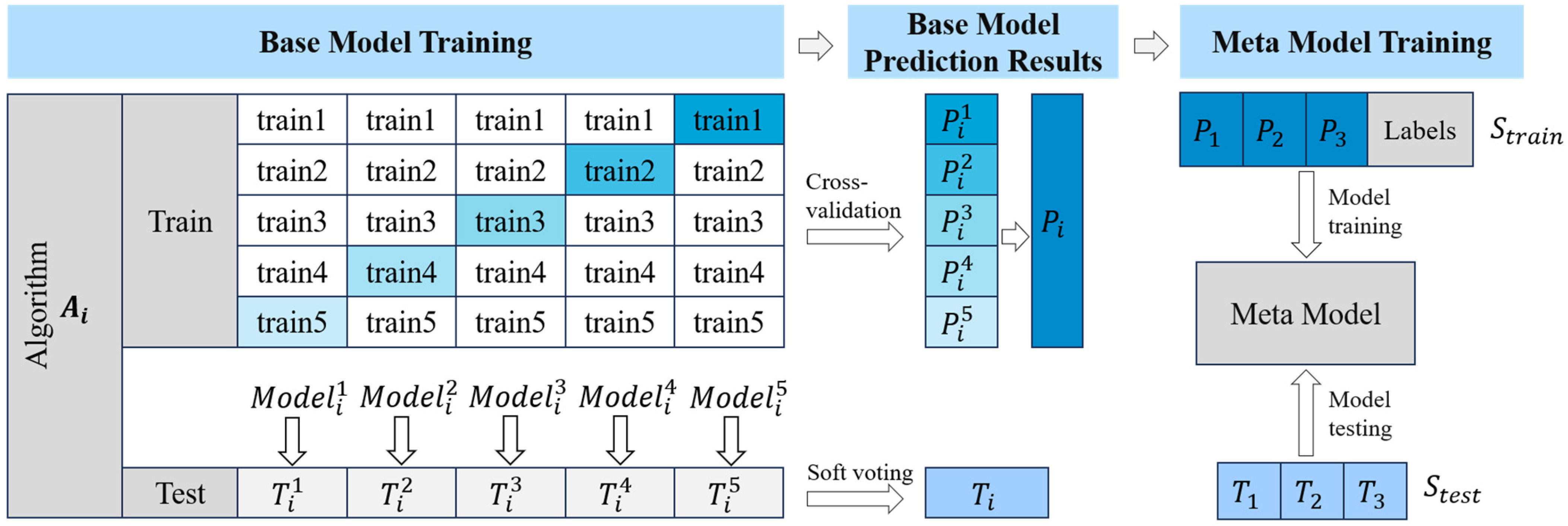
Stacking ensemble learning is a machine learning method that integrates the prediction results of multiple different base models to train a meta-model, aiming to achieve more accurate prediction outcomes [18]. This method typically consists of two layers: the first layer is composed of various base models, each making independent predictions on the same dataset; the second layer trains a meta-model based on the predictions from the first layer, thereby enhancing the model’s generalization ability and accuracy. The proposed IPCC-SELM model in this paper integrates the SVM, RF, and AdaBoost models in the first layer and employs LR as the meta-model in the second layer for final decision output. To effectively avoid the risk of model overfitting, a 5-fold cross-validation method is used to train each base model. Figure 5 illustrates the model training process.
During the Stacking ensemble learning process, the dataset, subsequent to feature selection, undergoes partitioning into a training set (Train) and a test set (Test). The training set is further segmented into five distinct, non-overlapping subsets. In each iteration of training, a combination of four subsets is selected to act as the new training data, while the fifth subset is utilized as the validation set. This cross-validation approach, which is iteratively repeated five times, ensures that each base model within the ensemble is exposed to diverse training–validation set combinations. Consequently, for each base model and in every iteration of the training phase, the developed model is formulated as follows:
In this formula, represents the model trained by the -th algorithm during the -th cross-validation, using the training set while excluding the validation subset . Here, [1, 3] represents the three base models, and [1, 5] denotes the five iterations of cross-validation.
Subsequently, each conducts classification predictions on the validation set . The resulting predictions are collected and concatenated column-wise to form . Meanwhile, the predictions of each model on the test set are computed and aggregated into through soft voting.
Finally, and are used as the training set () and the test set () for the second layer of the Stacking model to train the meta-model and produce the final ensemble prediction results.
3. Results and Discussion
To validate the effectiveness of the constructed model, this study conducts a series of experiments based on image feature extraction and feature selection. Section 3.1 examines the impact of combined correlation feature selection on the predictive model. Section 3.2 contrasts the single-algorithm models with the Stacking ensemble learning model. In Section 3.3, the influence of base- and meta-model selection is explored. Section 3.4 assesses the generalization capabilities of the ensemble model. The experimental dataset comprises 2580 foam images and 2580 corresponding grade data collected from a copper concentration flotation column at a beneficiation plant in Yunnan Province, China, with an image resolution of 500 500. Of these 2580 sets, 1920 are allocated for model training and validation, while the remaining 660 sets form the test set, utilized to evaluate the model’s generalization capability. Each grade interval in the test set is represented by 110 samples.
The model’s performance is evaluated using a confusion matrix, precision (PRE), recall (REC), and the F1 score (F1). The confusion matrix illustrates the model’s classification accuracy across different grade intervals by showing the correspondence between predicted and actual results. Precision, an accuracy measure, is calculated as the proportion of correctly predicted positive samples (TP) out of all samples predicted as positive (TP + FP, with FP indicating that the model incorrectly determines samples which are actually negative as positive samples). A high precision implies fewer false positives in positive predictions. The precision for each grade category is calculated using the following formula:
The model’s overall precision is the average of these precision values across all grade categories:
Recall measures the model’s ability to correctly identify actual positive samples (TP + FN, with FN indicating that the model incorrectly determines samples which are actually positive as negative samples). A high recall indicates that the model successfully captures a large number of actual positives. The recall for each grade interval is calculated as follows:
The model’s overall recall is the average of the recall values for all grade categories:
The F1 score, which is the harmonic mean of precision and recall, serves as a key indicator of the model’s overall performance. The closer the F1 score is to 1, the better the model’s performance is. The formula for the F1 score is as follows:
3.1. The Influence of Feature Selection on Prediction Results
This section conducts modeling validation to confirm the effectiveness of combined correlation feature selection, using the original feature dataset and the feature subset after feature selection with three algorithms: AdaBoost, SVM, and RF. Table 3 shows the performance metrics of different models with and without feature selection processing. It is observed that for the AdaBoost, SVM, and RF models after feature selection, the PRE increases by 2.44%, 7.25%, and 3.44%, respectively; REC improves by 2.72%, 5.91%, and 3.94%, respectively; and the F1 increases by 2.58%, 6.57%, and 3.69%, respectively, compared to the models without feature selection. The experimental results demonstrate that the models employing correlation-based feature selection outperform those without it, indicating that such feature selection enhances the prediction accuracy of each model.
3.2. Comparison and Analysis of Classification Results between Single-Algorithm Models and Ensemble Learning Model
To ascertain the performance superiority of the IPCC-SELM model proposed in this study, this section conducts training and modeling of the IPCC-SELM model against three single-algorithm models: SVM, RF, and AdaBoost. The focus is on comparing their classification effects on the test set. Figure 6 displays the confusion matrices of the different models, where the horizontal axis represents the actual grade category, and the vertical axis represents the predicted grade category. The codes I, II, III, IV, V, and VI, respectively, represent the six grade categories: ultra-high, slightly high, normal, slightly low, low, and ultra-low. It is observable that the three single models and the IPCC-SELM model perform excellently in identifying samples in the ultra-high- and ultra-low-grade intervals, with the IPCC-SELM model notably misclassifying only three samples in these extreme intervals. This indicates that in flotation production, the foam features of ultra-high- or ultra-low-grade samples significantly differ from those during normal operations, which aligns with the model’s predictive classification outcomes. However, the single models have a higher misclassification rate for slightly high- and normal-grade samples, mainly due to the high similarity in foam morphology between these categories and the influence of the complex production environment in the plant, leading to less-than-ideal classification results. The SVM model exhibits a high misclassification rate in identifying slightly low-grade samples, incorrectly categorizing 40 samples as low grade, highlighting its limitations in processing samples with a high feature similarity. In terms of recognition accuracy, the SVM, RF, and AdaBoost models correctly identify 525, 547, and 531 samples, respectively, while the IPCC-SELM model accurately identifies 593 samples, with only 67 samples being misclassified. This indicates that the IPCC-SELM model has a good recognition ability across all six grade categories, with a higher correct identification rate than the other single models.
Furthermore, Table 4 displays the performance metrics, comparing the IPCC-SELM model with the single models. In terms of precision, the IPCC-SELM model outperforms the SVM, RF, and AdaBoost models in all grade categories. Regarding recall, the IPCC-SELM model outperforms the other models in the ultra-high-, slightly high-, normal-, and ultra-low-grade categories. However, the PRE of the IPCC-SELM model is 80.91% and 86.36% for the slightly low- and low-grade categories, which are, respectively, lower than that of the RF and SVM. This may be due to the significant similarity in feature expression among samples in the slightly low- and low-grade categories, making it difficult for the base models to accurately differentiate these samples. The confusion matrix in Figure 6 reveals that the SVM, RF, and AdaBoost models do indeed exhibit numerous instances of mutual misclassifications in the slightly low- and low-grade categories. Since the ensemble model relies on the predictions of base models as inputs, the poor performance of the base models in these categories with complex feature relationships may directly impact the performance of the ensemble model.
Meanwhile, it becomes evident that the IPCC-SELM model demonstrates significant improvements in overall key performance metrics. Compared to SVM, RF, and AdaBoost, the IPCC-SELM model shows an enhancement in PRE of 8.71%, 7.15%, and 9.32%, respectively. Additionally, the model boosts REC by 10.30%, 6.97%, and 9.39% and heightens the F1 by 9.51%, 7.06%, and 9.36%. In the slightly high-grade category, SVM, RF, and AdaBoost demonstrate balanced precision and recall, indicating their relative accuracy and completeness in identifying this grade. In the normal-grade category, SVM leads, with a PRE of 76.42% and a REC of 85.45%, surpassing both RF and AdaBoost in REC, thus showing stronger recognition ability. In the slightly low-grade category, RF exceeds the performance of SVM and AdaBoost, with its PRE and REC being 80.17% and 84.55%, respectively, indicating better performance in this grade. The experimental results suggest that the IPCC-SELM model, by integrating the strengths of each model, achieves superior predictive performance compared to the individual models, making the IPCC-SELM model more effective in predictions.
3.3. The Influence of Base- and Meta-Model Selection on Prediction Results
To select suitable base- and meta-models for concentrate grade classification, different base models and meta-models are used to construct Stacking ensemble models. Table 5 displays the performance metrics of the different Stacking ensemble models. It can be observed that the Stacking ensemble model constructed with RF, SVM, and AdaBoost as base models and LR as the meta-model exhibits optimal performance. Its PRE, REC, and F1 are 90.01%, 89.85%, and 89.93%, respectively, demonstrating superior predictive performance compared to the other models.
From a theoretical perspective, AdaBoost enhances performance by integrating multiple weak classifiers and adjusting sample weights in each iteration, particularly emphasizing the handling of misclassified samples. SVM, through a margin maximization strategy and kernel functions, maps data to a high-dimensional space, effectively addressing linear and nonlinear data challenges. RF, by constructing multiple decision trees and implementing a voting mechanism, efficiently processes high-dimensional data while maintaining robustness and accuracy. AdaBoost, SVM, and RF, each with strong nonlinear modeling capabilities, can fully utilize their distinct advantages in fitting complex data within the Stacking ensemble framework, collaboratively enhancing the overall classification performance. LR is both simple and effective in modeling and has excellent capability and interpretability in handling various data types. LR’s linear decision boundary and probabilistic output allow it to integrate the predictive outputs of the base models clearly and efficiently in ensemble learning. The experimental results demonstrate that the Stacking ensemble model, constructed with SVM, RF, and AdaBoost as base models and LR as the meta-model, exhibits superior predictive performance compared to other ensemble models.
3.4. Validation of the Model’s Generalization Performance
To validate the generalization ability of the IPCC-SELM, this section employs a frequency-consistent photography and sampling method to collect 200 sets of foam images and grade data from the copper concentration flotation column. Additionally, grade detection results from the Outotec X fluorescence flow analyzer in the copper flotation section of the beneficiation plant are obtained from the plant’s database to serve as a reference. Table 6 shows the predictive classification results of the IPCC-SELM model on new samples, which are compared with and analyzed against the actual concentrate grade and fluorescence analysis grade. The results demonstrate that the IPCC-SELM model outperforms the Outotec X fluorescence analysis in ultra-high-, normal-, low-, and ultra-low-grade intervals, with an overall predictive classification accuracy of 84.5%, which is a 7% improvement over fluorescence analysis. This enhancement is likely due to the high misclassification rate of Outotec X fluorescence analysis under the complex on-site environment of flotation production and the latency factors in the analysis. The experiment proves that the IPCC-SELM model possesses good generalization capability and has the potential to meet the daily production needs of the beneficiation plant.
4. Conclusions
In this study, a Stacking ensemble learning model based on image processing and combined correlation feature selection is proposed, exploring the application of Stacking ensemble learning in predicting the grade of copper flotation concentrate. The following conclusions are drawn:
- Foam image processing and correlation feature selection techniques are applied to copper flotation foam images. This approach mitigates the dimensionality issues associated with high-dimensional data and reduced redundancy among the features. The experimental results indicate that using the feature subset after feature selection for modeling enhances the model’s performance.
- The copper concentrate grade classification model based on Stacking ensemble learning effectively incorporates the strengths of each base model and meta-model to fit the feature data. This model solves the problem of weak data fitting ability and poor generalization ability, which are often caused by single-algorithm modeling. The developed IPCC-SELM model achieves a precision, recall, and F1 score of 90.01%, 89.85%, and 89.93%, respectively, outperforming other models. Compared with the RF model, which has the best overall performance among the single-algorithm models, the precision, recall, and F1 score of the IPCC-SELM model are improved by 7.15%, 6.97%, and 7.06%, respectively.
- The IPCC-SELM model effectively predicts the copper’s flotation concentrate grade intervals, demonstrating strong predictive performance and generalization capability. The overall classification ability of this IPCC-SELM model is superior to Outotec X fluorescence analysis, suggesting the model’s potential to meet the daily production needs of beneficiation plants.
Author Contributions
Conceptualization, L.O.; methodology, C.Y. and L.O.; software, C.Y.; validation, C.Y. and L.O.; investigation, C.Y. and L.O.; resources, L.O.; data curation, C.Y. and L.O.; writing—original draft preparation, C.Y. and L.O.; writing—review and editing, C.Y. and L.O.; supervision, L.O.; project administration, L.O.; funding acquisition, L.O.; All authors have read and agreed to the published version of the manuscript.
Funding
The authors acknowledge financial support from the National Natural Science Foundation of China (No. 51674291).
Data Availability Statement
The article contains original contributions to the study.
Acknowledgments
We thank the support of the Key Laboratory of Hunan Province for Clean and Efficient Utilization of Strategic Calcium-containing Mineral Resources (No. 2018TP1002).
Conflicts of Interest
The authors declare no conflicts of interest.
References
- Liu, S.; Zhang, Y.B.; Su, Z.J.; Lu, M.M.; Gu, F.Q.; Liu, J.C.; Jiang, T. Recycling the domestic copper scrap to address the China’s copper sustainability. J. Mater. Res. Technol. 2020, 9, 2846–2855. [Google Scholar] [CrossRef]
- Wang, J.B.; Ju, Y.Y.; Wang, M.X.; Li, X. Scenario analysis of the recycled copper supply in China considering the recycling efficiency rate and waste import regulations. Resour. Conserv. Recycl. 2019, 146, 580–589. [Google Scholar] [CrossRef]
- Feng, Q.C.; Yang, W.H.; Wen, S.M.; Wang, H.; Zhao, W.J.; Han, G. Flotation of copper oxide minerals: A review. Int. J. Min. Sci. Technol. 2022, 32, 1351–1364. [Google Scholar] [CrossRef]
- Aldrich, C.; Avelar, E.; Liu, X. Recent advances in flotation froth image analysis. Miner. Eng. 2022, 188, 16. [Google Scholar] [CrossRef]
- Quintanilla, P.; Neethling, S.J.; Brito-Parada, P.R. Modelling for froth flotation control: A review. Miner. Eng. 2021, 162, 19. [Google Scholar] [CrossRef]
- Desroches, D.; Bédard, L.P.; Lemieux, S.; Esbensen, K.H. Suitability of using a handheld XRF for quality control of quartz in an industrial setting. Miner. Eng. 2018, 126, 36–43. [Google Scholar] [CrossRef]
- Bergh, L.; Yianatos, J.; Ulloa, A. Supervisory control strategies evaluated on a pilot Jameson flotation cell. Control Eng. Pract. 2019, 90, 101–110. [Google Scholar] [CrossRef]
- Jahedsaravani, A.; Massinaei, M.; Marhaban, M.H. Application of Image Processing and Adaptive Neuro-fuzzy System for Estimation of the Metallurgical Parameters of a Flotation Process. Chem. Eng. Commun. 2016, 203, 1395–1402. [Google Scholar] [CrossRef]
- Jovanovic, I.; Miljanovic, I. Contemporary advanced control techniques for flotation plants with mechanical flotation cells—A review. Miner. Eng. 2015, 70, 228–249. [Google Scholar] [CrossRef]
- Ren, C.C.; Yang, J.G.; Liang, C. Estimation of copper concentrate grade based on color features and least-squares support vector regression. Physicochem. Probl. Miner. Process. 2015, 51, 163–172. [Google Scholar] [CrossRef]
- Tang, M.C.; Zhou, C.C.; Zhang, N.N.; Liu, C.; Pan, J.H.; Cao, S.S. Prediction of the Ash Content of Flotation Concentrate Based on Froth Image Processing and BP Neural Network Modeling. Int. J. Coal Prep. Util. 2021, 41, 191–202. [Google Scholar] [CrossRef]
- Zhang, J.; Tang, Z.H.; Xie, Y.F.; Ai, M.X.; Gui, W.H. Visual Perception-Based Fault Diagnosis in Froth Flotation Using Statistical Approaches. Tsinghua Sci. Technol. 2021, 26, 172–184. [Google Scholar] [CrossRef]
- Zhao, L.; Peng, T.; Xie, Y.F.; Yang, C.H.; Gui, W.H. Recognition of flooding and sinking conditions in flotation process using soft measurement of froth surface level and QTA. Chemom. Intell. Lab. Syst. 2017, 169, 45–52. [Google Scholar] [CrossRef]
- Alzubaidi, L.; Zhang, J.L.; Humaidi, A.J.; Al-Dujaili, A.; Duan, Y.; Al-Shamma, O.; Santamaría, J.; Fadhel, M.A.; Al-Amidie, M.; Farhan, L. Review of deep learning: Concepts, CNN architectures, challenges, applications, future directions. J. Big Data 2021, 8, 74. [Google Scholar] [CrossRef] [PubMed]
- Wang, X.L.; Song, C.; Yang, C.H.; Xie, Y.F. Process working condition recognition based on the fusion of morphological and pixel set features of froth for froth flotation. Miner. Eng. 2018, 128, 17–26. [Google Scholar] [CrossRef]
- Zarie, M.; Jahedsaravani, A.; Massinaei, M. Flotation froth image classification using convolutional neural networks. Miner. Eng. 2020, 155, 10. [Google Scholar] [CrossRef]
- Bao, J.; Xie, Y.F.; Liu, J.P.; Tang, C.H.; Ai, M.X. Fault condition recognition based on restored image features and deep visual features. Control Theory Appl. 2020, 37, 1207–1217. [Google Scholar]
- Nie, S.Y.; He, G.C.; Shi, Y.; Zhao, H.Y.; Wu, W.B. Research progress of flotation index prediction modeling based on data driven. Chin. J. Nonferrous Metals 2023, 33, 2330–2338. [Google Scholar]
- Wang, Z.G.; Huang, Z.Q.; He, C.L.; Cai, T.Y.; Feng, Y.Q.; Lu, N.J.; Dou, H.H. Hyperspectral inversion study of Vertisol soil moisture content based on ensemble learning. J. Agric. Resour. Environ. 2023, 40, 1426–1434. [Google Scholar]
- Tang, Z.H.; Zhu, D.Y.; Li, Y. Data Driven based Dynamic Correction Prediction Model for NOx Emission of Coal Fired Boiler. Proc. CSEE 2022, 42, 5182–5193. [Google Scholar]
- Zhou, X.; Ding, L.X.; Wang, R.Z.; Ge, Q. Research on Classifier Ensemble Algorithms. J. Wuhan Univ. (Nat. Sci. Ed.) 2015, 61, 503–508. [Google Scholar] [CrossRef]
- Khan, W.; Walker, S.; Zeiler, W. Improved solar photovoltaic energy generation forecast using deep learning-based ensemble stacking approach. Energy 2022, 240, 16. [Google Scholar] [CrossRef]
- Tang, L.Z.; Xu, Q.J. Rockburst prediction based on nine machine learning algorithms. Chin. J. Rock Mech. Eng. 2020, 39, 773–781. [Google Scholar]
- Shi, J.Q.; Zhang, J.H. Load Forecasting Based on Multi-model by Stacking Ensemble Learning. Proc. CSEE 2019, 39, 4032–4042. [Google Scholar]
- Gui, W.H.; Yang, C.H.; Xu, D.G.; Lu, M.; Xie, Y.F. Machine-vision-based Online Measuring and Controlling Technologies for Mineral Flotation—A Review. Acta Autom. Sin. 2013, 39, 1879–1888. [Google Scholar] [CrossRef]
- Massinaei, M.; Jahedsaravani, A.; Taheri, E.; Khalilpour, J. Machine vision based monitoring and analysis of a coal column flotation circuit. Powder Technol. 2019, 343, 330–341. [Google Scholar] [CrossRef]
- Mehrabi, A.; Mehrshad, N.; Massinaei, M. Machine vision based monitoring of an industrial flotation cell in an iron flotation plant. Int. J. Miner. Process. 2014, 133, 60–66. [Google Scholar] [CrossRef]
Figure 1.
IPCC-SELM modeling process.

Figure 2.
Otsu foam image segmentation. (a) Original image; (b) grayscale; (c) binarization; (d) erosion; (e) dilation; (f) boundary drawing.
Figure 2.
Otsu foam image segmentation. (a) Original image; (b) grayscale; (c) binarization; (d) erosion; (e) dilation; (f) boundary drawing.

Figure 3.
Correlation matrix between copper concentrate grade and features.

Figure 4.
Maximum information coefficient between copper concentrate grade and features.

Figure 5.
Stacking ensemble model training process.

Figure 6.
Confusion matrix results of different models.


Table 1.
Flotation foam feature parameters.
| Feature Category | Feature Parameter |
|---|---|
| Color features | 1 b_mean, 2 g_mean, 3 r_mean, 4 h_mean, 5 s_mean, 6 v_mean, 7 b_rel, 8 g_rel, 9 r_rel, 10 b_var, 11 g_var, 12 r_var, 13 h_var, 14 s_var, 15 v_var, 16 b_ske, 17 g_ske, 18 r_ske, 19 h_ske, 20 s_ske, 21 v_ske |
| Texture features | GLCM: 22 Asm_G, 23 Con_G, 24 Ent_G, 25 Idm_G, 26 T_G CCM: 27 Asm_C, 28 Con_C, 29 Ent_C, 30 Idm_C, 31 T_C |
| Size statistical features | 32 Fq, 33 Smax, 34 Smean, 35 Fmean |
Table 2.
Feature selection results.
| Number | Feature Number | Selection | Number | Feature Number | Selection |
|---|---|---|---|---|---|
| 1 | 1, 2, 3, 6 | 6 | 11 | 22 | 22 |
| 2 | 4 | - | 12 | 23, 24, 25, 26 | 25 |
| 3 | 5 | - | 13 | 27, 28, 29 | 27 |
| 4 | 7 | 7 | 14 | 30 | 30 |
| 5 | 8 | 8 | 15 | 31 | - |
| 6 | 9 | 9 | 16 | 32 | 32 |
| 7 | 10, 11, 12, 15 | 10 | 17 | 33 | - |
| 8 | 13, 19 | - | 18 | 34 | 34 |
| 9 | 14, 20 | 20 | 19 | 35 | 35 |
| 10 | 16, 17, 18, 21 | 16 | - | - | - |
Table 3.
Performance metric comparison with and without feature selection.
| Metric | AdaBoost | SVM | RF | |||
|---|---|---|---|---|---|---|
| Y | N | Y | N | Y | N | |
| PRE (%) | 80.68 | 78.24 | 81.30 | 74.05 | 82.86 | 79.42 |
| REC (%) | 80.45 | 77.73 | 79.55 | 73.64 | 82.88 | 78.94 |
| F1 (%) | 80.56 | 77.98 | 80.41 | 73.84 | 82.87 | 79.18 |
Table 4.
Performance metrics comparison between the IPCC-SELM model and base models.
| Model | Category | PRE (%) | REC (%) | F1 (%) |
|---|---|---|---|---|
| SVM | Ultra-high | 98.92 | 83.64 | 80.41 |
| Slightly high | 74.29 | 70.91 | ||
| Normal | 76.42 | 85.45 | ||
| Slightly low | 78.67 | 53.64 | ||
| Low | 63.29 | 90.91 | ||
| Ultra-low | 96.23 | 92.73 | ||
| Mean | 81.30 | 79.55 | ||
| RF | Ultra-high | 95.15 | 89.09 | 82.87 |
| Slightly high | 78.18 | 78.18 | ||
| Normal | 80.58 | 75.45 | ||
| Slightly low | 80.17 | 84.55 | ||
| Low | 75.96 | 71.82 | ||
| Ultra-low | 87.10 | 98.18 | ||
| Mean | 82.86 | 82.88 | ||
| AdaBoost | Ultra-high | 94.39 | 91.82 | 80.56 |
| Slightly high | 72.41 | 76.36 | ||
| Normal | 71.65 | 82.73 | ||
| Slightly low | 68.52 | 67.27 | ||
| Low | 79.78 | 64.55 | ||
| Ultra-low | 97.35 | 100.00 | ||
| Mean | 80.68 | 80.45 | ||
| IPCC-SELM | Ultra-high | 99.07 | 97.27 | 89.93 |
| Slightly high | 90.00 | 81.82 | ||
| Normal | 82.93 | 92.73 | ||
| Slightly low | 83.96 | 80.91 | ||
| Low | 84.07 | 86.36 | ||
| Ultra-low | 100.00 | 100.00 | ||
| Mean | 90.01 | 89.85 |
Table 5.
Performance metrics of the different Stacking ensemble models.
| Base Model | Meta-Model | PRE (%) | REC (%) | F1 (%) |
|---|---|---|---|---|
| RF SVM AdaBoost | LR | 90.01 | 89.85 | 89.93 |
| RF SVM LR | AdaBoost | 86.33 | 86.05 | 86.18 |
| RF AdaBoost LR | SVM | 83.93 | 83.79 | 83.85 |
| SVM AdaBoost LR | RF | 84.49 | 84.39 | 84.44 |
Table 6.
IPCC-SELM model generalization experiment.
| Method of Grade Acquisition | Sample | Accuracy (%) | |||||
|---|---|---|---|---|---|---|---|
| Ultra-High | Slightly High | Normal | Slightly Low | Low | Ultra-Low | ||
| Actual grade | 21 | 49 | 73 | 36 | 16 | 5 | - |
| Outotec X | 18 | 46 | 48 | 31 | 8 | 4 | 77.50 |
| IPCC-SELM | 21 | 38 | 63 | 28 | 14 | 5 | 84.50 |
Disclaimer/Publisher’s Note: The statements, opinions and data contained in all publications are solely those of the individual author(s) and contributor(s) and not of MDPI and/or the editor(s). MDPI and/or the editor(s) disclaim responsibility for any injury to people or property resulting from any ideas, methods, instructions or products referred to in the content. |
© 2024 by the authors. Licensee MDPI, Basel, Switzerland. This article is an open access article distributed under the terms and conditions of the Creative Commons Attribution (CC BY) license (https://creativecommons.org/licenses/by/4.0/).
Share and Cite
MDPI and ACS Style
Yin, C.; Ou, L. Application of Stacking Ensemble Learning in Predicting Copper’s Flotation Concentrate Grade. Minerals 2024, 14, 424. https://doi.org/10.3390/min14040424
AMA Style
Yin C, Ou L. Application of Stacking Ensemble Learning in Predicting Copper’s Flotation Concentrate Grade. Minerals. 2024; 14(4):424. https://doi.org/10.3390/min14040424
Chicago/Turabian StyleYin, Chengzhe, and Leming Ou. 2024. "Application of Stacking Ensemble Learning in Predicting Copper’s Flotation Concentrate Grade" Minerals 14, no. 4: 424. https://doi.org/10.3390/min14040424
Note that from the first issue of 2016, this journal uses article numbers instead of page numbers. See further details here.