
Mixture of Akash Distributions: Estimation, Simulation and Application
by
 , , and
Anum Shafiq
1 ,
,
Tabassum Naz Sindhu
2,
Showkat Ahmad Lone
3,
Marwa K. H. Hassan
4 and
Kamsing Nonlaopon
5,*
1
School of Mathematics and Statistics, Nanjing University of Information Science and Technology, Nanjing 210044, China
2
Department of Statistics, Quaid-i-Azam University, Islamabad 44000, Pakistan
3
Department of Basic Sciences College of Science and Theoretical Studies, Saudi Electronic University, Riyadh 11673, Saudi Arabia
4
Department of Mathematics, Faculty of Education, Ain Shams University, Cairo 11566, Egypt
5
Department of Mathematics, Faculty of Science, Khon Kaen University, Khon Kaen 40002, Thailand
*
Author to whom correspondence should be addressed.
Axioms 2022, 11(10), 516; https://doi.org/10.3390/axioms11100516
Submission received: 4 September 2022
/
Revised: 20 September 2022
/
Accepted: 21 September 2022
/
Published: 29 September 2022
(This article belongs to the Special Issue Mathematical Tools and Techniques Applicable to Probability Theory and Statistics)
Abstract
:In this paper, we propose a two-component mixture of Akash model (TC-MAM). The behavior of TC-MAM distribution has been presented graphically. Moment-based measures, including skewness, index of dispersion, kurtosis, and coefficient of variation, have been determined and hazard rate functions are presented graphically. The probability generating function, Mills ratio, characteristic function, cumulants, mean time to failure, and factorial moment generating function are all statistical aspects of the mixed model that we explore. Furthermore, we figure out the relevant parameters of the mixture model using the most suitable methods, such as least square, weighted least square, and maximum likelihood mechanisms. Findings of simulation experiments to examine behavior of these estimates are graphically presented. Finally, a set of data taken from the real world is examined in order to demonstrate the new model’s practical perspectives. All of the metrics evaluated favor the new model and the superiority of proposed distribution over mixture of Lindley, Shanker, and exponential distributions.
Keywords:
mixture model; cumulative hazard rate function; Mills ratio; quantile function; least square estimationMSC:
62-XX; 62H30; 62Exx1. Introduction
In most reliability scenarios, data are modelled using a single parametric model. However, in certain circumstances, a population can be split into many subgroups, each showing a particular category of collapse. Finite mixture models serve a significant role in modelling such diverse data. Biology, business, engineering, healthcare, genetics, marketing, real-world applications, and social sciences all benefit from finite mixture models. Mixture models are created by varying the proportions of two or more models to generate a new distribution with novel properties. Consequently, it is essential to examine the statistical characteristics of the suggested mixture model and employ the suitable methods for estimating the unexplained parameters. Mixture models are used in a diversity of applications, such as clustering and classification [1,2,3,4]. Sultan et al. [5] proposed a mix of inverse Weibull models and utilized density and hazard function graphs to study some of its features. The conventional characteristics of the concoction of Burr XII and Weibull distributions were examined by [6]. Recently, the authors [7,8], Ateya [9], Mohammadi et al. [10], and Al-Moisheer et al. [11] are among the scientists who study mixture modelling in a variety of contexts.
Many applied sciences, including medical, engineering, insurance, and finance, rely on lifetime data modelling and analysis. Some of the continuous distributions used to explain lifetime data are Weibull, gamma, exponential, lognormal, and Lindley, as well as their generalizations. Since many investigators have employed Lindley distribution to predict lifetime data, and Hussain [12] has demonstrated that Lindley model is effective for stress-strength dependability modelling, Lindley model may not be suitable for describing real-world data in many cases. Shanker [13] developed a novel model by using a two-component concoction of an exponential model and a gamma model to have a unique distribution that is more flexible than Lindley and exponential distribution for modelling lifespan data in terms of dependability and hazard rate shapes. Shanker et al. [14] have devised and addressed the concept of modelling lifetime data using one parameter families of distributions, such as Akash, exponential, and Lindley distributions. Many lifetime datasets are employed to exhibit its adaptability over the exponential distribution. Shanker and Shukla [15] examined the two-parameter Akash model and determined its statistical characteristic, estimation problem, and application to it. As a reason, the Akash distribution can be used as an alternate lifetime model in reliability analysis.
The maximal likelihood estimation (MLE) is well-known estimation approach. Despite the fact that MLE is efficient and has strong conceptual features, there is confirmation that it does not work well, especially with small samples. As a result, different estimation approaches have been offered in the studies as options to conventional method. The weighted least-squares estimation (WLSE), L-moments estimator (LME), percentile estimator (PCE) and least squares estimator (LSE) are among the most frequently recommended. These approaches, in general, do not possess desirable theoretical features, but they can offer better estimates of unknown parameters in specific instances than the MLE. Various estimating approaches for many models have been investigated in the studies, as illustrations [16,17,18,19,20,21]. The goal of this research is to give a mechanism for expert statisticians to choose the best evaluation method for the Two-Component Mixture of Akash Model (TC-MAM). In this investigation, we estimate the TC-MAM using LSE and WLSE, in conjunction to MLE.
Our goal in this investigation is to develop a novel mixture model for modeling real lifespan datasets from various disciplines of knowledge that is better fitting than mixture of Shanker, exponential and Lindley distributions. The TC-MAM model has an advantage over the Shanker and exponential models because the exponential distribution has a constant hazard rate function and the Shanker model has an increasing hazard rate function, whereas the failure rate function for a TC-MAM model exhibits monotonically increasing, modified declining, decreasing–increasing–decreasing (DID), declining–increasing (DI), and upside-down bathtub behavior. The novel TC-MAM is being developed in particular to offer a novel flexible parametric model for modeling complex data that emerges in dependability research, investigation of lifespan, quality control, statistical mechanics, economics, biological investigations, and other fields. The purpose is to provide a novel model for lifespan analysis that can handle various types of failure rates, as well as various close form features of novel model with simple physical interpretations.
The originality of this research is due to the fact that we present a thorough explanation of the statistical aspects of TC-MAM in the hopes of attracting more applications in lifespan analysis. Additionally, as far as we know, no investigation has been performed to evaluate all of these estimators of the TC-MAM, as well as their mathematical and statistical features and assessment methods to estimate of unexplained parameters of TC-MAM. For various sample sizes and parametric values, we demonstrate how alternative frequentist estimators of the suggested distribution work.
2. The Two-Component Mixture of Akash Model
A T is stated to have a TC-MAM if its PDF and CDF can be integrated as:
and
where and is a positive mixing parameter, whereas are positive scale parameters.
2.1. Mode
By tackling the given non-linear equation with respect to t, the mode of the TC-MAM() is derived
2.2. Median
The median of TC-MAM is given here. Let be CDF of TC-MAM the median is at 50th quantiles that is . The median () can, therefore, be determined by resolving given equation for t.
Numerical strategies like Newton–Raphson approach can be utilised to find from Equation (7).
Several graphs of PDF and CDF of TC-MAM, as well as both component densities, for various parametric values are shown in Figure 1 and Figure 2. It should be indicated that input parameters were selected at random until a wide range of patterns could be examined. The PDF exemplifies its adaptability. The PDF curves of TC-MAM() indicate that it can be monotonically decreasing, positively skewed, inverted U, and declining–increasing–decreasing (DID), as well as modified monotonically decreasing with platykurtic, mesokurtic, and leptokurtic curves. As a result, it can be used to model a diverse set of data.
2.3. mth Moments about Origin
For a r.v. T, the mth moments of TC-MAM are as:
The mean of the TC-MAM is:
while the variance is given by
Graphs of the mean and variance of TC-MAM () for a variety of parameter values that can be identified in Figure 3 and Figure 4. The mean of TC-MAM (), shows a monotonically decreasing behavior for fixed value of and and varying values of (see Figure 3a). The escalating changes of mixing parameter enhanced the mean concentration, according to this analysis. We draw mean graphs (see Figure 3b) to demonstrate the behavior of the mean for fixed values of and and varying values of . It reveals the characteristics of component parameter in relation to a mean profile. The boosting attitude of reduce the concentration of mean for the all varying values of . The significances of the mixing parameter versus the mean profile are defined in Figure 3c for various levels of . From these drawn lines, it can be deduced that the concentration of the mean profile is a deteriorating function for parameter . The variance exhibits the same behavior as the mean in all scenarios (see Figure 4a–c).
In particular moments about origin
and the moments about mean of the TC-MAM are:
The (Coefficient of Variation), (Skewness) and (Kurtosis) of TC-MAM are:
and Index of Dispersion is
The TC-MAM is readily explained to be over-distributed when , equi-dispersed as well as under-dispersed
Graphs of the ID of TC-MAM () for various parameter settings are illustrated in Figure 5. The boosting attitude of rise the concentration of mean for the all varying values of (see Figure 5a). However, boosting attitude of reduces the concentration of mean for the all varying values of (see Figure 5b). The effects of against the concentration of the mean profile are shown in Figure 5c. The concentration of the mean profile is a decreasing function for parameter according to these depicted lines. Figure 6 and Figure 7 explain the nature of and in relation to , and The coefficient of skewness and kurtosis of TC-MAM (), shows a decreasing behavior for fixed value of and and varying values of (see Figure 6a and Figure 7a).
To expose the behavior of and for fixed value of and and varying values of (see Figure 6b and Figure 7b). The escalating changes of mixing parameter enhanced and concentration, according to this analysis. The significances of the mixing parameter versus the coefficient of skewness and kurtosis profile are defined in Figure 6c and Figure 7c for various levels of . From these drawn lines, it can be deduced that the concentration of the skewness and kurtosis profile is a deteriorating function for parameter .
2.4. Moment Generating Function
The MGF of TC-MAM is specified as:
2.5. Cumulants
The cumulants (CF), of TC-MAM is derived by plugging with ‘’ in Equation (22), the following formula can be used to obtain the CF:
where the complex unit .
2.6. Probability Generating Function (PGF)
In Equation (22), the PGF by plugging with “ln()” is:
2.7. Factorial Moment Generating Function
By plugging with ‘ln’ in Equation (22), the FMGF can be shown as
3. Reliability Measures
In reliability framework, lifetime models are classified using the reliability/survival function and the failure/hazard rate function. TC-MAM is currently being studied for its reliability properties.
3.1. Reliability Function
The reliability function of TC-MAM is.
3.2. Hazard Function
The failure rate function of the TC-MAM() is described as follows.
In Figure 8, the HRF of TC-MAM shows monotonically increasing, modified decreasing, decreasing–increasing–decreasing (DID), decreasing–increasing (DI), and upside down bathtub behavior. Figure 8a,b,d signifies that the reduction in failure rate function profile and is noted by enlarging the value of mixing parameter and for . Figure 8c,e,f exhibits the diversion in the failure rate function for various values of . It is found in Figure 8 that the failure rate distribution is expanding due to higher the value of mixing parameter and for
3.3. Mills Ratio
Mills ratio is an another method of quantifying reliability due to its relation to failure rate. Mills ratio of TC-MAM() is
3.4. Cumulative Hazard Rate Function
The CHRF of TC-MAM is
It is a risk indicator: the stronger the estimate, the greater the chance of failure by t-time. It must be stated that
So,
3.5. Reversed Hazard Rate Function
The RHRF of a random life of TC-MAM is defined as
3.6. Mean Time to Failure (MTTF)
The expected time for which the device performs efficiently is given by the mean time to failure (MTTF). If TC-MAM then reliability function is used to express MTTF, which is as follows:
and is provided in Equation (28). Thus
4. Estimation Inference via Simulation
Given that the parametric vector is undetermined, certain statistical properties of the TC-MAM() are presented to this section. The evaluation of parametric vector is accomplished by three widely known estimation mechanisms, such as MLE, LSE, and WLSE. From now, signify n determined values from T and their ascending sorting values
4.1. Maximum Likelihood Estimation (MLE)
The MLE method is the best methodology for parameter assessment. The popularity of the approach stems from its many advantageous characteristics, such as consistency, normality, and asymptotic efficiency. Let be n determined values from the Equation (2) and be the vector of undetermined parameters. The evaluations of MLEs of can be given by optimizing the likelihood function with respect to and given by or likewise the log-likelihood function for is
So, by partially differentiating in terms of each parameter () and placing the results to zero, the MLEs of the relevant parameters are determined as
As a consequence, the MLE is found by evaluating this non-linear set of equations. However such equations cannot be handled analytically, we can use statistical software to solve them using an iterative methodology namely the Newton method or fixed point iteration methods.
4.2. Least Square Estimators (LSE)
The ordinary least square approach [22] is widely used for assessing undetermined parameters. The LSEs of and , indicated by and , can be determined by minimizing Equation (42)
with respect to and , where ·)is given by Equation(4). They may be determined in the similar way by solving the non-linear equations below:
and
where
4.3. Weighted Least Squares Estimators (WLSE)
Take a look at the following weighted function (see [23])
The WLSEs and , can be obtained by minimizing Equation (50)
One can also obtain these estimators by solving:
and
where and are given in Equations (46)–(48).
4.4. Simulation Study
The simulation study is used to evaluate the various estimating methodologies outlined in the preceding subsection. Monte Carlo simulations are performed with a variety of mixing proportion and distribution parameters. The performance of MLE, LSEs, and WLSEs of the TC-MAM() parameters is evaluated using four simulation experiments. The proficiency of the MLEs, LSEs, and WLSEs is discussed using the bias and MSE indicators. In terms of n, the efficiency of each parameter estimation strategy for the TC-MAM() model is examined. The simulation algorithm is subdivided into six steps:
- By adjusting the mixing proportion and model parameters Set-I Set-II and Set-III, generate random samples of sizes from TC-MAM(). The random samples for the simulation are obtained as specified in the upcoming stage.
- Generate a random variable u from uniform distribution , employing R uniform generator (runif).
- If , then generate a random variable from the first component, which is a Akash distribution . If , the second component, Akash distribution , is utilized to produce a random variate.
- Follow (2 and 3) till you have the prescribed sample size n.
- Employing 1000 iterations, continue steps 1–4 each time. Evaluate MLEs, LSEs, and WLSEs for the 1000 samples, say for having optima function and the Nelder–Mead technique in R to compute estimates.
- Determine biases and MSEs. The two metrics are utilized to meet these targets:where
The empirical findings are depicted in Figure 9, Figure 10, Figure 11, Figure 12, Figure 13 and Figure 14. These results suggest that the proposed estimation methods are effective at estimating the TC-MAM parameters. We can deduce that the estimators display asymptotic unbiasedness because the bias goes to zero as n rises. On the other hand, MSE behavior implies consistency because the errors trend to zero as n increases. The following conclusions can be drawn from Figure 9, Figure 10, Figure 11, Figure 12, Figure 13 and Figure 14.
- Under all three estimation procedures, the estimated bias of parameters reduces as n grows.
- The estimators of are over-estimated in the third scenario, however the over and under estimation of and are seen among the three investigated estimators, and the WLSE always has the minimum value of bias of all estimators (see Figure 13).
- Among the three estimators evaluated, the MSE of is the greatest (see Figure 14).
- The MSE of is strongly stimulated and higher under MLE and LSE estimation methods when (see Figure 10).
- Some big shifts in MSEs of considered estimators under MLE, LSE, and WLSE are observed when .
- In terms of bias, the WLSE’s performance is relatively favorable.
- In all estimating methodologies, the difference between estimates and stated parameters reduces as n rises.
- As n approaches infinity, WLSE estimation is frequently better in terms of bias and MSE when likened to other estimation methods for all given parameter values.
- The estimated MSEs of parameters and under the MLE estimation technique decrease quickly as n increases, demonstrating the effectiveness of the MLE procedure.
The final conclusion drawn from the foregoing figures is that, as n rises, estimated bias and MSE graphs for estimators , , and finally approach zero for all estimating methods. This demonstrates the accuracy of both the estimating methods and the numerical computations for the TC-MAM parameters.
5. Applications
We demonstrate the flexibility of the TC-MAM in this section by examining a real dataset. The TC-MAM distribution is compared to competing models, such as the two component mixture of Shanker distribution (2C-MSM), the two component mixture of exponential model (2-CMEM), and the two component mixture of Lindley distribution (2C-MLM) using the R function maxLik(). The -Log-likelihood (-LL), the AIC, BIC, and AICC have all been used to compare these models. The model having the least quantities of above-mentioned goodness-of-fit (GoF) measures may be the best fit for the real dataset.
Dataset: There are 56 observations in this dataset pertaining to the burning velocity of various chemical substances. The laminar flame speed at the specified composition, temperature, and pressure circumstances is the burning speed/velocity. It lowers as the inhibitor concentration rises, and it may be observed directly by analysing the pressure distribution in the spherical vessel and monitoring the flame propagation. We consider a real-life dataset which represents the burning velocity (cm/s) of several chemical compounds to show the TC-MAM distribution’s suitability. This dataset is extracted from https://www.cheresources.com/mists.pdf (accessed on 4 September 2022) and the data are as follows: 68, 61, 64, 55, 51, 68, 44, 50, 82, 60, 89, 61, 54, 166, 66, 50, 87, 48, 42, 58, 46, 67, 46, 46, 44, 48, 56, 47, 54, 47, 89, 38, 108, 46, 40, 44, 312, 41, 31, 40, 41, 40, 56, 45, 43, 46, 46, 46, 46, 52, 58, 82, 71, 48, 39, and 41 [24,25,26,27] contains further data applications. The MLEs for the TC-MAM and GoF measures are shown in Table 1. The TC-MAM clearly outperforms the 2-CMSM, 2-CMEM, and 2-CMLM, as shown in Table 1. The profiles of the log-likelihood function (PLLF) based on the dataset that confirm the conclusions of Table 1 are shown in Figure 15. Figure 15 and Figure 16 show a graphical illustration of MLE existence and uniqueness, respectively. To summarize, the TC-MAM emerges as the better model for the dataset, indicating its usefulness in a real-world setting. We can deduce from this graphical representation and results obtain from Table 1 that the TC-MAM is a better fit for the dataset in consideration.
6. Conclusions
In this investigation, we used three estimated techniques: MLE, LSE, and WLSE to work on two component mixtures of Akash models. In particular, the Akash mixing model’s statistical and reliability features were achieved, such as central moments, Cumulants, Cumulant Generating Function, Probability Generating Function, Mean Time to Failure, Factorial Moment Generating Function, Coefficient of variation, Mills ratio, skewness and kurtosis, Reversed Hazard Rate Function, and Mean Residual Life. To investigate and assess the estimating approaches’ performance, a simulation study with 1000 iterations was performed and it was noted that when n increases, the estimated MSEs of parameters and under the MLE estimation technique rapidly decrease, illustrating the efficiency of the MLE procedure. As a result, we found that estimating model unknown parameters with regards of accuracy and consistency, the MLE approach surpassed the rest. Furthermore, we used real datasets to explain the utility of the underlying mixture model.
Author Contributions
Author Contributions: Conceptualization, A.S., T.N.S. and S.A.L.; methodology, A.S., M.K.H.H. and T.N.S.; validation, S.A.L. and T.N.S.; formal analysis, A.S., T.N.S. and K.N.; investigation, M.K.H.H., T.N.S. and S.A.L.; writing—original draft preparation, A.S., T.N.S. and S.A.L.; writing—review and editing, A.S., M.K.H.H. and K.N. All authors have read and agreed to the published version of the manuscript.
Funding
This research received no external funding.
Data Availability Statement
All the data are available in this manuscript.
Conflicts of Interest
Authors declare that they do not have conflicts of interest.
Nomenclature
| Symbols | |
| Mills Ratio | |
| PGF | |
| CHRF | |
| MGF | |
| RF | |
| CGF | |
| MTTF | |
| CDF | |
| HRF | |
| QF | |
| CF | |
| FMGF | |
| RHRF | |
| MRL | |
| Abbreviations | |
| CHRF | Cumulative Hazard Rate Function |
| MGF | Moment Generating Function |
| Probability Density Function | |
| CGF | Cumulant Generating Function |
| CDF | Cumulative Distribution Function |
| FMGF | Factorial Moment Generating Function |
| RHRF | Reversed Hazard Rate Function |
| PGF | Probability Generating Function |
| WLSE | Weighted Least Square Estimator |
| MLE | Maximum likelihood Estimator |
| AICC | Akaike Information Criterion Corrected |
| AIC | Akaike Information Criterion |
| TTF | Time-To-Failure |
| QF | Quantile Function |
| RF | Reliability Function |
| CF | Characteristic Function |
| MSE | Mean square error |
| MRL | Mean Residual Life |
| LSE | Least Square Estimator |
| r.v. | Random Variable |
| HRF | Hazard Rate Function |
| MTTF | Mean Time to Failure |
| GoF | Goodness-of-Fit |
| BIC | Bayesian Information Criterion |
References
- Everitt, B.S. A finite mixture model for the clustering of mixed-mode data. Stat. Probab. Lett. 1988, 6, 305–309. [Google Scholar] [CrossRef]
- Lindsay, B.G. Mixture models: Theory, geometry and applications. In NSF-CBMS Regional Conference Series in Probability and Statistics; Institute of Mathematical Statistics: New York, NY, USA, 1995; p. i-163. Available online: https://www.jstor.org/stable/4153184 (accessed on 4 September 2022).
- McLachlan, G.J.; Basford, K.E. Mixture Models: Inference and Applications to Clustering; M. Dekker: New York, NY, USA, 1988; Volume 38. [Google Scholar]
- McLachlan, G.; Peel, D. Finite Mixture Models; John Wiley & Sons: New York, NY, USA, 2000. [Google Scholar]
- Sultan, K.S.; Ismail, M.A.; Al-Moisheer, A.S. Mixture of two inverse Weibull distributions: Properties and estimation. Comput. Stat. Data Anal. 2007, 51, 5377–5387. [Google Scholar] [CrossRef]
- Mohammad, D.; Muhammad, A. On the Mixture of BurrXII and Weibull Distribution. J. Stat. Appl. Probab. 2014, 3, 251–267. [Google Scholar]
- Sindhu, T.N.; Feroze, N.; Aslam, M.; Shafiq, A. Bayesian inference of mixture of two Rayleigh distributions: A new look. Punjab Univ. J. Math. 2020, 48, 49–64. [Google Scholar]
- Sindhu, T.N.; Hussain, Z.; Aslam, M. Parameter and reliability estimation of inverted Maxwell mixture model. J. Stat. Manag. Syst. 2019, 22, 459–493. [Google Scholar] [CrossRef]
- Ateya, S.F. Maximum likelihood estimation under a finite mixture of generalized exponential distributions based on censored data. Stat. Pap. 2014, 55, 311–325. [Google Scholar] [CrossRef]
- Mohammadi, A.; Salehi-Rad, M.R.; Wit, E.C. Using mixture of Gamma distributions for Bayesian analysis in an M/G/1 queue with optional second service. Comput. Stat. 2013, 28, 683–700. [Google Scholar] [CrossRef]
- Al-Moisheer, A.S.; Daghestani, A.F.; Sultan, K.S. Mixture of Two One-Parameter Lindley Distributions: Properties and Estimation. J. Stat. Theory Pract. 2021, 15, 11. [Google Scholar] [CrossRef]
- Hussain, E. The Non-Linear Functions of Order Statistics and Their Properties in Selected Probability Models. Ph.D. Thesis, Department of Statistics, University of Karachi, Karachi, Pakistan, 2006. [Google Scholar]
- Shanker, R. Akash distribution and its applications. Int. J. Probab. Stat. 2015, 4, 65–75. [Google Scholar]
- Shanker, R.; Hagos, F.; Sujatha, S. On modeling of lifetime data using one parameter Akash, Lindley and exponential distributions. Biom. Biostat. Int. J. 2016, 3, 1–10. [Google Scholar] [CrossRef]
- Shanker, R.; Shukla, K.K. On two-parameter Akash distribution. Biom. Biostat. Int. J. 2017, 6, 416–425. [Google Scholar] [CrossRef]
- Dey, S.; Kumar, D.; Ramos, P.L.; Louzada, F. Exponentiated Chen distribution: Properties and estimation. Commun. Stat.-Simul. Comput. 2017, 46, 8118–8139. [Google Scholar] [CrossRef]
- Dey, S.; Alzaatreh, A.; Zhang, C.; Kumar, D. A new extension of generalized exponential distribution with application to ozone data. Ozone Sci. Eng. 2017, 39, 273–285. [Google Scholar] [CrossRef]
- Rodrigues, G.C.; Louzada, F.; Ramos, P.L. Poisson exponential distribution: Different methods of estimation. J. Appl. Stat. 2018, 45, 128–144. [Google Scholar] [CrossRef]
- Dey, S.; Moala, F.A.; Kumar, D. Statistical properties and different methods of estimation of Gompertz distribution with application. J. Stat. Manag. Syst. 2018, 21, 839–876. [Google Scholar] [CrossRef]
- Dey, S.; Josmar, M.J.; Nadarajah, S. Kumaraswamy distribution: Different methods of estimation. Comput. Appl. Math. 2018, 37, 2094–2111. [Google Scholar] [CrossRef]
- Shafiq, A.; Batur Çolak, A.; Naz Sindhu, T.; Ahmad Lone, S.; Alsubie, A.; Jarad, F. Comparative study of artificial neural network versus parametric method in COVID-19 data analysis. Results Phys. 2022, 38, 105613. [Google Scholar] [CrossRef]
- Swain, J.J.; Venkatraman, S.; Wilson, J.R. Least-squares estimation of distribution functions in Johnson’s translation system. J. Stat. Comput. Simul. 1988, 29, 271–297. [Google Scholar] [CrossRef]
- Gupta, R.D.; Kundu, D. Generalized exponential distribution: Different method of estimations. J. Stat. Simul. 2001, 69, 315–337. [Google Scholar] [CrossRef]
- Sindhu, T.N.; Shafiq, A.; Al-Mdallal, Q.M. On the analysis of number of deaths due to Covid- 19 outbreak data using a new class of distributions. Results Phys. 2021, 21, 103747. [Google Scholar] [CrossRef]
- Lone, S.A.; Sindhu, T.N.; Shafiq, A.; Jarad, F. A novel extended Gumbel Type II model with statistical inference and COVID-19 applications. Results Phys. 2022, 35, 105377. [Google Scholar] [CrossRef]
- Sindhu, T.N.; Hussain, Z.; Alotaibi, N.; Muhammad, T. Estimation method of mixture distribution and modeling of COVID-19 pandemic. Aims Math. 2022, 7, 9926–9956. [Google Scholar] [CrossRef]
- Lone, S.A.; Sindhu, T.N.; Jarad, F. Additive Trinomial Fréchet distribution with practical application. Results Phys. 2022, 33, 105087. [Google Scholar] [CrossRef]
Figure 1.
Behavior of (first component density), (second component density) and density of TC-MAM with against t.
Figure 1.
Behavior of (first component density), (second component density) and density of TC-MAM with against t.
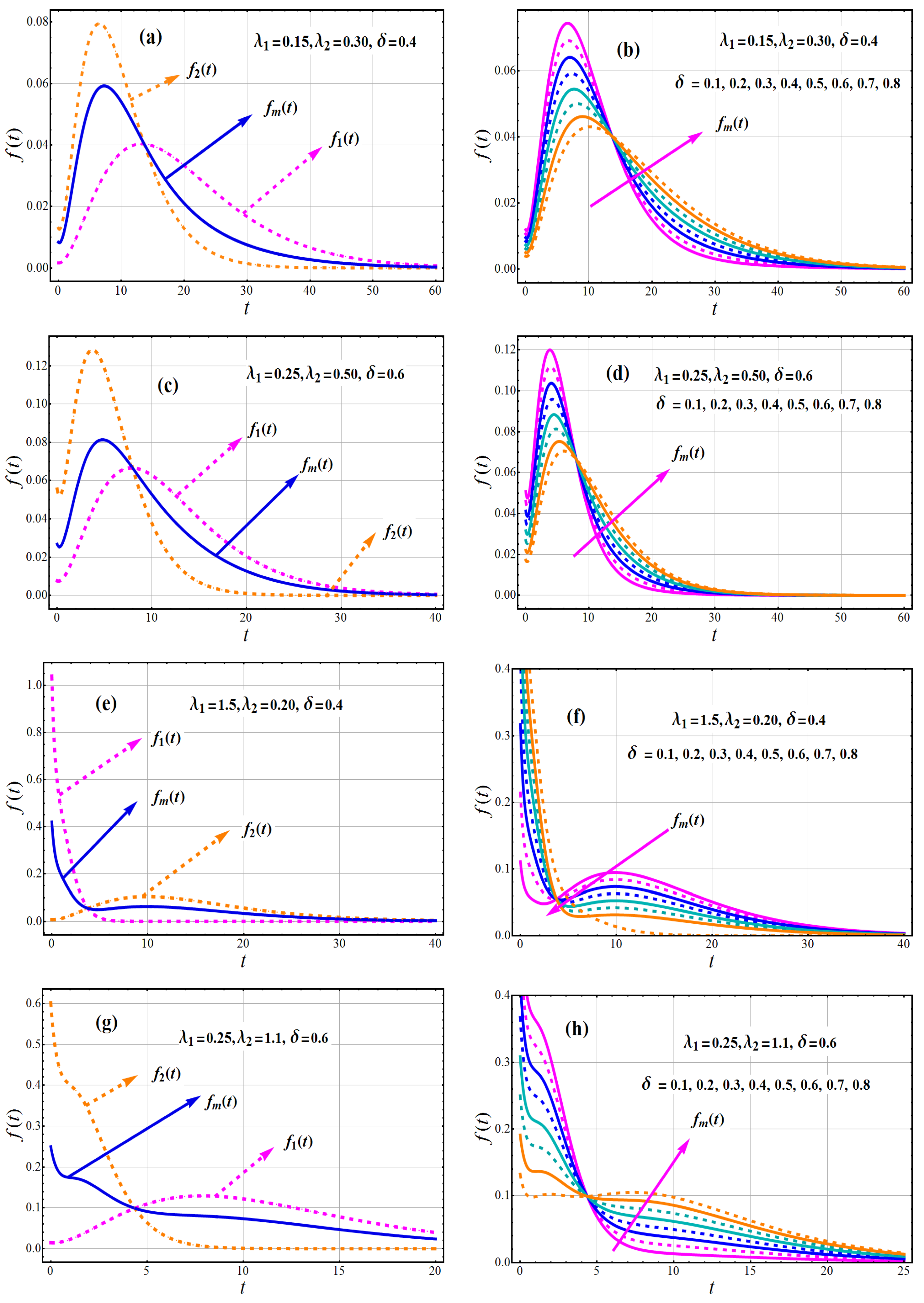
Figure 2.
Behavior of (first component CDF), (second component CDF) and CDF of TC-MAM ) with against t.
Figure 2.
Behavior of (first component CDF), (second component CDF) and CDF of TC-MAM ) with against t.
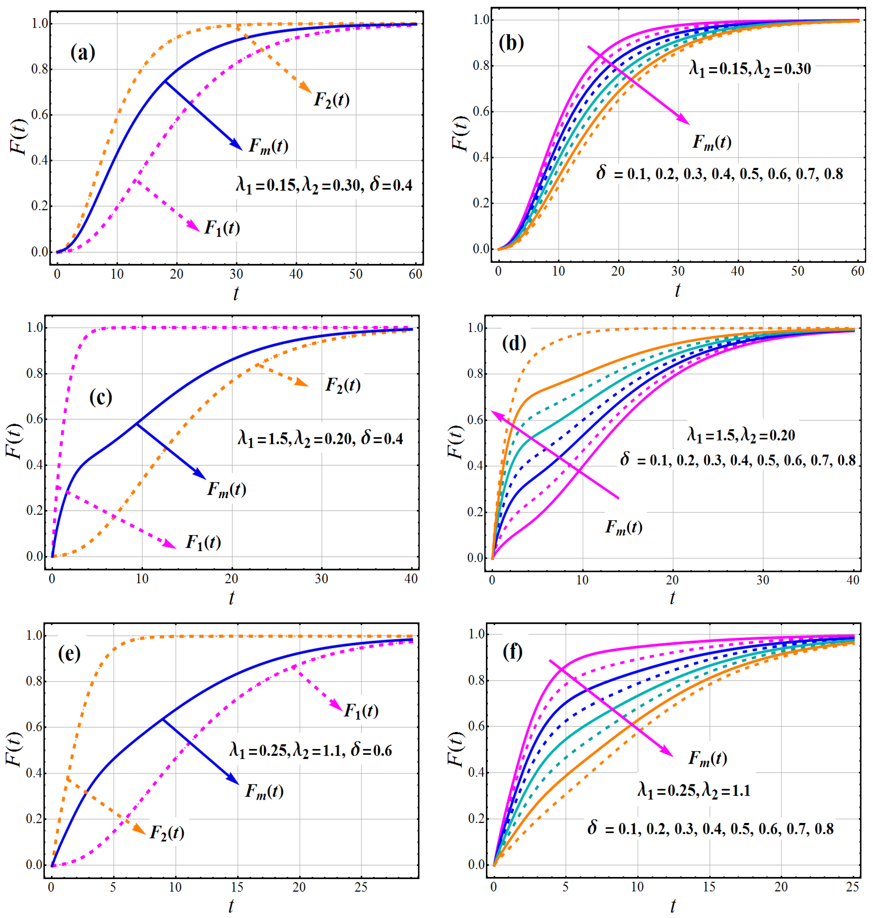
Figure 3.
Variations of Mean of TC-MAM.
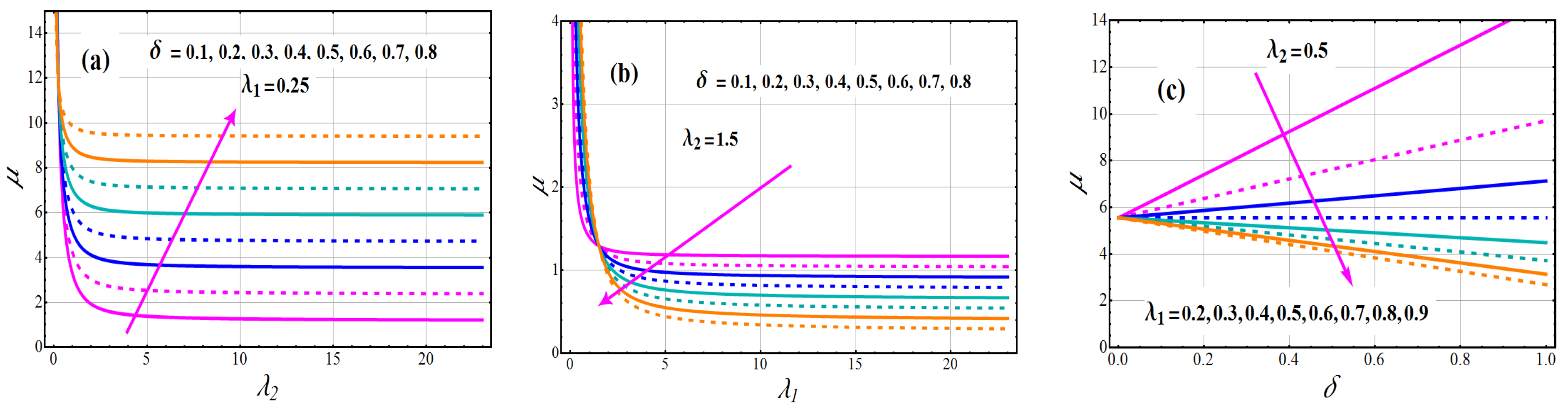
Figure 4.
Variations of Variance of TC-MAM.
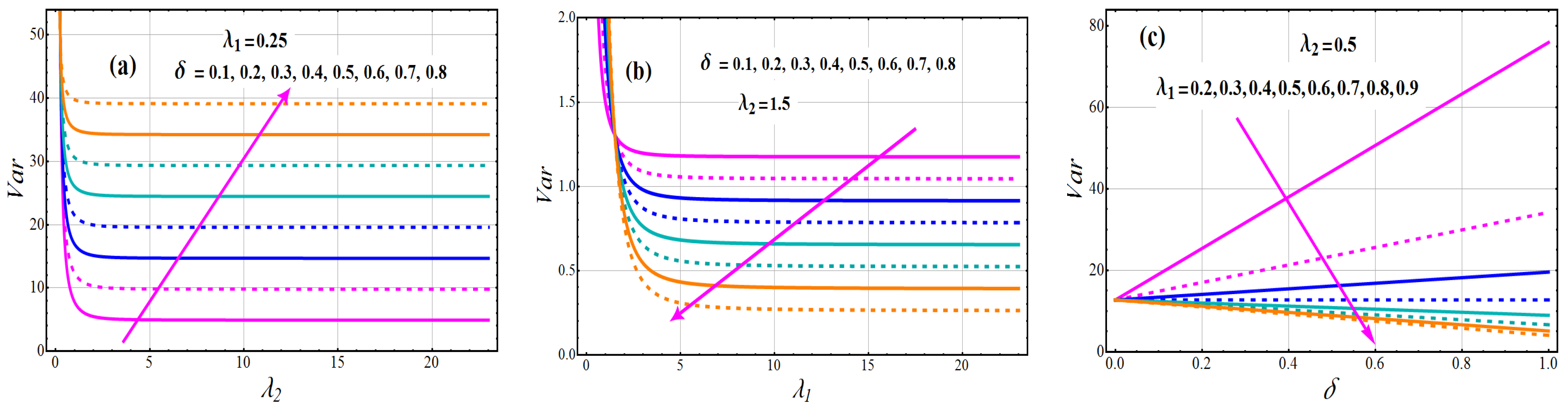
Figure 5.
Variations of index of dispersion of TC-MAM.
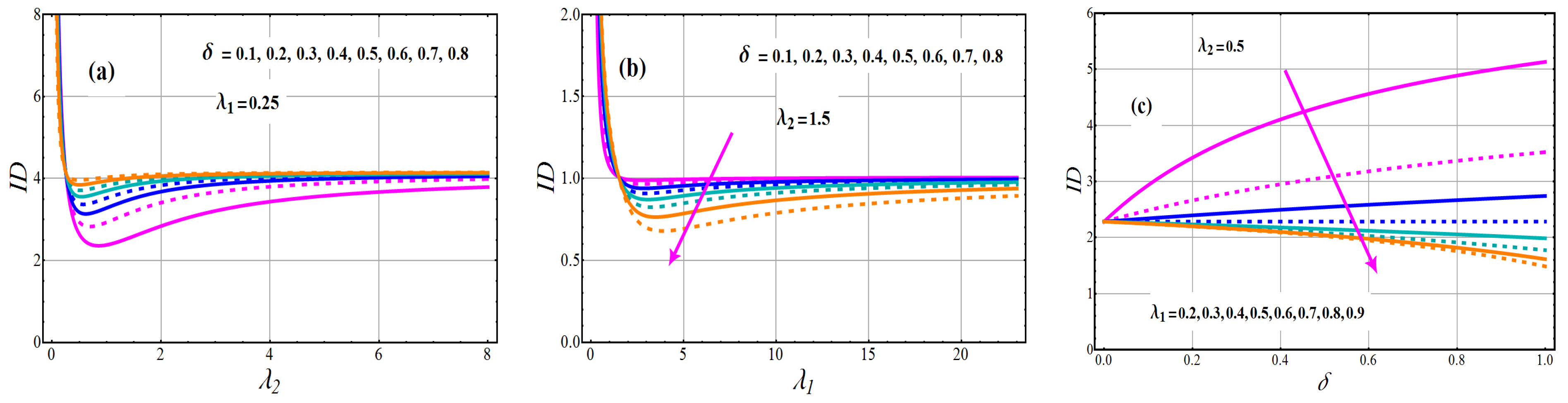
Figure 6.
Variations of coefficient of skewness , of TC-MAM.
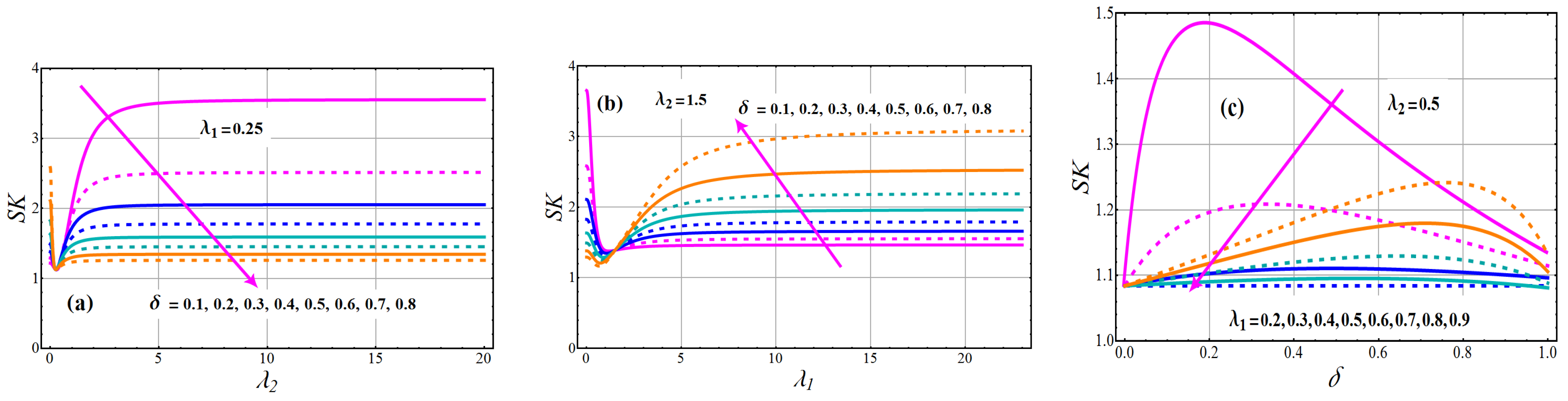
Figure 7.
Behavior of coefficient of kurtosis of TC-MAM.
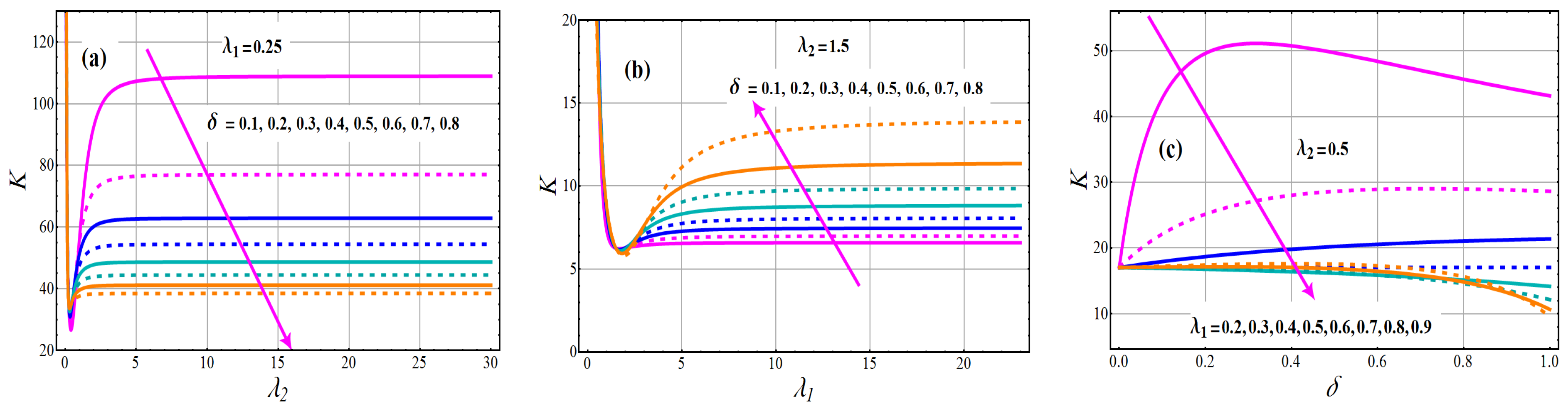
Figure 8.
Variations in for and .
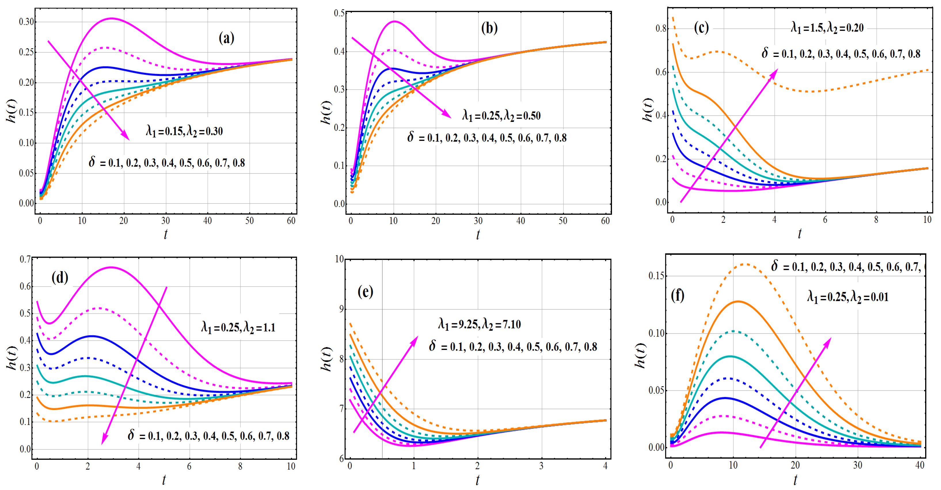
Figure 9.
Behavior of bias of estimators with different methods under parametric set I against n.
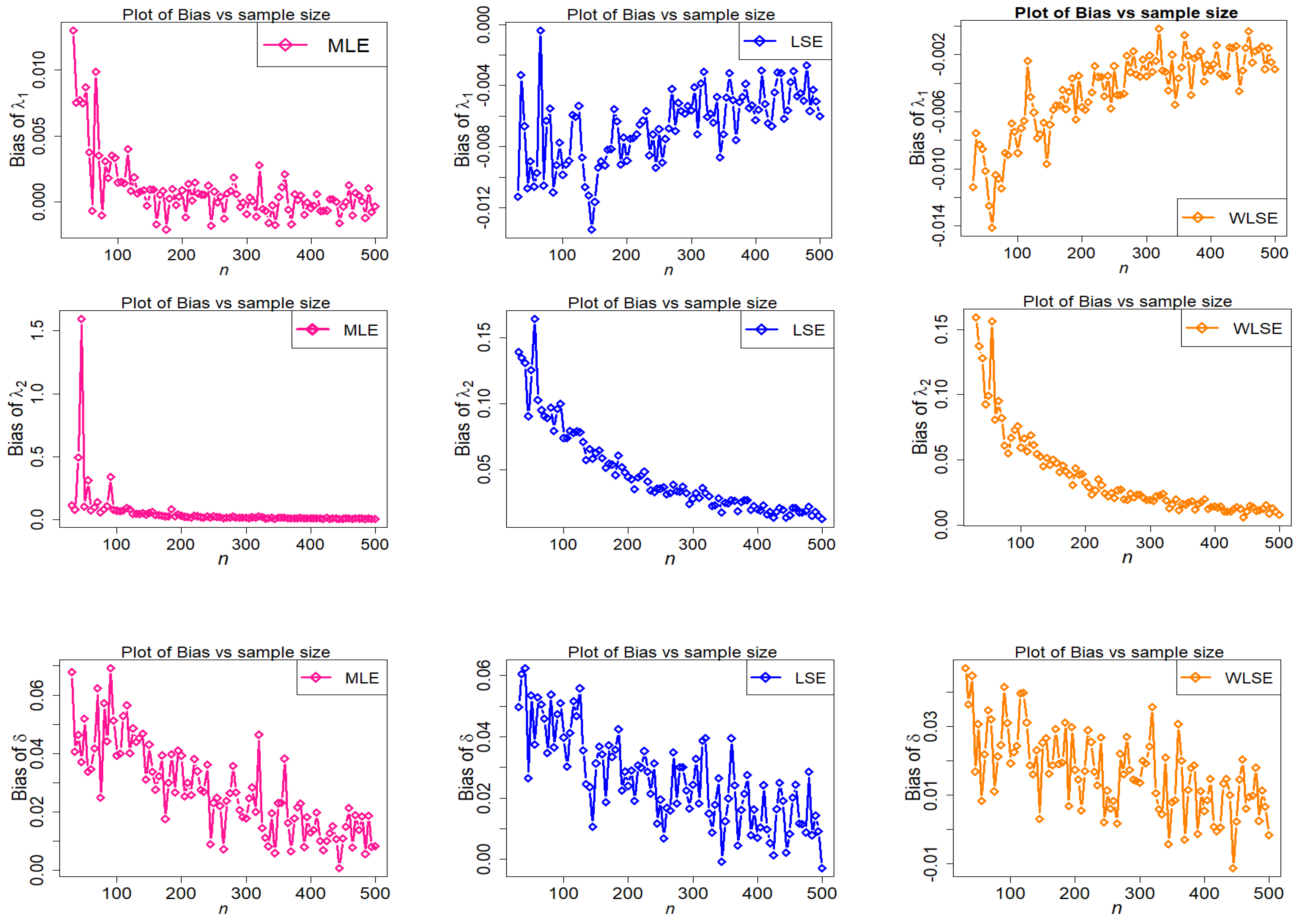
Figure 10.
Behavior of MSE of estimators with different methods under parametric set I against n.
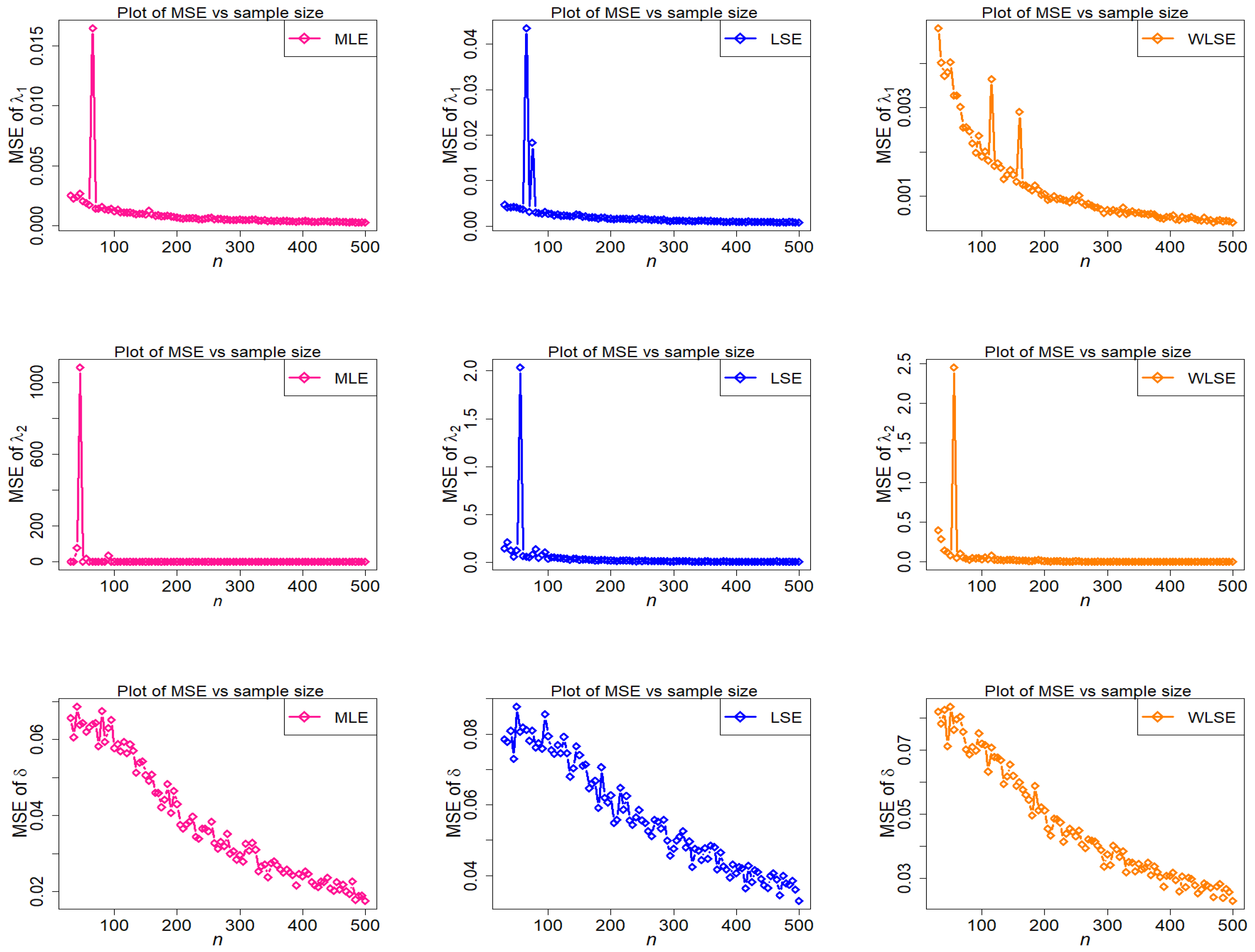
Figure 11.
Behavior of bias of estimators with different methods under parametric set II against n.
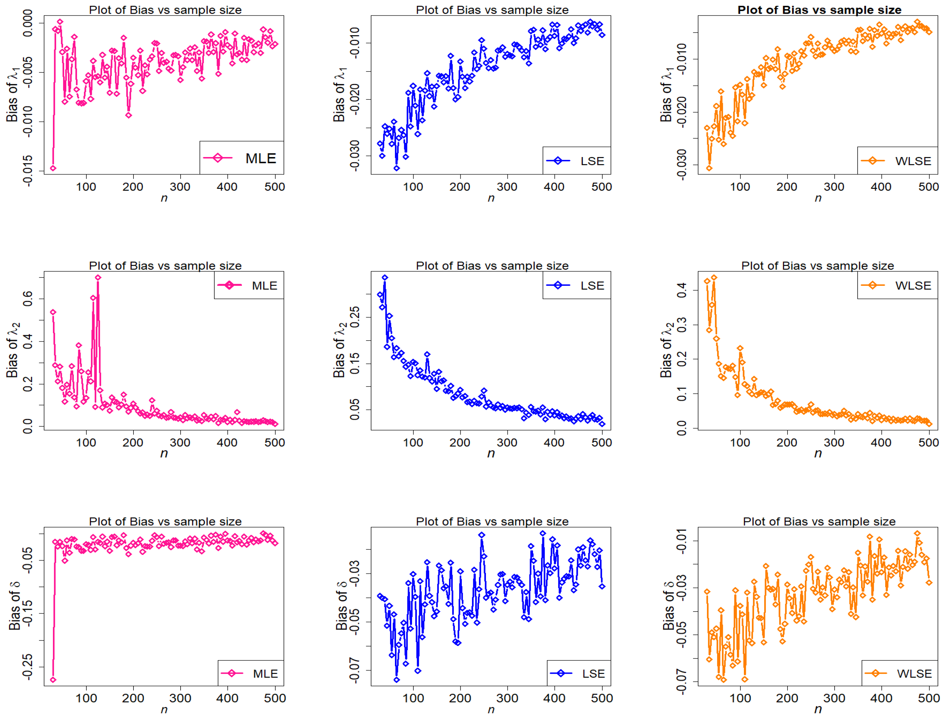
Figure 12.
Behavior of MSE of estimators with different methods under parametric set II against n.

Figure 13.
Behavior of bias of estimators with different methods under parametric set III against n.
Figure 13.
Behavior of bias of estimators with different methods under parametric set III against n.
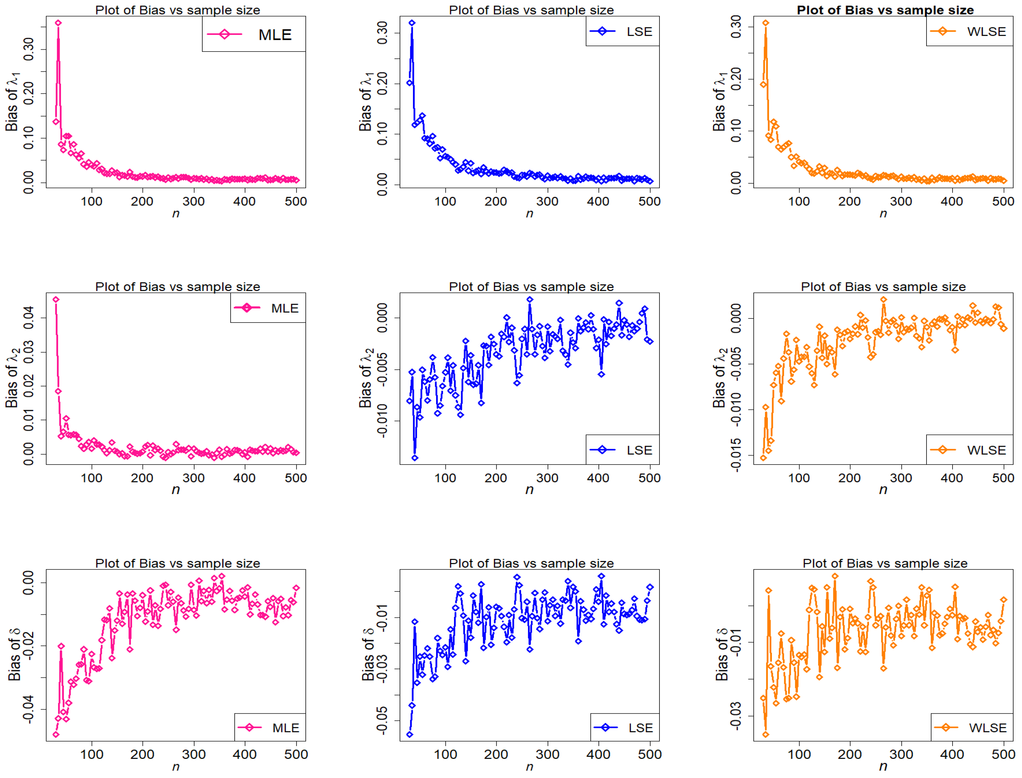
Figure 14.
Behavior of MSE of estimators with different methods under parametric set III against n.
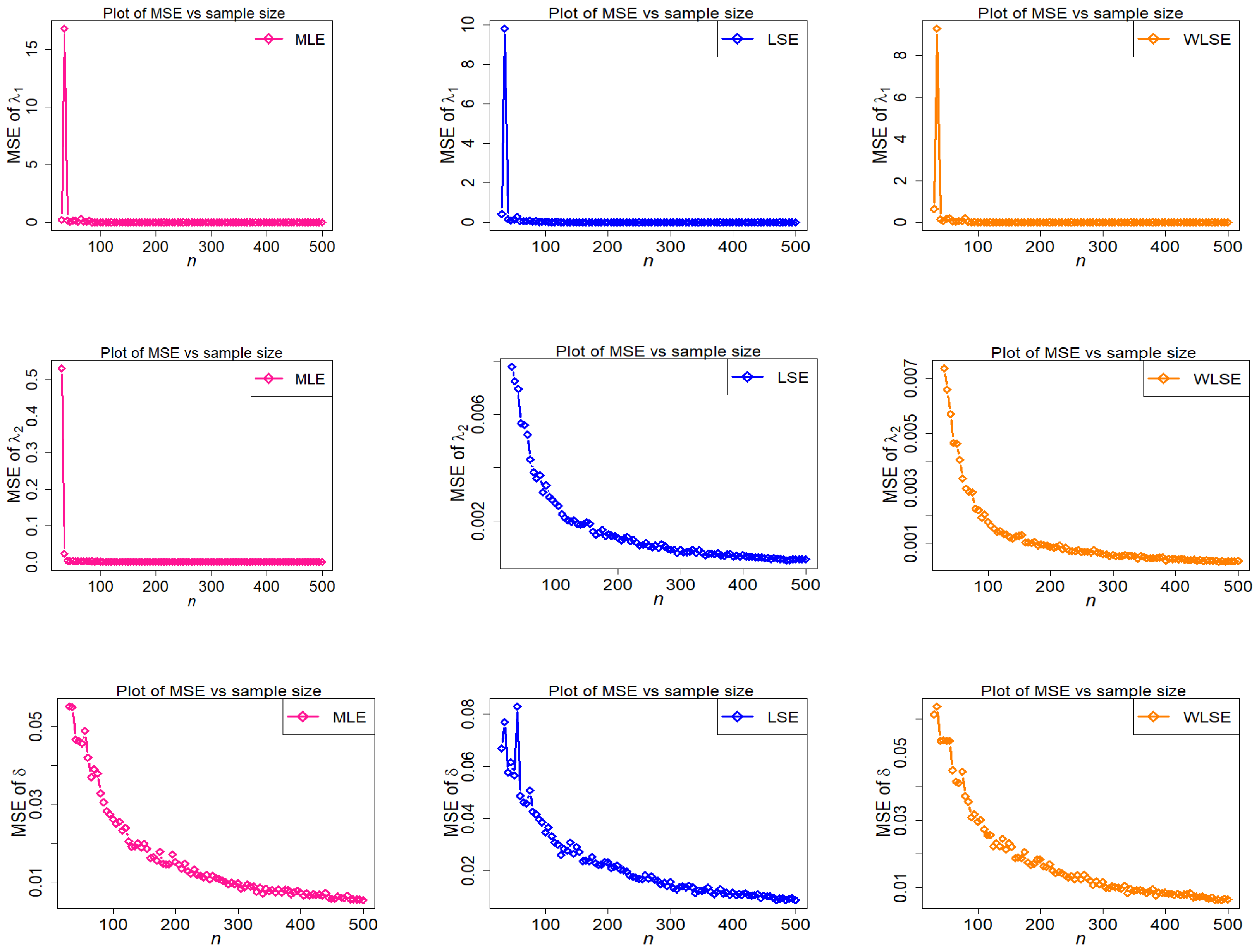
Figure 15.
The plots of PLLF for Dataset.
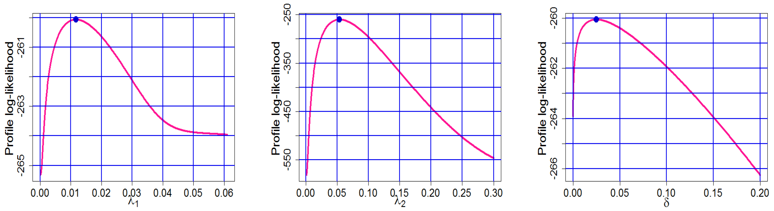
Figure 16.
The graphs of score functions cross the horizontal axis at and of Dataset.


Table 1.
MLEs, and GoF statistics for the Dataset I.
| Distributions | MLEs | AIC | BIC | AICC | ||
|---|---|---|---|---|---|---|
| TC-MAM | 0.011647 | 260.0557 | 526.1114 | 532.1875 | 526.5729 | |
| 0.053562 | ||||||
| 0.024836 | ||||||
| 2C-MSM | 0.008656 | 269.2051 | 544.4102 | 550.4863 | 544.8717 | |
| 0.035161 | ||||||
| 0.023762 | ||||||
| 2C-MLM | 0.008684 | 270.0022 | 546.0045 | 552.0805 | 546.4659 | |
| 0.034539 | ||||||
| 0.023282 | ||||||
| 2C-MEM | 0.016401 | 286.1761 | 578.3523 | 584.4283 | 578.8137 | |
| 0.016396 | ||||||
| 0.746712 | ||||||
Publisher’s Note: MDPI stays neutral with regard to jurisdictional claims in published maps and institutional affiliations. |
© 2022 by the authors. Licensee MDPI, Basel, Switzerland. This article is an open access article distributed under the terms and conditions of the Creative Commons Attribution (CC BY) license (https://creativecommons.org/licenses/by/4.0/).
Share and Cite
MDPI and ACS Style
Shafiq, A.; Sindhu, T.N.; Lone, S.A.; Hassan, M.K.H.; Nonlaopon, K. Mixture of Akash Distributions: Estimation, Simulation and Application. Axioms 2022, 11, 516. https://doi.org/10.3390/axioms11100516
AMA Style
Shafiq A, Sindhu TN, Lone SA, Hassan MKH, Nonlaopon K. Mixture of Akash Distributions: Estimation, Simulation and Application. Axioms. 2022; 11(10):516. https://doi.org/10.3390/axioms11100516
Chicago/Turabian StyleShafiq, Anum, Tabassum Naz Sindhu, Showkat Ahmad Lone, Marwa K. H. Hassan, and Kamsing Nonlaopon. 2022. "Mixture of Akash Distributions: Estimation, Simulation and Application" Axioms 11, no. 10: 516. https://doi.org/10.3390/axioms11100516
Note that from the first issue of 2016, this journal uses article numbers instead of page numbers. See further details here.