Digital h-Fibrations and Some New Results on Digital Fibrations

Abstract

In this work, the notion of digital fiber homotopy is defined and its properties are given. We present some new results on digital fibrations. Moreover, we introduce digital h-fibrations. We prove some of the properties of these digital h-fibrations. We show that a digital fibration and a digital map p are fiber homotopic equivalent if and only if p is a digital h-fibration. Finally, we explore a relation between digital fibrations and digital h-fibrations.

1. Introduction

Digital topology is interested in the relations among the subsets of ${\mathbb{Z}}^n$, where $\mathbb{Z}$ is the set of all integers. These sets are called digital images and they have some topological properties. Topological relations (such as digital homotopy, digital homology groups, etc.) between any two digital images allow us to deduce some information about one of the digital images by looking at the other one. Therefore, digital topology is used in the area of digital image processing.

At the beginning, Rosenfeld introduced digital topology [1,2]. In the following years, Boxer defined some algebraic topological methods on digital topology such as homotopy and fundamental groups [3,4,5,6,7].

The notion of homotopy theory in digital spaces has been continuously expanded upon into the current day [8,9,10]. Arslan et al. [11] defined digital homology groups. Karaca and Ege expanded on digital homology theory [12]. Karaca and Vergili [13] introduced the digital fiber bundle, which is another algebraic topological topic [14]. Homology groups in algebraic topology are used to classify topological spaces up to homeomorphism. Fiber bundles that are used to compute homology groups are significant tools in topology. Thus, Ege [15] introduced the concept of digital fibration, which is a generalization of the digital fiber bundle. This work deals with some of the properties that hold in algebraic topology but do not necessarily exist in digital topology. Some of the differences arose because only integers are used in digital topology. Therefore, it is necessary to understand digital topology in order to understand the relationships between digital images. (For recent studies on digital images, see [16,17,18,19].)

In algebraic topology, fiber homotopy is a homotopy that preserves fibers [20]. Since fibrations are not invariant under fiber homotopic equivalence, a map that is fiber homotopic to a fibration does not have to be a fibration. Thus, the homotopy lifting property (hlp) was changed and the weak homotopy lifting property was introduced by Dold [21]. By using the notion of the weak homotopy lifting property, Tajik et al. [22] introduced h-fibration and presented the relations between fibrations and h-fibrations.

These developments in algebraic topology have led us to investigate whether they are also valid in digital topology. In this work, we interpret fiber homotopy in terms of digital topology. This interpretation allows us to define digital h-fibrations. Moreover, some of the categorical properties of digital fibrations are presented.

The structure of this paper is organized as follows: In the next section, we provide the background information regarding digital topology such as adjacency relations, continuity, homotopy, fiber bundles, and fibrations. In the third section, we present the definitions and properties about digital fiber homotopy and give some new results on digital fibrations. In the final section, we introduce digital h-fibrations and prove its properties. We also provide a relation between digital h-fibrations and digital fibrations.

2. Preliminaries

Some basic definitions related to digital topology will be explained in this section.

Definition 1 

([3]). Let $n\in {\mathbb{Z}}^{+}$ and ${\mathbb{Z}}^n$ be a set that equals the n-times product of $\mathbb{Z}$. Supposing $a=(a_1,a_2,\dots ,a_n)$ and $b=(b_1,b_2,\dots ,b_n),then\in {\mathbb{Z}}^n$ and $u\in \mathbb{Z}$ with $1\le u\le n$. If there exist at most u indices i, such that $a_i$ and $b_i$ are consecutive integers and are otherwise equal, then we say a and b are $c_u$-adjacent.

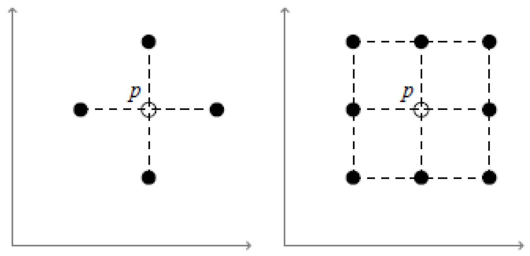
In general, adjacency $c_u$ is denoted by $q\in \mathbb{Z}$, where q is the number of points that are adjacent to a given point in ${\mathbb{Z}}^n$. As an example, $c_1=2$ in $\mathbb{Z}$. Moreover in ${\mathbb{Z}}^2$, $c_1$ and $c_2$ are 4 and 8, respectively (see Figure 1) [6].

Figure 1. In ${\mathbb{Z}}^2$, we have 4-adjacency and 8-adjacency, respectively.

Consider a set X in ${\mathbb{Z}}^n$ with an adjacency relation $\kappa$ on itself. Then, the pair $(X,\kappa )$ is called a digital image.

Definition 2 

([23]). Let $x_i,y_i\in (X_i,{\kappa }_i)$. In $X_0\times X_1$, given the two points $(x_0,x_1)$ and $(y_0,y_1)$ are adjacent if and only if any of the statements below holds:

(1) 

$x_0=y_0$, then $x_1$ and $y_1$ are ${\kappa }_1$-adjacent; or

(2) 

$x_1=y_1$, then $x_0$ and $y_0$ are ${\kappa }_0$-adjacent; or

(3) 

$x_0$ and $y_0$ are ${\kappa }_0$-adjacent, and $x_1$ and $y_1$ are ${\kappa }_1$-adjacent.

• Often, the adjacency of the Cartesian product of digital images is denoted by ${\kappa }_{\ast }$.

Definition 3 

([24]). Let $(A,{\lambda }_1)$, $(B,{\lambda }_2)$ be digital images and the $map(A,B)$ be a digital map space that includes digital maps from A to B. For $f,g\in map(A,B)$, we say that f and g are adjacent if $f\left(x_1\right)$ and $g\left(x_2\right)$ are ${\lambda }_2$-adjacent whenever $x_1$ and $x_2$ are ${\lambda }_1$-adjacent.

For $m,n\in \mathbb{Z}$, the set ${[m,n]}_{\mathbb{Z}}=\{z\in \mathbb{Z}|m\le z\le n\}$ is said to be a digital interval [3].

Consider an adjacency relation $\lambda$ on ${\mathbb{Z}}^n$. Then, we say a digital image X, which is a subset of ${\mathbb{Z}}^n$, is $\lambda$-connected if and only if for every distinct points $m,n\in X$, there exists a set $\{m_0,m_1,\dots ,m_r\}\subset X$ such that $m_0=m$, $m_r=n$ and $m_i$ and $m_{i+1}$ are $\lambda$-adjacent where $i\in {[0,r-1]}_{\mathbb{Z}}$ [4].

Definition 4 

([4]). Let $(A,{\lambda }_0)$ and $(B,{\lambda }_1)$ be digital images. For a map $p:A\to B$, if for all ${\lambda }_0$-connected $U\subset A$, $p\left(U\right)\subset B$ is a ${\lambda }_1$-connected, then p is called to be $({\lambda }_0,{\lambda }_1)$-continuous.

Definition 5 

([25]). Let $(A,\lambda )$ be a digital image. $\alpha :{[0,n]}_{\mathbb{Z}}\to A$ is called a digital $(2,\kappa )$-path if it is $(2,\lambda )$-continuous.

Consider that $(A,{\lambda }_0)$ and $(B,{\lambda }_2)$ are digital images. A function $p:A\to B$ is called $({\lambda }_0,{\lambda }_1)$-isomorphism—and is denoted by $A{\cong }_{({\lambda }_0,{\lambda }_1)}B$—if p is one to one and onto $({\lambda }_0,{\lambda }_1)$-continuous, and $p^{-1}$ is $({\lambda }_1,{\lambda }_0)$-continuous [7].

Definition 6 

([4]). Let $(A,{\lambda }_0)$, $(B,{\lambda }_1)$ be digital images. Two $({\lambda }_0,{\lambda }_1)$-continuous map $p,q:A\to B$ are called to be digitally $({\lambda }_0,{\lambda }_1)$-homotopic in B if there is $n\in {\mathbb{Z}}^{+}$ and there exists a map $K:A\times {[0,n]}_{\mathbb{Z}}\to B$ that satisfies each of the statements below:

(1) 

For all $a\in A$, $K(a,0)=p\left(a\right)$ and $K(a,n)=q\left(a\right)$;

(2) 

For all $a\in A$ and every $t\in {[0,n]}_{\mathbb{Z}}$, $K_a:{[0,n]}_{\mathbb{Z}}\to B$ is defined by $K_a\left(t\right)=K(a,t)$, which is $(2,{\lambda }_1)$-continuous;

(3) 

For all $a\in A$ and every $t\in {[0,n]}_{\mathbb{Z}}$, $K_t:A\to B$ is defined by $K_t\left(a\right)=K(a,t)$, which is $({\lambda }_0,{\lambda }_1)$-continuous.

• Also, K is called a digital $({\lambda }_0,{\lambda }_1)$-homotopy between p and q.

Definition 7 

([13]). Let $(E,{\lambda }_1)$ and $(B,{\lambda }_2)$ be digital images where B is a ${\lambda }_2$-connected space. Then, we say $(E,p,B)$ is a digital bundle if the map $p:E\to B$ is a $({\lambda }_1,{\lambda }_2)$-continuous surjection. B, E and p are called the base set, total set and the digital projection of the bundle, respectively. In addition, the digital fiber bundle of the bundle over t is defined by $p^{-1}\left(t\right)$ for every $t\in B$.

Definition 8 

([13]). Let $(E,{\lambda }_1)$, $(B,{\lambda }_2)$ and $(F,{\lambda }_3)$ be digital images, where B is a connected space with ${\lambda }_2$-adjacency. Consider a surjection and a $({\lambda }_1,{\lambda }_2)$-continuous map $p:E\to B$. For a digital fiber set F, if there is a set $U\subset B$ that is ${\lambda }_2$-connected and p satisfies the statements below, then $\xi =(E,p,B,F)$ is a digital fiber bundle.

(1) 

For each $t\in B$, $p^{-1}\left(t\right)\to F$ is a $({\lambda }_1,{\lambda }_3)$-isomorphism

(2) 

For all $t\in B$, there is a $({\lambda }_1,{\lambda }^{\ast })$-isomorphism $\varphi :p^{-1}\left(U\right)\to U\times F$ that makes triangles below commutes:

In the following definition, the digital homotopy lifting property is given to define the digital fibration.

Definition 9 

([15]). Let i be an inclusion map and $n\in {\mathbb{Z}}^{+}$ for any digital homotopy $T:X\times {[0,n]}_{\mathbb{Z}}\to B$ and any digital map $\tilde{g}:X\to E$ with $p\circ \tilde{g}=T\circ i$, where $(E,{\lambda }_1)$, $(B,{\lambda }_2)$ and $(X,{\lambda }_3)$ are digital images. Then, we say $p:E\to B$ has the digital hlp with respect to $(X,{\lambda }_3)$ if there is a digital $({\lambda }^{\ast },{\lambda }_1)$-continuous map $\tilde{T}$ making the following triangles below commute:

Definition 10 

([15]). For a digital map $p:(E,{\lambda }_1)\to (B,{\lambda }_2)$, p is called a digital fibration if it has the digital hlp with respect to each space $(X,{\lambda }_3)$. For $t\in B$, $p^{-1}\left(t\right)$, it is called digital fiber.

3. Digital Fiber Homotopy

Fiber homotopy is an important topic in algebraic topology. In this section, we define digital fiber homotopy and its properties are proven. In addition, some new results about digital fibrations are given.

Definition 11. 

For a digital map $q:(A,\kappa )\to (B,\lambda )$, if ${\alpha }_1$ and ${\alpha }_2$ are two digital paths in A such that $q\circ {\alpha }_1=q\circ {\alpha }_2$ and ${\alpha }_1\left(0\right)={\alpha }_2\left(0\right)$ implies that ${\alpha }_1={\alpha }_2$, then q has a digital unique path lifting property (upl).

Definition 12. 

Let $f,g:(A,{\lambda }_3)\to (E,{\lambda }_1)$ and $q:(E,{\lambda }_1)\to (B,{\lambda }_2)$ be three digital maps. Then, we say that f and g are digital fiber homotopic with respect to q, which is represented by $f{\simeq }_{q}g$, if there exists a digital homotopy $K:f\simeq g$ such that

$$q\circ K(a,t)=q\circ f\left(a\right)=q\circ g\left(a\right)$$

for every $a\in A$ and every $t\in {[0,n]}_{\mathbb{Z}}$. Here, K is called digital fiber homotopic between f and g.

Example 1. 

Let $q:E\to B$ be a digital map, and let $f,g:(X,{\kappa }_3)\to (E,{\kappa }_1)$ be two digital maps that are digital homotopic to each other. If B is a singleton, then $f{\simeq }_{q}g$.

Example 2. 

Consider $X=\{1,2,3\}\subset \mathbb{Z}$, $E=\{(0,0),(0,1),(1,0)\}\subset {\mathbb{Z}}^2$ and

$B=\{0,1\}\subset \mathbb{Z}$. Let $f,g:(X,{\kappa }_3)\to (E,{\kappa }_1)$ be defined by

$$f\left(1\right)=(0,0),f\left(2\right)=(1,0),f\left(3\right)=(0,1),$$

$$g\left(1\right)=(0,0),g\left(2\right)=(0,1),g\left(3\right)=(1,0).$$

Suppose that $T:X\times {[0,2]}_{\mathbb{Z}}\to E$ satisfies the conditions below. Clearly, T is a digital homotopy.

$$T(m,0)=f\left(m\right),T(m,2)=g\left(m\right),$$

$$T(1,1)=(0,0),T(2,1)=(1,0),T(3,1)=(0,1).$$

Let $q:(E,{\kappa }_1)\to (B,{\kappa }_2)$ be defined by $q(e_1,e_2)=e_1+e_2$. Therefore, we obtain

$$q\circ T(m,t)=q\circ f\left(m\right)=q\circ g\left(m\right)$$

for every $m\in X$ and $t\in {[0,2]}_{\mathbb{Z}}$. As a result, we obtain f and g, which are fiber homotopic with respect to q.

Definition 13. 

Let $q_1:(A_1,{\kappa }_1)\to (B,\kappa )$ and $q_2:(A_2,{\kappa }_2)\to (B,\kappa )$ be digital maps. If $q_1=q_2\circ p$, then $p:(A_1,{\kappa }_1)\to (A_2,{\kappa }_2)$ is called the digital fiber preserving map.

Definition 14. 

Let $q_1:(A_1,{\kappa }_1)\to (B,\kappa )$ and $q_2:(A_2,{\kappa }_2)\to (B,\kappa )$ be digital maps. If there are two digital maps $p:(A_1,{\kappa }_1)\to (A_2,{\kappa }_2)$ and $p^{\prime }:(A_2,{\kappa }_2)\to (A_1,{\kappa }_1)$ that are fiber preserving such that $p^{\prime }\circ p{\simeq }_{q_1}i{d}_{A_1}$ and $p\circ p^{\prime }{\simeq }_{q_2}i{d}_{A_2}$, then we say $q_1$ and $q_2$ are digital fiber homotopic equivalent to each other. In addition, p and $p^{\prime }$ are said to be digital fiber homotopic equivalent.

Proposition 1. 

Let $p_1:(A,{\kappa }_1)\to (B,{\kappa }_2)$ be a digital map. If $p_2:(A^{\prime },{\kappa }_1^{\prime })\to (A,{\kappa }_1)$ and $s,s^{\prime }:(Y,\kappa )\to (A^{\prime },{\kappa }_1)$ are two digital maps such that $s{\simeq }_{p_2}{s}^{\prime }$, then $s{\simeq }_{p_1\circ p_2}{s}^{\prime }$.

Proof. 

Let $s{\simeq }_{p_2}{s}^{\prime }$. By assumption, for every $y\in Y$ and every $t\in {[0,m]}_{\mathbb{Z}}$, there exists a homotopy $G:s{\simeq }_{p_2}{s}^{\prime }$ such that $p_2\circ G(y,t)=p_2\circ s\left(y\right)=p_2\circ s^{\prime }\left(y\right)$. Therefore,

$$(p_1\circ p_2)\circ G(y,t)=p_1\circ (p_2\circ G(y,t))=p_1\circ (p_2\circ s\left(y\right))=(p_1\circ p_2)\circ s\left(y\right)$$

(1)

$$(p_1\circ p_2)\circ G(y,t)=p_1\circ (p_2\circ G(y,t))=p_1\circ (p_2\circ s^{\prime }\left(y\right))=(p_1\circ p_2)\circ s^{\prime }\left(y\right).$$

(2)

As a result, $G:s{\simeq }_{p_1\circ p_2}{s}^{\prime }$. □

Proposition 2. 

Digital fiber homotopy is an equivalence relation.

Proof. 

Consider the class $K=\left\{f\right|f:(Y,{\kappa }_1)\to (E,{\kappa }_2)\}$.

• If we choose $G:Y\times {[0,m]}_{\mathbb{Z}}\to E$ such that $G(a,t)=f\left(a\right)$, we have $f{\simeq }_{q}f$.
• Thus, the symmetry property is clear.
• Let $f{\simeq }_{q}g$ and $g{\simeq }_{q}h$. From the hypothesis, for all $t\in {[0,m]}_{\mathbb{Z}}$, there are two digital homotopies G and H satisfying the following:

  $$q\circ G(a,t)=q\circ f\left(a\right)=q\circ g\left(a\right),$$

  $$q\circ H(a,t)=q\circ g\left(a\right)=q\circ h\left(a\right).$$

By taking one of G and H as a homotopy, we have $f{\simeq }_{q}h$. □

Proposition 3. 

Let $s:(A,{\kappa }_1)\to (B,{\kappa }_2)$ be a digital map. If $f_1,f_2:(Z,\lambda )\to (A,{\kappa }_1)$ and $h:(X,\gamma )\to (Z,\lambda )$ are digital maps such that $f_1{\simeq }_s{f}_2$, then $f_1\circ h{\simeq }_s{f}_2\circ h$.

Proof. 

As an assumption, there is a digital fiber homotopy $K:f_1{\simeq }_s{f}_2$. Hence, we obtained

$$s\circ K(z,t)=s\circ f_1\left(z\right)=s\circ f_2\left(z\right).$$

Let $K^{\prime }:X\times {[0,m]}_{\mathbb{Z}}\to E$ be defined by $K^{\prime }(a,t)=K(h\left(a\right),t)$. Via the following equations,

$$K^{\prime }(a,0)=K(h\left(a\right),0)=f_1\circ h\left(a\right)$$

$$K^{\prime }(a,m)=K(h\left(a\right),m)=f_2\circ h\left(a\right),$$

we have $K^{\prime }:f_1\circ h\simeq f_2\circ h$. Thus, we obtain

$$s\circ K^{\prime }(a,t)=s\circ K(h\left(a\right),t)=s\circ f_1\left(h\left(a\right)\right)=s\circ (f_1\circ h)\left(a\right)$$

$$s\circ K^{\prime }(a,t)=s\circ K(h\left(a\right),t)=s\circ f_2\left(h\left(a\right)\right)=s\circ (f_2\circ h)\left(a\right).$$

As a result, $f_1\circ h{\simeq }_s{f}_2\circ h$. □

Proposition 4. 

Let $q_1:(E,{\kappa }_1)\to (B,{\kappa }_2)$ be a digital map. The existing digital maps $p_1,p_2:(A,\lambda )\to (E^{\prime },{\kappa }_1^{\prime })$ and $q_2:(E^{\prime },{\kappa }_1^{\prime })\to (E,{\kappa }_1)$ are such that $p_1{\simeq }_{q_1\circ q_2}{p}_2$ implies that $q_2\circ p_1{\simeq }_{q_1}{q}_2\circ p_2$.

Proof. 

Let $T:p_1{\simeq }_{q_1\circ q_2}{p}_2$. Hence,

$$q_1\circ q_2\circ T(a,t)=q_1\circ q_2\left(p_1\left(a\right)\right)=q_1\circ q_2\left(p_2\left(a\right)\right).$$

Let $T^{\prime }:A\times {[0,m]}_{\mathbb{Z}}\to E$ be defined by $T^{\prime }(a,t)=q_2\circ T(a,t)$. As such, we have

$$q_1\circ T^{\prime }(a,t)=q_1\circ q_2\circ T(a,t)=q_1\circ q_2\left(p_1\left(a\right)\right)=q_1\circ (q_2\circ p_1)\left(a\right)$$

$$q_1\circ T^{\prime }(a,t)=q_1\circ q_2\circ T(a,t)=q_1\circ q_2\left(p_2\left(a\right)\right)=q_1\circ (q_2\circ p_2)\left(a\right).$$

This shows that $T^{\prime }$ is digital fiber homotopic with respect to $q_1$. □

Proposition 5. 

Let $s_1:(E,{\kappa }_1)\to (B,{\kappa }_2)$ and $s_2:(E^{\prime },{\kappa }_1^{\prime })\to (B^{\prime },{\kappa }_2^{\prime })$ be digital maps. If $f_1,g_1:(X,\lambda )\to (E,{\kappa }_1)$ and $f_2,g_2:(X,\lambda )\to (E^{\prime },{\kappa }_1^{\prime })$ are digital maps such that $f_1{\simeq }_{s_1}{g}_1$ and $f_2{\simeq }_{s_2}{g}_2$, then $(f_1,f_2){\simeq }_{s_1\times s_2}(g_1,g_2)$.

Proof. 

Let $H:f_1{\simeq }_{s_1}{g}_1$ and $K:f_2{\simeq }_{s_2}{g}_2$. Then, we have the following:

$$s_1\circ H(x,t)=s_1\circ f_1\left(x\right)=s_1\circ g_1\left(x\right)$$

$$s_2\circ K(x,t)=s_2\circ f_2\left(x\right)=s_2\circ g_2\left(x\right).$$

We define $T:X\times {[0,m_2]}_{\mathbb{Z}}\to E\times E^{\prime }$ as

$$T(x,t)=\left\{\begin{array}{cc}\left(H\right(x,t),K(x,t\left)\right),\hfill & t\in {[0,m_1]}_{\mathbb{Z}}\hfill \\ (H(x,m_1),K(x,t)),\hfill & t\in {[m_1,m_2]}_{\mathbb{Z}}.\hfill \end{array}\right.$$

It is evident that T is a digital homotopy from $(f_1,f_2)$ to $(g_1,g_2)$. Using the digital fiber homotopy for H and K, we have the following equations. For $t\in {[0,m_1]}_{\mathbb{Z}}$,

$$\begin{array}{cc}\hfill (s_1\times s_2)\circ T(x,t)& =(s_1\circ H(x,t),s_2\circ K(x,t))\hfill \\ \hfill & =(s_1\circ f_1\left(x\right),s_2\circ f_2\left(x\right))\hfill \\ \hfill & =(s_1\times s_2)\circ (f_1,f_2)\left(x\right)\hfill \end{array}$$

(3)

$$\begin{array}{cc}\hfill (s_1\times s_2)\circ T(x,t)& =(s_1\circ H(x,t),s_2\circ K(x,t))\hfill \\ \hfill & =(s_1\circ g_1\left(x\right),s_2\circ g_2\left(x\right))\hfill \\ \hfill & =(s_1\times s_2)\circ (g_1,g_2)\left(x\right).\hfill \end{array}$$

(4)

For $t\in {[m_1,m_2]}_{\mathbb{Z}}$,

$$\begin{array}{cc}\hfill (s_1\times s_2)\circ T(x,t)& =(s_1\circ H(x,m_1),s_2\circ K(x,t))\hfill \\ \hfill & =(s_1\circ f_1\left(x\right),s_2\circ f_2\left(x\right))\hfill \\ \hfill & =(s_1\times s_2)\circ (f_1,f_2)\left(x\right)\hfill \end{array}$$

(5)

$$\begin{array}{cc}\hfill (s_1\times s_2)\circ T(x,t)& =(s_1\circ H(x,m_1),s_2\circ K(x,t))\hfill \\ \hfill & =(s_1\circ g_1\left(x\right),s_2\circ g_2\left(x\right))\hfill \\ \hfill & =(s_1\times s_2)\circ (g_1,g_2)\left(x\right).\hfill \end{array}$$

(6)

As a result, we have $(f_1,f_2){\simeq }_{s_1\times s_2}(g_1,g_2)$. □

Definition 15. 

Let $m\in \mathbb{Z}$ and $(Y,\lambda )$ be a digital image. A digital path space is defined as a set of digital paths that are from ${[0,m]}_{\mathbb{Z}}$ to Y and are denoted by $Y^{{[0,m]}_{\mathbb{Z}}}$. In addition, for a given digital map $f:(X,\kappa )\to (Y,\lambda )$, $P_f=\left\{(x,\alpha )\right|f\left(x\right)=\alpha \left(0\right)\}\subset X\times Y^{{[0,m]}_{\mathbb{Z}}}$ is said to be a digital mapping path space.

Let $p_0:(Y^{{[0,m]}_{\mathbb{Z}}},{\lambda }^{\ast })\to (Y,{\lambda }^{\prime })$ be a digital fibration defined by $p_0\left(\alpha \right)=\alpha \left(0\right)$, and let $f:(X,\lambda )\to (Y,{\lambda }^{\prime })$ be a digital map. Suppose that $p:P_f\to X$ is a digital fibration. Then, p is called a digital mapping path fibration of f, if it is induced from $p_0$ by f. There exists a section map from X to $P_f$ that is defined by $s\left(x\right)=(x,{\alpha }_{f\left(x\right)})$. Here, ${\alpha }_{f\left(x\right)}$ is a constant path in Y at $f\left(x\right)$. Consider a digital map $p_1:P_f\to Y$ that is defined by $p_1(x,\alpha )=\alpha \left(m\right)$.

Proposition 6. 

Let $f:(X,\kappa )\to (Y,{\kappa }^{\prime })$ be a digital map. Let $p_1$ and s be defined as before. Then, there exists a commutative diagram satisfying the following:

i.$1_{P_f}{\simeq }_{p}s\circ p$,

ii.$p_1$ is a digital fibration.

Proof. i. 

Consider $T:P_f\times {[0,m]}_{\mathbb{Z}}\to P_f$ to be defined by $T((x,\alpha ),t)=(x,{\alpha }_t)$, where

$${\alpha }_t\left(s\right)=\left\{\begin{array}{cc}\alpha \left(o\right),\hfill & s=0\hfill \\ \alpha \left(s\right),\hfill & s\ne 0.\hfill \end{array}\right.$$

Since $(x,\alpha )\in P_f$, $f\left(x\right)=\alpha \left(0\right)$, then—via the definition of ${\alpha }_t$, $\alpha \left(0\right)={\alpha }_t\left(0\right)$—we have $(x,{\alpha }_t)\in P_f$. Moreover, we also have

• $p\circ T((x,\alpha ),t)=p(x,{\alpha }_t)=x$,
• $p\circ 1_{P_f}(x,\alpha )=p(x,\alpha )=x$,
• $p\circ s\circ p(x,\alpha )=p\circ s\left(x\right)=p(x,{\alpha }_{f\left(x\right)})=x$.

• As a result, $1_{p_f}{\simeq }_{p}s\circ p$.

ii. Let $g:A\to P_f$ and $G:A\times {[0,m]}_{\mathbb{Z}}\to Y$ be maps such that $G(\alpha ,t)=p_1\circ g\left(\alpha \right)$ for $\alpha \in A$. That is to say that the diagram below is commutative.

There are two digital maps $g^{\prime }:A\to X$ and $g^{″}:A\to Y^{{[0,m]}_{\mathbb{Z}}}$ such that

$$g^{″}\left(\alpha \right)\left(0\right)=f\circ g^{\prime }\left(\alpha \right)\mathrm{and}g\left(\alpha \right)=(g^{\prime }\left(\alpha \right),g^{″}\left(\alpha \right)).$$

Now, we define a lifting function $\tilde{G}:A\times {[0,n]}_{\mathbb{Z}}\to P_f$ by $\tilde{G}(\alpha ,t)=(g^{\prime }\left(\alpha \right),\overline{g}(\alpha ,t))$, where $\overline{g}(\alpha ,t)\in Y^{{[0,n]}_{\mathbb{Z}}}$ is defined by

$$\overline{g}(\alpha ,t)\left(t^{\prime }\right)=\left\{\begin{array}{cc}{g}^{″}\left(\alpha \right)\left(t\right),\hfill & t^{\prime }\in {[0,m]}_{\mathbb{Z}}\hfill \\ G(\alpha ,t),\hfill & t^{\prime }\in {[m,n]}_{\mathbb{Z}}.\hfill \end{array}\right.$$

For $t^{\prime }\in {[0,m]}_{\mathbb{Z}}$,

$$p_1\circ \tilde{G}(\alpha ,t)=p_1(g^{\prime }\left(\alpha \right),\overline{g}(\alpha ,t))=\overline{g}(\alpha ,t)\left(m\right)=g^{″}\left(\alpha \right)\left(m\right)=p_1\circ g\left(\alpha \right)=G(\alpha ,t).$$

For $t^{\prime }\in {[m,n]}_{\mathbb{Z}}$,

$$p_1\circ \tilde{G}(\alpha ,t)=G(\alpha ,t).$$

Thus, we have $p_1\circ \tilde{G}=G$.

For fiber homotopy, if $t^{\prime }\in {[0,m]}_{\mathbb{Z}}$, then

$$\begin{array}{cc}\hfill \tilde{G}\circ i\left(\alpha \right)& =\tilde{G}(\alpha ,t)\hfill \\ \hfill & =(g^{\prime }\left(\alpha \right),\overline{g}(\alpha ,t))\hfill \\ \hfill & =g\left(\alpha \right).\hfill \end{array}$$

(7)

If $t^{\prime }\in {[m,n]}_{\mathbb{Z}}$, then

$$\begin{array}{cc}\hfill \tilde{G}\circ i\left(\alpha \right)& =\tilde{G}(\alpha ,t)\hfill \\ \hfill & =(g^{\prime }\left(\alpha \right),\overline{g}(\alpha ,t))\hfill \\ \hfill & =(g^{\prime }\left(\alpha \right),G(\alpha ,t))\hfill \\ \hfill & =(g^{\prime }\left(\alpha \right),p_1\circ g\left(\alpha \right))\hfill \\ \hfill & =(g^{\prime }\left(\alpha \right),g^{″}\left(\alpha \right)\left(m\right))\hfill \\ \hfill & =g\left(\alpha \right).\hfill \end{array}$$

(8)

Hence, $\tilde{G}\circ i=g$, and we thus conclude that $p_1$ is a digital fibration. □

Definition 16. 

Let $f:(B^{\prime },{\lambda }^{\prime })\to (B,\lambda )$ and $p:(E,\kappa )\to (B,\lambda )$ be digital maps. The digital fiber product of $B^{\prime }$ and E is known as $E^{\prime }$, and it is defined by

$$E^{\prime }=\left\{(b^{\prime },e)\right|f\left(b^{\prime }\right)=p\left(e\right)\}\subset B^{\prime }\times E.$$

It should be noted there exist two digital maps $f^{\prime }:(E^{\prime },{\kappa }^{\ast })\to (E,\kappa )$ and $p^{\prime }:(E^{\prime },{\kappa }^{\ast })\to (B^{\prime },{\lambda }^{\prime })$ that are defined by $f^{\prime }(b^{\prime },e)=e$ and $p^{\prime }(b^{\prime },e)=b^{\prime }$, respectively.

In category theory, $E^{\prime }$, $f^{\prime }$ and $p^{\prime }$ are characterized as the digital product of f and p. Here, continuous maps with a range B are objects of category, and they are also morphisms of the below category commute triangle:

As such, we have the following properties.

Proposition 7. 

Consider the above definition.

i. 

If p is injective (or surjective), then $p^{\prime }$ is injective (or surjective).

ii. 

Then, a digital trivial fibration from $B^{\prime }\times F$ to $B^{\prime }$ and $p^{\prime }:E^{\prime }\to B$ are digital fiber homotopic equivalent to each other, if $p:B\times F\to B$ is a digital trivial fibration.

iii. 

If p is a digital fibration (wupl), then so is $p^{\prime }$.

iv. 

Suppose p is a digital fibration, then $p^{\prime }$ has a section if and only if f can be lifted to E.

Proof. i. 

Let $X_1=E$ and $X_2=B^{\prime }$. Suppose that p is injective. Let $(b_1^{\prime },e_1),(b_2^{\prime },e_2)\in E^{\prime }$. By the definition of $E^{\prime }$, $f\left(b_1^{\prime }\right)=p\left(e_1\right)$, $f\left(b_2^{\prime }\right)=p\left(e_2\right)$. If $p^{\prime }(b_1^{\prime },e_1)=p^{\prime }(b_2^{\prime },e_2)$, then $b_1^{\prime }=b_2^{\prime }$.

Therefore, we have $p\left(e_1\right)=f\left(b_1^{\prime }\right)=f\left(b_2^{\prime }\right)=p\left(e_2\right)$. From the fact that p is injective, we obtain $e_1=e_2$. As a result, $p^{\prime }$ is injective. Assume that p is surjective, then we have

From $f\circ h=p$, we can conclude that f is surjective. For all $b\in B$, there exists $(b^{\prime },e)\in B^{\prime }\times E$ such that $f\left(b^{\prime }\right)=b=p\left(e\right)$. Therefore,

$$E^{\prime }=\left\{(b^{\prime },e)\right|f\left(b^{\prime }\right)=b=p\left(e\right)\}\subset B^{\prime }\times E$$

and $E^{\prime }=B^{\prime }\times E$. Then,

$$p^{\prime }\left(E^{\prime }\right)=p^{\prime }(B^{\prime }\times E)=B^{\prime }$$

$p^{\prime }$ is surjective.

ii. Let $f:B^{\prime }\to B$ and $p:B\times F\to B$ be defined by $p(b,n)=b$. In this case, we have

$$E^{\prime }=\left\{(b^{\prime },b,n)\right|f\left(b^{\prime }\right)=p(b,n)=b\}\subset B^{\prime }\times B\times F$$

and $p^{\prime }(b^{\prime },b,n)=b^{\prime }$. Let s and $s^{\prime }$ be digital maps defined by $s(b^{\prime },b,n)=(b^{\prime },n)$ and $s^{\prime }(b^{\prime },n)=(b^{\prime },f\left(b^{\prime }\right),n)$. Our aim is then to show that the following diagram is commutative:

$$s\circ s^{\prime }(b^{\prime },n)=s(b^{\prime },f\left(b^{\prime }\right),n)=(b^{\prime },n),$$

$$s^{\prime }\circ s(b^{\prime },b,n)=s^{\prime }(b^{\prime },n)=(b^{\prime },f\left(b^{\prime }\right),n)=(b^{\prime },b,n),$$

$$\phi \circ s(b^{\prime },b,n)=\phi (b^{\prime },n)=b^{\prime }=p^{\prime }(b^{\prime },b,n),$$

$$p^{\prime }\circ s^{\prime }(b^{\prime },n)=p^{\prime }(b^{\prime },f\left(b^{\prime }\right),n)=p^{\prime }(b^{\prime },b,n)=b^{\prime }=\phi (b^{\prime },n).$$

As a result, $p^{\prime }$ and $\phi$ are fiber homotopic equivalent.

iii. Let p be a digital fibration with a unique path lifting property. For the given digital paths $\alpha ,{\alpha }^{\prime }:{[0,m]}_{\mathbb{Z}}\to E$, $p\circ \alpha =p\circ {\alpha }^{\prime }$ and $\alpha \left(0\right)={\alpha }^{\prime }\left(0\right)$, it implies that $\alpha ={\alpha }^{\prime }$. Let $\beta :{[0,m]}_{\mathbb{Z}}\to E^{\prime }$ and ${\beta }^{\prime }:{[0,m]}_{\mathbb{Z}}\to E^{\prime }$ be defined by $\beta \left(t\right)=(b^{\prime },\alpha \left(t\right))$ and ${\beta }^{\prime }\left(t\right)=(b^{\prime },{\alpha }^{\prime }\left(t\right))$, where $b^{\prime }\in B^{\prime }$ is chosen arbitrarily.

Let $p^{\prime }\circ \beta =p^{\prime }\circ {\beta }^{\prime }$ and $\beta \left(0\right)={\beta }^{\prime }\left(0\right)$, then we have

$$\beta \left(0\right)={\beta }^{\prime }\left(0\right)\Rightarrow (b^{\prime },\alpha \left(0\right))=(b^{\prime },{\alpha }^{\prime }\left(0\right))\Rightarrow \alpha \left(0\right)={\alpha }^{\prime }\left(0\right)\Rightarrow \alpha ={\alpha }^{\prime }.$$

Thus, $\beta ={\beta }^{\prime }$.

iv. Assume that f can be lifted to E, then we have $p\circ \tilde{f}=f$.

If $(b^{\prime },e)\in E^{\prime }$, then $f\left(b^{\prime }\right)=p\left(e\right)$. Since $\tilde{f}$ is lifting, $p\circ \tilde{f}\left(b^{\prime }\right)=p\left(e\right)$. Consider the digital map $s:B^{\prime }\to E^{\prime }$, which is defined by $s\left(b^{\prime }\right)=(b^{\prime },\tilde{f}\left(b^{\prime }\right))$. For $(b^{\prime },\tilde{f}\left(b^{\prime }\right))\in E^{\prime }$, we have

$$s\circ p^{\prime }(b^{\prime },\tilde{f}(b^{\prime })=s(b^{\prime })=(b^{\prime },\tilde{f}(b^{\prime }))=1_{E^{\prime }}(b^{\prime },\tilde{f}(b^{\prime })).$$

Conversely, assume that $s:B^{\prime }\to E^{\prime }$ is a section of $p^{\prime }:E^{\prime }\to B^{\prime }$. Let $\tilde{f}:B^{\prime }\to E$ be defined by $\tilde{f}\left(b^{\prime }\right)=f^{\prime }\circ s\left(b^{\prime }\right)$. For all $b^{\prime }\in B^{\prime }$, we have

$$p\circ \tilde{f}\left(b^{\prime }\right)=p\left(f^{\prime }\left(s\left(b^{\prime }\right)\right)\right)=p\circ f^{\prime }(b^{\prime },e)=p\left(e\right)=f\left(b^{\prime }\right).$$

Therefore, we can conclude that f can be lifted. □

4. h-Fibrations

It is known that the homotopy lifting property is not an invariant under a fiber homotopic equivalence. Even if a digital map is digital fiber homotopic to a digital fibration, it does not have to be a digital fibration. Hence, we defined digital h-fibrations and provide its relation to fiber homotopic equivalence.

Definition 17. 

Let $n\in {\mathbb{Z}}^{+}$ and i be an inclusion map for every digital map $\tilde{g}:X\to E$ and digital homotopy $T:X\times {[0,n]}_{\mathbb{Z}}\to B$ with $p\circ \tilde{g}=T\circ i$, where $(E,{\lambda }_1)$, $(B,{\lambda }_2)$ and $(X,{\lambda }_3)$ are digital images. Then, we say $p:E\to B$ has a digital weak hlp with respect to $(X,{\lambda }_3)$ if there is a digital $({\lambda }^{\ast },{\lambda }_1)$-continuous map $\tilde{T}$ that satisfies $p\circ \tilde{T}=T$ and $\tilde{T}\circ i{\simeq }_p\tilde{g}$.

Definition 18. 

If p has a weak hlp with respect to every space $(X,{\kappa }_3)$, then it is called a digital h-fibration.

Example 3. 

Let B be a singleton digital image. For any digital map $p:E\to B$, we would like to show that there exists a digital continuous map $\tilde{T}$ that satisfies the definition of an h-fibration.

If we choose $\tilde{T}(a,t)=\tilde{g}\left(a\right)$, then we obtain $p\circ \tilde{T}=T$ as follows:

$$p\circ \tilde{T}(a,t)=p\circ \tilde{g}\left(a\right)=T\circ i\left(a\right)=T(a,t).$$

By using Example 1, we have $\tilde{T}\circ i{\simeq }_p\tilde{g}$. Thus, p is a digital h-fibration.

Proposition 8. 

Let p and q be two digital h-fibrations. Then, $q\circ p$ is a digital h-fibration.

Proof. 

Via the assumption, for every digital homotopy $K:A\times {[0,m_1]}_{\mathbb{Z}}\to B$ and every digital map $\tilde{k}:A\to E$, there exists a digital homotopy $\tilde{K}:A\times {[0,m_1]}_{\mathbb{Z}}\to E$ such that

$$p\circ \tilde{K}=K\mathrm{and}\tilde{K}\circ i{\simeq }_p\tilde{k}.$$

Similarly, for every digital homotopy $H:A\times {[0,m_2]}_{\mathbb{Z}}\to B^{\prime }$ and every digital map $\tilde{h}:A\to B$, there is a digital homotopy $\tilde{H}:A\times {[0,m_2]}_{\mathbb{Z}}\to B$ such that

$$q\circ \tilde{H}=H\mathrm{and}\tilde{H}\circ i{\simeq }_q\tilde{h}.$$

We take $K=\tilde{H}$. Thus, we have $m_1=m_2$ and the following diagram.

Now, we define $T(a,t)=\tilde{K}(a,t)$. Via Proposition 1, we have $\tilde{K}\circ i{\simeq }_{q\circ p}\tilde{k}$. Moreover,

$$q\circ p\circ T(a,t)=q\circ p\circ \tilde{K}(a,t)=q\circ K(a,t)=q\circ \tilde{H}(a,t)=H(a,t).$$

Therefore, we obtain $q\circ p\circ T=H$. □

Proposition 9. 

Let $p_1$ and $p_2$ be two digital h-fibrations. Then, $p_1\times p_2$ is a digital h-fibration.

Proof. 

For the given assumption, the following hold.

$$p_1\circ \tilde{F}=F\mathrm{and}\tilde{F}\circ i{\simeq }_{p_1},f$$

$$p_2\circ \tilde{G}=G\mathrm{and}\tilde{G}\circ i{\simeq }_{p_2}g.$$

Consider the digital continuous map

$$\tilde{K}(a,t)=\left\{\begin{array}{cc}(\tilde{F}(a,t),\tilde{G}(a,t)),\hfill & t\in {[0,m_1]}_{\mathbb{Z}}\hfill \\ (\tilde{F}(a,m_1),\tilde{G}(a,t)),\hfill & t\in {[m_1,m_2]}_{\mathbb{Z}.}\hfill \end{array}\right.$$

Let $m=max\{m_1,m_2\}$. Thus, we obtain a commutative diagram.

For $t\in [0,m_1]$, we obtain

$$\begin{array}{cc}\hfill (p_1\times p_2)\circ \tilde{K}(a,t)& =(p_1\times p_2)\circ (\tilde{F}(a,t),\tilde{G}(a,t))\hfill \\ \hfill & =(p_1\circ \tilde{F},p_2\circ \tilde{G})(a,t)\hfill \\ \hfill & =(F,G)(a,t)\hfill \\ \hfill & =K(a,t).\hfill \end{array}$$

(9)

For $t\in [m_1,m_2]$, we conclude that

$$\begin{array}{cc}\hfill (p_1\times p_2)\circ \tilde{K}(a,t)& =(p_1\times p_2)\circ (\tilde{F}(a,m_1),\tilde{G}(a,t))\hfill \\ \hfill & =(p_1\circ \tilde{F},p_2\circ \tilde{G})(a,t)\hfill \\ \hfill & =(F,G)(a,t)\hfill \\ \hfill & =K(a,t).\hfill \end{array}$$

(10)

Therefore, we have $(p_1\times p_2)\circ \tilde{K}=K$. From Proposition 5, we know

$$\tilde{K}\circ i{\simeq }_{p_1\times p_2}(f,g).$$

Thus, $p_1\times p_2$ is a digital h-fibration. □

Theorem 1. 

Let p be a digital map. Then, the following are equivalent.

i. 

A digital fibration and p are fiber homotopic equivalent.

ii. 

p is a digital h-fibration.

Proof. 

Let $p:(A,\kappa )\to (B,\lambda )$, and let $p^{\prime }:(A^{\prime },{\kappa }^{\prime })\to (B,\lambda )$ be a digital fibration. From the assumption, there exists $\phi :A\to A^{\prime }$ and ${\phi }^{\prime }:A^{\prime }\to A$ such that $\phi \circ {\phi }^{\prime }{\simeq }_{p^{\prime }}{1}_{A^{\prime }}$ and ${\phi }^{\prime }\circ \phi {\simeq }_p{1}_A$, as well as $p^{\prime }\circ \phi =p$ and $p\circ {\phi }^{\prime }=p^{\prime }$.

Consider a digital map $\varphi :(Z,\mu )\to (A,\kappa )$. Since $p^{\prime }$ is digital fibration, there is a digital map $\tilde{F}:Z\times {[0,n]}_{\mathbb{Z}}\to A^{\prime }$ such that $p^{\prime }\circ \tilde{F}=F$ and $\tilde{F}\circ i=\phi \circ \varphi$.

If we choose $\varphi$ and F such that $p\circ \varphi =F\circ i$, then we have $p^{\prime }\circ \phi \circ \varphi =F\circ i$.

We took $\tilde{G}={\phi }^{\prime }\circ \tilde{F}$. Thus,

$$p\circ \tilde{G}=p\circ {\phi }^{\prime }\circ F=p^{\prime }\circ \tilde{F}=F,$$

$$\tilde{G}\circ i={\phi }^{\prime }\circ \tilde{F}\circ i={\phi }^{\prime }\circ \phi \circ \varphi {\simeq }_p{1}_X\circ \varphi =\varphi .$$

As a consequence, p is a digital h-fibration.

Conversely, let p be a digital h-fibration. Via Proposition 6, we know $p_1:P_p\to B$ is a digital fibration that is defined by $p_1(a,\beta )=\beta \left(n\right)$, where

$$P_p=\{(a,\beta )\in A\times B^{{[0,m]}_{\mathbb{Z}}}|p\left(a\right)=\beta \left(0\right)\}.$$

Let $q:P_p\to A$ be a projection map and $\gamma :P_p\times {[0,n]}_{\mathbb{Z}}\to B$ be defined by $\gamma (a,\beta ,t)=\beta \left(t\right)$. Then,

$$p\circ q(a,\beta )=p\left(a\right)=\beta \left(0\right)=\gamma (a,\beta ,0)=\gamma \circ i.$$

Via the hypothesis, p is a digital h-fibration, then $p\circ \tilde{\gamma }=\gamma$ and $\tilde{\gamma }\circ i{\simeq }_{p}q$. Note that $T:\tilde{\gamma }\circ i{\simeq }_{p}q$. Consider two maps $q:P_p\to A$ and $h:A\to P_p$, which are defined by $q(a,\beta )=\tilde{\gamma }(a,\beta ,n)$ and $h\left(a\right)=(a,C_{p\left(a\right)})$. Therefore,

$$p_1\circ h\left(a\right)=p_1(a,C\left(p\left(a\right)\right))=p\left(a\right)\mathrm{and}p\circ q(a,\beta )=p\circ \tilde{\gamma }(a,\beta ,n)=\gamma (a,\beta ,n)=\beta \left(n\right).$$

By the fact that $p_1(a,\beta )=\beta \left(n\right)$, we find $p\circ q(a,\beta )=p_1(a,\beta )$. Thus, the following diagram commutes.

We want to see $q\circ h{\simeq }_p{1}_A$ and $h\circ q{\simeq }_{p_1}{1}_{P_p}$. For $q\circ h{\simeq }_p{1}_A$, let $K:A\times {[0,n]}_{\mathbb{Z}}$$\to A$ be defined by $K(a,t)=\tilde{\gamma }(a,C_{p\left(a\right)},t)$. Since $K_0\simeq K_n$,

• $p\circ K(a,t)=p\circ \tilde{\gamma }(a,C_{p\left(a\right)},t)=\gamma (a,C_{p\left(a\right)},t)=C_{p\left(a\right)}\left(t\right)=p\left(a\right)$,
• $p\circ K_0\left(x\right)=p\circ K_n\left(a\right)=p\left(a\right)$,
• $K_n\left(a\right)=K(a,n)=\tilde{\gamma }(a,C_{p\left(a\right)},n)=q(a,C_{p\left(a\right)})=q\circ h\left(a\right)$.

Then, we obtain $p\circ (q\circ h)=p$. Thus,

$$p\circ K(a,t)=p\left(a\right)=p\circ K_0\left(a\right)=p\circ (q\circ h)\left(a\right).$$

From the definition of digital fiber homotopy, $K_0{\simeq }_{p}q\circ h$.

Define $T^{\prime }:A\times {[0,n]}_{\mathbb{Z}}\to A$ such that $T^{\prime }(a,t)=T(a,C_{p\left(a\right)},t)$.

$$T^{\prime }(a,0)=T(a,C_{p\left(a\right)},0)=\tilde{\gamma }\circ i(a,C_{p\left(a\right)})=\tilde{\gamma }(a,C_{p\left(a\right)},0)=K(a,0)=K_0\left(a\right),$$

$$T^{\prime }(a,n)=T(a,C_{p\left(a\right)},n)=p(a,C_{p\left(a\right)})=a=1_A\left(a\right).$$

Hence, $T^{\prime }:K_0\simeq 1_A$. In addition, we have

$$p\circ T^{\prime }(a,t)=p\circ T(a,C_{p\left(a\right)},t)=p\circ \tilde{\gamma }\circ i(a,C_{p\left(a\right)})=p\circ \tilde{\gamma }(a,C_{p\left(a\right)},0)=p\circ K_0\left(a\right),$$

$$p\circ T^{\prime }(a,t)=p\circ T(a,C_{p\left(a\right)},t)=p\circ q(a,C_{p\left(a\right)})=p_1(a,C_{p\left(a\right)})=p\left(a\right)=p\circ 1_A\left(a\right).$$

The above equalities imply that $K_0{\simeq }_p{1}_A$. Since $K_0{\simeq }_{p}q\circ h$ and $K_0{\simeq }_p{1}_A$, we have $q\circ h{\simeq }_p{1}_A$.

Now, it is enough to see $h\circ q{\simeq }_{p_1}{1}_{P_p}$. Let $H:P_p\times {[0,n]}_{\mathbb{Z}}\to P_p$ be a digital homotopy defined by $H(a,\beta ,s)=(\tilde{\gamma }(a,\beta ,s),{\beta }_s)$, where for every $s,t\in {[0,n]}_{\mathbb{Z}}$, we have

$${\beta }_s\left(t\right)=\left\{\begin{array}{cc}\beta \left(s\right),\hfill & t=0\hfill \\ \beta \left(t\right),\hfill & t\ne 0.\hfill \end{array}\right.$$

$H_0\simeq H_n$ because H is a digital homotopy. Furthermore,

$$p_1\circ H(a,\beta ,s)=p_1(\tilde{\gamma }(a,\beta ,s),{\beta }_s)={\beta }_s\left(n\right)=\beta \left(n\right),$$

$$p_1\circ H_0(a,\beta )=p_1\circ H(a,\beta ,0)=p_1(\tilde{\gamma }(a,\beta ,0),{\beta }_0)={\beta }_0\left(n\right)=\beta \left(n\right),$$

$$p_1\circ H_0(a,\beta )=p_1\circ H(a,\beta ,0)=p_1(\tilde{\gamma }(a,\beta ,n),{\beta }_n)={\beta }_n\left(n\right)=\beta \left(n\right).$$

Therefore, $H_0{\simeq }_{p_1}{H}_n$. On the other hand,

$$\begin{array}{cc}\hfill h\circ q(a,\beta )& =h\left(\tilde{\gamma }(a,\beta ,n)\right)\hfill \\ & =(\tilde{\gamma }(a,\beta ,n),C_{\gamma (a,\beta ,n)})\hfill \\ & =(\tilde{\gamma }(a,\beta ,n),C_{\beta \left(n\right)})\hfill \\ & =(\tilde{\gamma }(a,\beta ,n),{\beta }_n)\hfill \\ & =H(a,\beta ,n)\hfill \\ & =H_n(a,\beta ).\hfill \end{array}$$

Thus, we have $H_0{\simeq }_{p_1}h\circ q$. Finally, we can consider that $T^{″}:P_p\times {[0,n]}_{\mathbb{Z}}\to P_p$ is defined by $T^{″}(a,\beta ,s)=(T(a,\beta ,s),\beta )$. Since $p\circ T(a,\beta ,s)=p\circ q(a,\beta )=p\left(a\right)=\beta \left(0\right)$, we obtained $(T(a,\beta ,s),\beta )\in P_p$. Additionally, we obtained the following:

$$T^{″}(a,\beta ,0)=(T(a,\beta ,0),\beta )=(\tilde{\gamma }(a,\beta ,0),\beta )=H_0(a,\beta ),$$

$$T^{″}(a,\beta ,n)=(T(a,\beta ,n),\beta )=(q(a,\beta ),\beta )=(a,\beta )=1_{P_p}(a,\beta ),$$

$$p_1\circ T^{″}(a,\beta ,s)=p_1(T(a,\beta ,s),\beta ))=\beta \left(n\right),$$

$$p_1\circ H_0(a,\beta )=p_1\left(H(a,\beta ,0)\right)=p_1(\tilde{\gamma }(a,\beta ,0),\beta )=\beta \left(n\right),$$

$$p_1\circ 1_{P_p}(a,\beta )=p_1(a,\beta )=\beta \left(n\right).$$

By the above equations, we found that $H_0{\simeq }_{p_1}{1}_{P_p}$. Since $H_0{\simeq }_{p_1}h\circ q$ and $H_0{\simeq }_{p_1}{1}_{P_p}$, we obtained $h\circ q{\simeq }_{p_1}{1}_{P_p}$.

As a result, p is digital fiber homotopic equivalent to a digital fibration. □

5. Conclusions

The goal of this study was to introduce digital h-fibrations using the notion of fiber homotopy, as well as to expand the concept of digital fibrations. In this work, it was shown that if a digital map is digital fiber homotopic to a digital fibration, then it need not be a digital fibration but it certainly must be a digital h-fibration. In the future, new relations between digital fibrations and digital h-fibrations will be obtained. Moreover, some of the new results of digital h-fibrations and digital homology groups could also be investigated.

References

- Rosenfeld, A. Continuous functions on digital pictures. Pattern Recognit. Lett. 1986, 4, 177–184. [Google Scholar] [CrossRef]
- Rosenfeld, A. Digital topology. Am. Math. Mon. 1979, 86, 621–630. [Google Scholar] [CrossRef]
- Boxer, L. Digitally continuous functions. Pattern Recognit. Lett. 1994, 15, 833–839. [Google Scholar] [CrossRef]
- Boxer, L. A classical construction for the digital fundamental group. J. Math. Imaging Vis. 1999, 10, 51–62. [Google Scholar] [CrossRef]
- Boxer, L. Properties of digital homotopy. J. Math. Imaging Vis. 2005, 22, 19–26. [Google Scholar] [CrossRef]
- Boxer, L. Homotopy properties of sphere-like digital images. J. Math. Imaging Vis. 2006, 24, 167–175. [Google Scholar] [CrossRef]
- Boxer, L. Digital products, wedges and covering spaces. J. Math. Imaging Vis. 2006, 25, 159–171. [Google Scholar] [CrossRef]
- Ayala, R.; Dominguez, E.; Francés, A.R.; Quintero, A. Homotopy in digital spaces. Discrete Appl. Math. 2003, 125, 3–24. [Google Scholar] [CrossRef]
- Han, S.E. An extended digital (κ0,κ1)-continuity. J. Appl. Math. Comput. 2004, 16, 445–452. [Google Scholar]
- Haarmann, J.; Murphy, M.P.; Peters, C.S.; Staecker, P.C. Homotopy equivalence in finite digital images. J. Math. Imagining Vis. 2015, 53, 288–302. [Google Scholar] [CrossRef]
- Arslan, H.; Karaca, I.; Oztel, A. Homology groups of n-dimensional digital images. In Proceedings of the XXI Turkish National Mathematics Symposium, Istanbul, Turkey, 1–4 September 2008; Volume B, pp. 1–13. [Google Scholar]
- Ege, O.; Karaca, I. Fundamental properties of simplicial homology groups for digital images. Am. J. Comput Technol. Appl. 2013, 1, 25–42. [Google Scholar]
- Karaca, I.; Vergili, T. Fiber bundles in digital images. In Proceedings of the 2nd International Symposium on Computing in Science and Engineering, Kusadasi, Aydın, Turkey, 1–4 June 2011; Volume 700, pp. 1260–1265. [Google Scholar]
- Fadell, E. On fiber spaces. Amer. Math. Soc. 1959, 90, 1–14. [Google Scholar] [CrossRef]
- Ege, O.; Karaca, I. Digital Fibrations. Natl. Acad. Sci. India Sec. A Phys. Sci. 2017, 87, 109–114. [Google Scholar] [CrossRef]
- Is, M.; Karaca, I. The higher topological complexity in digital images. Appl. Gen. Top. 2020, 21, 305–325. [Google Scholar] [CrossRef]
- Is, M.; Karaca, I. Counterexamples for topological complexity in digital images. J. Int. Math. Virt. Inst. 2022, 12, 103–121. [Google Scholar]
- Lupton, G.; Oprea, J.; Scoville, N.A. A fundamental group for digital images. J. Appl. Comput. Top. 2021, 5, 249–311. [Google Scholar] [CrossRef]
- Lupton, G.; Oprea, J.; Scoville, N.A. Subdivision of maps of digital images. Discrete Comput. Geom. 2022, 67, 698–742. [Google Scholar] [CrossRef]
- Spainer, E. Algebraic Topology; McGraw-Hill: New York, NY, USA, 1966. [Google Scholar]
- Dold, A. Partitions of unity in the theory of fibrations. Ann. Math. 1963, 78, 223–255. [Google Scholar] [CrossRef]
- Tajik, M.; Mashayekhy, B.; Pakdaman, A. On h-fibrations. Hacet. J. Math. Stat. 2019, 48, 732–742. [Google Scholar] [CrossRef]
- Han, S.E. Non-product property of the digital fundamental group. Inform Sci. 2005, 171, 73–91. [Google Scholar] [CrossRef]
- Lupton, G.; Oprea, J.; Scoville, N.A. Homotopy theory in digital topology. Discret. Comput. Geom. 2022, 67, 112–165. [Google Scholar] [CrossRef]
- Khalimsky, E. Motion, deformations, and homotopy in finite spaces. In Proceedings of the IEEE international Conference on Systems, Man, and Cybernetics, Boston, MA, USA, 20–23 October 1987; pp. 227–234. [Google Scholar]
Figure 1.
In , we have 4-adjacency and 8-adjacency, respectively.
Disclaimer/Publisher’s Note: The statements, opinions and data contained in all publications are solely those of the individual author(s) and contributor(s) and not of MDPI and/or the editor(s). MDPI and/or the editor(s) disclaim responsibility for any injury to people or property resulting from any ideas, methods, instructions or products referred to in the content. |
© 2024 by the authors. Licensee MDPI, Basel, Switzerland. This article is an open access article distributed under the terms and conditions of the Creative Commons Attribution (CC BY) license (https://creativecommons.org/licenses/by/4.0/).
Share and Cite
MDPI and ACS Style
Termen, T.C.; Ege, O. Digital h-Fibrations and Some New Results on Digital Fibrations. Axioms 2024, 13, 180. https://doi.org/10.3390/axioms13030180
AMA Style
Termen TC, Ege O. Digital h-Fibrations and Some New Results on Digital Fibrations. Axioms. 2024; 13(3):180. https://doi.org/10.3390/axioms13030180
Chicago/Turabian StyleTermen, Talip Can, and Ozgur Ege. 2024. "Digital h-Fibrations and Some New Results on Digital Fibrations" Axioms 13, no. 3: 180. https://doi.org/10.3390/axioms13030180
Note that from the first issue of 2016, this journal uses article numbers instead of page numbers. See further details here.