Fitting Insurance Claim Reserves with Two-Way ANOVA and Intuitionistic Fuzzy Regression

Abstract

A highly relevant topic in the actuarial literature is so-called “claim reserving” or “loss reserving”, which involves estimating reserves to be provisioned for pending claims, as they can be deferred over various periods. This explains the proliferation of methods that aim to estimate these reserves and their variability. Regression methods are widely used in this setting. If we model error terms as random variables, the variability of provisions can consequently be modelled stochastically. The use of fuzzy regression methods also allows modelling uncertainty for reserve values using tools from the theory of fuzzy subsets. This study follows this second approach and proposes projecting claim reserves using a generalization of fuzzy numbers (FNs), so-called intuitionistic fuzzy numbers (IFNs), through the use of intuitionistic fuzzy regression. While FNs allow epistemic uncertainty to be considered in variable estimation, IFNs add bipolarity to the analysis by incorporating both positive and negative information regarding actuarial variables. Our analysis is grounded in the ANOVA two-way framework, which is adapted to the use of intuitionistic regression. Similarly, we compare our results with those obtained using deterministic and stochastic chain-ladder methods and those obtained using two-way statistical ANOVA.

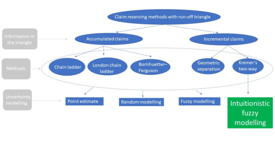
1. Introduction

1.1. Preliminary Considerations

The process of claim reserving is at the core of the financial management of general insurance organizations. It determines what is held on the balance sheet for claims that are not yet settled, affects the premiums that are charged, and impacts the capital that is held to support the solvency of the organization [1]. For claim reserving methods, the literature commonly differentiates between deterministic and stochastic methods [2]. Deterministic methods provide a point estimate for reserves, i.e., the most reliable value. However, stochastic reserving methods provide both a point estimate and a quantification of the variability around the fair value [2].

The relevance of reliable estimations of the fair value of provisions, as well as of their variability from available information, is of great interest in actuarial judgement, which must determine the final value of the provisions [3]. The estimation of reserves must be prudent and cover possible unfavourable deviations from their expected value; however, it should not be excessive [4].

In the actuarial field, fuzzy set theory (FST) has been used to model situations that require a great deal of actuarial subjective judgement and problems for which the information available is scarce or vague. Therefore, Refs. [5,6,7] proposed the use of fuzzy numbers (FNs) to model uncertainty in actuarial parameters. This imprecision is undoubtedly present in the adjustment of claim provisions. Therefore, the available data may be subject to vagueness and imprecision [8]. Moreover, it is not advisable to use a wide database to calculate claim reserves; data too far from the present can lead to unrealistic estimates. For example, if claims are related to bodily injuries, future losses for the company will depend on the growth of the wage index (which will be used to determine the amount of indemnification due), changes in court practices, and public awareness of liability matters [9].

These reasons explain the contributions, which are indicated in Table 1, in which reserves were calculated using FST tools. Therefore, in addition to deterministic and stochastic claim reserving, there is a third approach that we call fuzzy claim reserving. Fuzzy methods, such as stochastic methods, seek to quantify, apart from the most likely value of claims provisions, possible fluctuation bands around the most reliable value of these reserves [3]. In these studies, the imprecision of the parameters that allow for the calculation of claim reserves is modelled through fuzzy numbers (FNs). In these contributions, FNs must be interpreted as quantifications of epistemic uncertainty, capturing vague or incomplete information about the value of the parameter of interest [10].

In general, as shown in Table 1 and as with stochastic methods, fuzzy methods are grounded from a deterministic framework. While in stochastic approaches, the analytical schema adapts to the assumption of the randomness of the parameters, fuzzy approaches adapt them to the hypothesis that the parameters governing the evolution of claims are possibility distributions. The most commonly used groundworks in fuzzy claim reserving are the chain ladder [11,12] and the geometric separation method [13], with examples shown in [14,15]. The fuzzy literature has also adopted two-way ANOVA [16], two-way ANCOVA [17], and a Poisson generalized linear model framework [18,19].

Table 1 shows that in most studies, the parameters of the reserving framework are adjusted using fuzzy regression techniques. In this sense, two streams of fuzzy regression methods should be differentiated: possibilistic regression, which we call the minimum fuzziness principle (MFP), and minimization of distances, such as fuzzy least squares (FLS) [20]. Among the MFP models, we first highlight the studies by Tanaka [21] and Tanaka and Ishibuchi [22], which assume symmetry in the parameters and have been applied in a claim reserving context [11,15]. Secondly, we outline the methodology of Ishibuchi and Nii [23], which combines minimum-square regression to adjust the values of maximum reliability and the minimum fuzziness principle. Some contributions to fuzzy loss reserving using this approach are found in [16,17,18]. In terms of contributions to fuzzy least squares in claim reserving, we can outline the studies of [14,15,19].

Table 1 shows that the most common shape of parameters in the fuzzy claim reserving literature is triangular fuzzy numbers (TFNs). In some contributions, these methods do not have restrictions regarding symmetry [16,17,18,19]. However, the hypothesis of symmetry is very common [11,12,14,24,25].

Table 1. Panoramic view of fuzzy claim reserving.

Paper	Focus	Adjusting Method	Shape
Andrés-Sánchez [4]	Detrends link ratios with a fuzzy Hoerl curve	MFP	TFNs
Andrés-Sánchez and Terceño [11]	Extends London chain ladder method to fuzzy development factors	MFP	STFNs
Heberle and Thomas [12]	Extends the conventional chain ladder method to the use of fuzzy development factors	Heuristically	STFNs
Kim and Kim [17]	Extends ANCOVA two-way framework to the presence of possibilistic parameters	MFP	TFNs
Apaydin and Baser [14]	Extends Taylor’s geometric separation method to possibilistic parameters	FLS	STFNs
Yan et al. [15]	Uses Taylor’s geometric separation method to possibilistic parameters	FLS and MFP	STFNs
Andrés-Sánchez [16]	Extends ANOVA two-way framework to the presence of possibilistic parameters	MFP	TFNs
Woundjiagué et al. [18]	Extends Poisson framework for claim reserving	FLS	TFNs
Woundjiagué et al. [19]	Extends Poisson framework for claim reserving	MFP	TFNs
Heberle and Thomas [24]	Extends the Bornhuetter–Ferguson method to the use of fuzzy development factors	Heuristically	STFNs
Bastos et al. [25]	Extends chain ladder method to the use of Gaussian possibility distributions	Heuristically	GFNs
Andrés-Sánchez [26]	Extends Taylor’s geometric separation method to possibilistic parameters	MFP	TFNs
Baser and Apaydin, [27]	Extends London chain ladder to the use of fuzzy numbers	FLS	STFNs
Andrés-Sánchez [28]	Obtains closed expressions for the point value from estimated of ANOVA two way	MFP	TFNs
Yan et al. [29]	Extends double chain ladder (number of claims and accumulated claims)	Heuristically	TFNs

Note: MFP stands for the minimum fuzziness principle, and FLS stands for fuzzy least squares. TFNs stands for triangular fuzzy numbers, STFNs for symmetrical triangular fuzzy numbers, and GFN for Gaussian fuzzy numbers.

Table 1. Panoramic view of fuzzy claim reserving.

Paper	Focus	Adjusting Method	Shape
Andrés-Sánchez [4]	Detrends link ratios with a fuzzy Hoerl curve	MFP	TFNs
Andrés-Sánchez and Terceño [11]	Extends London chain ladder method to fuzzy development factors	MFP	STFNs
Heberle and Thomas [12]	Extends the conventional chain ladder method to the use of fuzzy development factors	Heuristically	STFNs
Kim and Kim [17]	Extends ANCOVA two-way framework to the presence of possibilistic parameters	MFP	TFNs
Apaydin and Baser [14]	Extends Taylor’s geometric separation method to possibilistic parameters	FLS	STFNs
Yan et al. [15]	Uses Taylor’s geometric separation method to possibilistic parameters	FLS and MFP	STFNs
Andrés-Sánchez [16]	Extends ANOVA two-way framework to the presence of possibilistic parameters	MFP	TFNs
Woundjiagué et al. [18]	Extends Poisson framework for claim reserving	FLS	TFNs
Woundjiagué et al. [19]	Extends Poisson framework for claim reserving	MFP	TFNs
Heberle and Thomas [24]	Extends the Bornhuetter–Ferguson method to the use of fuzzy development factors	Heuristically	STFNs
Bastos et al. [25]	Extends chain ladder method to the use of Gaussian possibility distributions	Heuristically	GFNs
Andrés-Sánchez [26]	Extends Taylor’s geometric separation method to possibilistic parameters	MFP	TFNs
Baser and Apaydin, [27]	Extends London chain ladder to the use of fuzzy numbers	FLS	STFNs
Andrés-Sánchez [28]	Obtains closed expressions for the point value from estimated of ANOVA two way	MFP	TFNs
Yan et al. [29]	Extends double chain ladder (number of claims and accumulated claims)	Heuristically	TFNs

Note: MFP stands for the minimum fuzziness principle, and FLS stands for fuzzy least squares. TFNs stands for triangular fuzzy numbers, STFNs for symmetrical triangular fuzzy numbers, and GFN for Gaussian fuzzy numbers.

1.2. Using Intuitionistic Fuzzy Numbers to Adjust Claim Reserves

In the review of fuzzy claim reserving conducted in the previous subsection, fuzzy uncertainty was modelled using type-1 fuzzy numbers but not with higher-order fuzzy sets such as type-2 fuzzy numbers or, as in this paper, intuitionistic fuzzy numbers (IFNs). This kind of fuzzy modelling allows more nuances to be captured in the information than simple FNs.

The concept of intuitionistic fuzzy numbers (IFNs) is a tool in the theory of intuitionistic fuzzy sets [30,31] that allows the quantification of uncertain quantities by extending the concept of FNs [32]. IFNs facilitate the inclusion of bipolar information along with epistemic uncertainty in the quantification of parameters of interest. This involves using both positive information about the values that the parameter of interest can take and negative information about the values that the parameter actually cannot take [10].

Bipolarity does not introduce additional uncertainty [10] but provides new information. In the case of IFNs, this entails adding an estimate of values that, with certainty, should be excluded, thus complementing information about the believed possible values of a parameter.

1.3. Using Intuitionistic Fuzzy Numbers to Adjust Claim Reserves

The application of IFN parameters in financial and actuarial issues is significantly scarcer than that of conventional fuzzy numbers. Relevant applications include capital budgeting [33,34,35,36], option pricing [37], and real option pricing [38,39]. Similarly, [40] uses intuitionistic fuzzy values to address environmental risk analysis.

Therefore, we think that the introduction of IFN in the quantification of claims provisions is of interest. On the one hand, this analysis allows for expanding the applications of intuitionistic fuzzy numbers in a scarcely explored field, such as insurance. This approach is novel from both the perspectives of intuitionistic mathematics and actuarial mathematics. Moreover, the use of IFNs allows for the introduction of more information into the analysis than the utilization of confidence intervals or simply fuzzy numbers. While confidence intervals and FNs only capture possible values of the parameters of interest, the use of IFN parameters allows for using estimates of values that are deemed impossible. If such information exists, the use of FNs does not allow for introducing it into the analysis. In cases where information about such unreliable values does not exist, IFNs are simply FNs. Therefore, the introduction of IFNs allows for generalizing the developments made with FNs.

Building upon the reflections presented in this introduction, this paper makes two contributions:

• Parvati et al. [41] generalized the regression model [21,22], and thus modelled the coefficients as symmetric TIFNs. Drawing inspiration from [41], our study extends the fuzzy regression method [23] to the use of TIFNs, which, on the other hand, are not necessarily symmetric.
• We apply the intuitionistic extension to the regression model [23] to adjust claim reserves under the ANOVA two-way schema [42,43].

The remainder of this paper is organized as follows. The next section introduces the fundamentals of intuitionistic fuzzy numbers and their arithmetic operations. The third section introduces the intuitionistic generalization of the regression model [23]. The fourth section introduces the methodologies that will be used as benchmarks, the chain ladder model in its deterministic and random versions, and two-way ANOVA [42,43]. This section also develops the intuitionistic version of two-way ANOVA. In the fifth section, we compare the proposed intuitionistic methodology with benchmark methods in a numerical application. The study concludes by highlighting the main results and suggesting further research.

2. Intuitionistic Fuzzy Numbers

2.1. Fuzzy Numbers and Intuitionistic Fuzzy Numbers

Definition 1.

A fuzzy set (FS) in a referential set $X$, $\ddot{A}$ is defined as [44]:

$$\ddot{A}=\left\{〈x,{\mu }_A\left(x\right)〉, x\in X\right\},$$

where ${\mu }_A:X⟶\left[0,1\right]$ is the so-called membership function.

Definition 2.

The fuzzy set $\ddot{A}$ can be represented through level sets or $\alpha$-cuts, $A_{\alpha }$ [44]:

$$A_{\alpha }=\left\{x|{\mu }_A\left(x\right)\ge \alpha , 0<\alpha \le 1\right\}.$$

Definition 3.

A fuzzy number (FN), $\ddot{A}$, is a fuzzy subset of the real line [45] such that the membership function ${\mu }_A\left(x\right)$ is an upper semicontinuous function that accomplishes:

 i.

is normal, i.e., $\exists x|{\mu }_A\left(x\right)=1.$

ii. 

is convex, i.e.,

$$\forall x_1,x_2\in \mathbb{R},0\le \lambda \le 1,{\mu }_A\left({\lambda x}_1,\left(1-\lambda \right)x_2\right)\ge \min \left({\mu }_A\left(x_1\right),{\mu }_A\left(x_2\right)\right).$$

Remark 1.

As a consequence, the α-cuts of $\ddot{A}$ and $A_{\alpha }$ are confidence intervals:

$$A_{\alpha }=\left\{x|{\mu }_A\left(x\right)\ge \alpha , 0<\alpha \le 1\right\}=\left[{\underset{\_}{A}}_{\alpha }, {\overline{A}}_{\alpha }\right],$$

where ${\underset{\_}{A}}_{\alpha }$ is an increasing function of $\alpha$ and ${\overline{A}}_{\alpha }$ is a decreasing function.

Remark 2.

The membership function of $\ddot{A}{, \mu }_A\left(x\right)$ is also called the distribution function.

Definition 4.

A triangular fuzzy number (TFN) can be represented by the triplet $\ddot{A}=\left(A,l_A{,r}_A\right)$, $l_A, r_A\ge 0$. Then, the membership function is as follows:

$${\mu }_A\left(x\right)=\left\{\begin{array}{cc}\frac{x-A+l_A}{l_A}& A-l_A<x<A\\ \frac{A+r_A-x}{r_A}& A<x<A+r_A\\ \begin{array}{c}1\\ 0\end{array}& \begin{array}{c}x=A\\ \mathrm{o}\mathrm{t}\mathrm{h}\mathrm{e}\mathrm{r}\mathrm{w}\mathrm{i}\mathrm{s}\mathrm{e}\end{array}\end{array}\right.,$$

being the α-cut representation:

$$A_{\alpha }=\left[{\underset{\_}{A}}_{\alpha }, {\overline{A}}_{\alpha }\right]=\left[A-l_A\left(1-\alpha \right),A+r_A\left(1-\alpha \right)\right],\hspace{1em}0\le \alpha \le 1.$$

Fuzzy set theory commonly represents imprecise quantities and parameters using fuzzy numbers (FNs) [45]. Specifically, TFNs are very common in practical applications within fuzzy set theory since the grading of the membership level is performed linearly, which is reasonable because it applies the principle of parsimony when dealing with vague information [46].

Definition 5.

The intuitionistic fuzzy set (IFS) $\tilde{A}$ defined in a referential set $X$ is [30]:

$$\tilde{A}=\left\{〈x,{\mu }_A\left(x\right),v_A\left(x\right)〉, x\in X\right\},$$

where ${\mu }_A:X⟶\left[0,1\right]$ measures the membership of $x$ in $\tilde{A}$, and $v_A:X⟶\left[0,1\right]$ is nonmembership. These functions must accomplish the following:

$$0\le {\mu }_A\left(x\right)+v_A\left(x\right)\le 1.$$

Remark 3.

Note that ${\mu }_A\left(x\right)+v_A\left(x\right)=1$ is not necessarily true, that is, an element $x$ is allowed to belong to $\tilde{A}$ and its complement with a degree of hesitancy, $h_A\left(x\right)$, which is:

$$h_A\left(x\right)=1-{\mu }_A\left(x\right)-v_A\left(x\right).$$

Remark 4.

An IFS generalizes the concept of an FS such that if $h_A\left(x\right)=0 \forall x$, $\tilde{A}$ is a conventional FS.

Definition 6.

An IFN can be expressed using $〈\alpha ,\beta 〉$-levels or $〈\alpha ,\beta 〉$-cuts, $A_{〈\alpha ,\beta 〉}$, [30]:

$$A_{〈\alpha ,\beta 〉}=\left\{x|{\mu }_A\left(x\right)\ge \alpha , v_A\left(x\right)\le \beta ,0\le \alpha +\beta \le 1,\alpha ,\beta \in \left[0,1\right]\right\}.$$

Remark 5.

$A_{〈\alpha ,\beta 〉}$ can be decoupled into two level sets [47]:

$$A_{\alpha }=\left\{{x|\mu }_A\left(x\right)\ge \alpha \right\} and A_{\beta }^{*}=\left\{x|v_A\left(x\right)\le \beta \right\},$$

in such a way that

$$A_{〈\alpha ,\mathsf{\beta }〉}=〈A_{\alpha }=\left\{{x|\mu }_A\left(x\right)\ge \alpha \right\},A_{\beta }^{\mathrm{*}}=\left\{x|v_A\left(x\right)\le \beta \right\},0\le \mathsf{\alpha }+\beta \le 1,\mathsf{\alpha },\beta \in \left[0,1\right]〉.$$

Definition 7.

An intuitionistic fuzzy number (IFN) is an IFS defined for real numbers [34], such that the membership function ${\mu }_A\left(x\right)$ and the nonmembership function $v_A\left(x\right)$ are upper semicontinuous functions that accomplish the following:

  i. 

It is normal, i.e., $\exists x|{\mu }_A\left(x\right)=1\Rightarrow v_A\left(x\right)=h_A\left(x\right)=0.$

 ii.

${\mu }_A\left(x\right)$ is convex,

$$\forall x_1,x_2\in \mathbb{R},0\le \lambda \le 1,{\mu }_A\left({\lambda x}_1,\left(1-\lambda \right)x_2\right)\ge \min \left({\mu }_A\left(x_1\right),{\mu }_A\left(x_2\right)\right),$$

iii. 

and $v_A\left(x\right)$ is concave:

$$\forall x_1,x_2\in \mathbb{R},0\le \lambda \le 1,v_A\left({\lambda x}_1,\left(1-\lambda \right)x_2\right)\le \max \left(v_A\left(x_1\right),v_A\left(x_2\right)\right).$$

Remark 6.

The $〈\alpha ,\beta 〉$-cuts of $\tilde{A}$ and $A_{〈\alpha ,\beta 〉}$ can be decoupled as:

$$A_{\alpha }=\left\{{x|\mu }_A\left(x\right)\ge \alpha \right\}=\left[{\underset{\_}{A}}_{\alpha }, {\overline{A}}_{\alpha }\right] and A_{\beta }^{*}=\left\{v_A\left(x\right)\le \beta \right\}=\left[{\underset{\_}{A^{*}}}_{\beta },{\overline{A^{*}}}_{\beta }\right], 0\le \alpha +\beta \le 1, \alpha ,\beta \in (0,1),$$

where ${\underset{\_}{A}}_{\alpha }$ $\left({\overline{A}}_{\alpha }\right)$ is an increasing (decreasing) function of $\alpha$ and ${\underset{\_}{A^{*}}}_{\beta }$ $\left({\overline{A^{*}}}_{\beta }\right)$ decreases (increases) with respect to $\beta$.

Remark 7.

Thus, an $〈\alpha ,\beta 〉$-level of $A_{〈\alpha ,\beta 〉}$ can be represented:

$$A_{〈\alpha ,\beta 〉}=〈A_{\alpha }=\left[{\underset{\_}{A}}_{\alpha },{\overline{A}}_{\alpha }\right],{A^{*}}_{\beta }=\left[{\underset{\_}{A^{*}}}_{\beta },{\overline{A^{*}}}_{\beta }\right],0\le \alpha +\beta \le 1,\alpha ,\beta \in (0,1) 〉.$$

An IFN is an imprecise quantity that must be quantified by a real number. If nonmembership is established as $v_A\left(x\right)=1-{\mu }_A\left(x\right) \forall x$, then $\tilde{A}$ is an FN.

Remark 8.

In an IFN, ${\mu }_A\left(x\right)$ is also known as the lower possibility distribution function of the quantity of interest A, and ${\mu }_{A^{*}}\left(x\right)=1-v_A\left(x\right)$ is the upper distribution function of the uncertain quantity [32].

The membership functions ${\mathsf{\mu }}_{{\mathrm{A}}^{\mathrm{*}}}\left(\mathrm{x}\right)$ and ${\mathsf{\mu }}_{\mathrm{A}}\left(\mathrm{x}\right)$ can be interpreted as bipolar possibility distribution measurements in such a way that ${\mathsf{\mu }}_{{\mathrm{A}}^{\mathrm{*}}}\left(\mathrm{x}\right)$ accounts for the potential possibility and ${\mathsf{\mu }}_{\mathrm{A}}\left(\mathrm{x}\right)$ accounts for the real possibility of $\mathrm{A}$ being $\mathrm{x}$ [10].

Definition 8.

A triangular intuitionistic fuzzy number (TIFN) can be denoted as $\tilde{A}=\left(A,l_A{,l_A^{*},r}_A,r_A^{*} \right)$, with membership and nonmembership functions [41]:

$${\mu }_A\left(x\right)=\left\{\begin{array}{cc}\frac{x-A+l_A}{l_A}& A-l_A<x<A\\ \frac{A+r_A-x}{r_A}& A<x<A+r_A\\ \begin{array}{c}1\\ 0\end{array}& \begin{array}{c}x=A\\ otherwise\end{array}\end{array}\right.,$$

(1a)

and

$${\upsilon }_A\left(x\right)=\left\{\begin{array}{cc}\frac{A-x}{l_A^{*}}& A-l_A^{*}<x<A\\ \frac{x-A}{r_A^{*}}& A<x<A+r_A^{*}\\ \begin{array}{c}0\\ 1\end{array}& \begin{array}{c}x=A\\ \mathrm{o}\mathrm{t}\mathrm{h}\mathrm{e}\mathrm{r}\mathrm{w}\mathrm{i}\mathrm{s}\mathrm{e}\end{array}\end{array}\right.,$$

(1b)

where $l_A\le l_A^{*}$ and $r_A\le r_A^{*}$. Figure 1 depicts the shape of a TIFN and the relationship between the embedded functions, ${\mu }_A\left(x\right),$ $v_A\left(x\right)$, ${\mu }_{A^{*}}\left(x\right)$ and $h_A\left(x\right).$

Remark 9.

The level sets $A_{〈\alpha ,\beta 〉},$ of a TIFN can be decoupled into:

$$A_{\alpha }=\left[{\underset{\_}{A}}_{\alpha }, {\overline{A}}_{\alpha }\right]=\left[A-l_A\left(1-\alpha \right),A+r_A\left(1-\alpha \right)\right],$$

(1c)

$${A^{*}}_{\beta }=\left[{\underset{\_}{A^{*}}}_{\beta },{\overline{A^{*}}}_{\beta }\right]=\left[A-l_A^{*}\beta ,A+r_A^{*}\beta \right].$$

(1d)

Thus, TIFNs are an extension of TFNs, such that if $l_A=l_A^{*}$ and $r_A=r_A^{*}$, we deal with a conventional TFN [48]. Triangular uncertain parameters are commonly considered in practical applications involving intuitionistic modelling [34,48,49,50,51]. The argument put forward in [46], based on the application of the parsimony principle for the use of TFNs, can be extended to the use of TIFNs.

A TIFN adapts very naturally to the way humans make estimations by incorporating more nuances than are necessary to fit a TFN. Thus, $A$ represents the scenario with the maximum reliability. Moreover, whereas $A-l_A$ and $A-l_A^{*}$ are two extreme lower-case scenarios, $A+r_A$ and $A+r_A^{*}$ are two extreme upper-case scenarios. $A-l_A$ is considerably lower than the central value, and $A-l_A^{*}$ is exceptionally low compared to the possible values of the parameter. For example, in the context of a random variable, the first scenario could be a reasonably small percentile (e.g., the 5th percentile), and the second could be a virtually impossible value (e.g., the 0.1 percentile). If ${A-l}_A^{*}<x\le A-l_A, {\mu }_A\left(x\right)=$0, we do not assign a likelihood to parameter $\tilde{A}$ taking the value $x$ but rather express some level of doubt about its nonmembership, $h_A\left(x\right)>0$, because $v_A\left(x\right)<1$.

Of course, $A+r_{\mathrm{A}}$, which can be assimilated to a relatively high percentile of a random variable (e.g., the 95th percentile) must be interpreted in a similar way. In contrast, $A+r_A^{*}$ is potentially an extremely high value (e.g., 99.5th percentile).

Note that TIFNs allow modelling estimations of a parameter that, while its knowledge may also be vague and imprecise, contains more nuances than an FN. For instance, a statement such as “An adequate interest rate to fit discounted reserves is approximately 3%, ranging from 2.5% to 4%. However, that a value must not be lower than 2% or higher than 5%” could be quantified as the TIFN (3%, 0.5%, 0.5%, 1%, 1%).

2.2. Intuitionistic Fuzzy Number Arithmetic

In the Introduction, we reviewed various approaches that fuzzy research has provided for estimating claim reserves using fuzzy logic. Ultimately, obtaining estimates for outstanding claims at different time points will require the evaluation of parameter functions whose values are fuzzy. This issue necessitates the application of Zadeh’s extension principle with max–min operators, which are typically implemented through the functional analysis of alpha-level sets.

The results of [52] allow the evaluation of functions with fuzzy estimates of variables through alpha-cuts developed in [53,54,55] to be generalized to IFN arithmetic. As far as we are concerned, we will evaluate continuous and differentiable functions, $y=f\left(x_1,x_2,\dots ,x_n\right)$, such that the values of the input variables are given the means of IFNs ${\tilde{A}}_{\left(i\right)}, i=\mathrm{1,2},\dots ,n$. This generates IFN $\tilde{B}$, $\tilde{B}=f\left({\tilde{A}}_{\left(1\right)},{\tilde{A}}_{\left(2\right)},\dots ,{\tilde{A}}_{\left(n\right)}\right)$. The use of the generalized Zadeh’s principle by using the min–norm and max–conorm allows us to state the membership and nonmembership of $\tilde{B}$ as [41,52]:

$${\mu }_B\left(y\right)=\underset{y=f\left(x_1,x_2,\dots ,x_n\right)}{\max }\min \left\{{\mu }_{A_{\left(1\right)}}\left(x_1\right),{\mu }_{A_{\left(2\right)}}\left(x_2\right),\dots ,{\mu }_{A_{\left(n\right)}}\left(x_n\right)\right\},$$

$$v_B\left(y\right)=\underset{y=f\left(x_1,x_2,\dots ,x_n\right)}{\min }\max \left\{v_{A_{\left(1\right)}}\left(x_1\right),v_{A_{\left(2\right)}}\left(x_2\right),\dots ,v_{A_{\left(n\right)}}\left(x_n\right)\right\}.$$

Therefore, if ${\tilde{A}}_{\left(i\right)}, i=\mathrm{1,2},\dots ,n$ are FNs, it is only necessary to obtain ${\mu }_B\left(y\right)$ using the usual max–min principle.

The evaluation of the functions of FNs such as TFNs is often performed through α-level sets [54,55]. Similarly, the value of the intuitionistic fuzzy number $\tilde{B}=f\left({\tilde{A}}_{\left(1\right)},{\tilde{A}}_{\left(2\right)},\dots ,{\tilde{A}}_{\left(n\right)}\right)$ is obtained by means of its $〈\alpha ,\beta 〉-$cuts, $B_{〈\alpha ,\beta 〉}$, instead of by evaluating ${\mu }_B\left(y\right)$ and $v_B\left(y\right)$. Thus, to obtain $B_{〈\alpha ,\beta 〉}$, we must implement $f\left(x_1,x_2,\dots ,x_n\right)$ from the $〈\alpha ,\beta 〉-$cuts of ${\tilde{A}}_{\left(i\right)}$, ${A_{\left(i\right)}}_{〈\alpha ,\beta 〉}, i=\mathrm{1,2},\dots ,n$:

$$B_{〈\alpha ,\beta 〉}=f\left({A_{\left(1\right)}}_{〈\alpha ,\beta 〉},{A_{\left(2\right)}}_{〈\alpha ,\beta 〉},\dots ,{A_{\left(n\right)}}_{〈\alpha ,\beta 〉}\right),$$

and given that ${A_{\left(i\right)}}_{〈\alpha ,\beta 〉}$ is decoupled in ${A_{\left(i\right)}}_{\alpha }$ and ${A_{\left(i\right)}^{*}}_{\alpha }$ (see Remark 7) and that $f$ is continuous, $B_{〈\alpha ,\beta 〉}$ can also be decoupled in $B_{\alpha }=\left[{\underset{\_}{B}}_{\alpha },{\overline{B}}_{\alpha }\right]$ and ${B^{\mathrm{*}}}_{\beta }=\left[{\underset{\_}{B^{\mathrm{*}}}}_{\beta },{\overline{B^{\mathrm{*}}}}_{\beta }\right]$. According to [54,55], when $f$ monotonically increases with respect to $x_i, i=\mathrm{1,2},\dots m$ and monotonically decreases in $x_i, i=m+1,m+2,\dots ,n$,$m\le n$, $B_{\alpha }$ is:

$${\underset{\_}{B}}_{\alpha }=f\left({\underset{\_}{A_{\left(1\right)}}}_{\alpha },{\underset{\_}{A_{\left(2\right)}}}_{\alpha },\dots ,{\underset{\_}{A_{\left(m\right)}}}_{\alpha },{\overline{A_{\left(m+1\right)}}}_{\alpha },\dots {,\overline{A_{\left(n\right)}}}_{\alpha }\right),$$

(2a)

$${\overline{B}}_{\alpha }=f\left({\overline{A_{\left(1\right)}}}_{\alpha },{\overline{A_{\left(2\right)}}}_{\alpha },\dots ,{\overline{A_{\left(m\right)}}}_{\alpha },{\underset{\_}{A_{\left(m+1\right)}}}_{\alpha },\dots {,\underset{\_}{A_{\left(n\right)}}}_{\alpha }\right).$$

(2b)

By comparison, the β-cuts of ${B^{*}}_{\beta }$ are

$${\underset{\_}{B^{\mathrm{*}}}}_{\beta }=f\left({\underset{\_}{A_{\left(1\right)}^{\mathrm{*}}}}_{\beta },{\underset{\_}{A_{\left(2\right)}^{\mathrm{*}}}}_{\beta },\dots ,{\underset{\_}{A_{\left(m\right)}^{\mathrm{*}}}}_{\beta },{\overline{A_{\left(m+1\right)}^{\mathrm{*}}}}_{\beta },\dots ,{\overline{A_{\left(n\right)}^{\mathrm{*}}}}_{\beta }\right),$$

(2c)

$${\overline{B^{\mathrm{*}}}}_{\beta }=f\left({\overline{A_{\left(1\right)}^{\mathrm{*}}}}_{\beta },{\overline{A_{\left(2\right)}^{\mathrm{*}}}}_{\beta },\dots ,\overline{{A_{\left(m\right)}^{\mathrm{*}}}_{\beta }},{\underset{\_}{A_{(m+1)}^{\mathrm{*}}}}_{\beta },\dots {\underset{\_}{{,A}_{\left(n\right)}^{\mathrm{*}}}}_{\beta }\right).$$

(2d)

The linear combination of TIFNs is also a TIFN. Therefore, let us have a linear operation $\tilde{B}=\sum _{i=1}^n{\lambda }_i{\tilde{A}}_{\left(i\right)},$ where ${\lambda }_iϵ\mathbb{R}$ and ${\tilde{A}}_{\left(i\right)}=\left(A_{\left(i\right)},l_{A_{\left(i\right)}}{,l_{A_{\left(i\right)}}^{\mathrm{*}},r}_{A_{\left(i\right)}},r_{A_{\left(i\right)}}^{\mathrm{*}}\right),i=\mathrm{1,2},\dots ,n.$ Therefore, $\tilde{B}=\left(B,l_B{,l_B^{\mathrm{*}},r}_B,r_B^{\mathrm{*}}\right)$, where [41]

$$B=\sum _{i=1}^n{\lambda }_i{A}_{\left(i\right)},$$

(3a)

$${ l}_B=\sum _{i|{\lambda }_i\ge 0}{\lambda }_i·l_{A_{\left(i\right)}}+\sum _{i|{\lambda }_i<0}\left|{\lambda }_i\right|·r_{A_{\left(i\right)}},{ l}_B^{*}=\sum _{i|{\lambda }_i\ge 0}{\lambda }_i·l_{A_{\left(i\right)}}^{*}+\sum _{i|{\lambda }_i<0}\left|{\lambda }_i\right|·r_{A_{\left(i\right)}}^{*} ,$$

(3b)

$${ r}_B=\sum _{i|{\lambda }_i\ge 0}{\lambda }_i·r_{A_{\left(i\right)}}+\sum _{i|{\lambda }_i<0}\left|{\lambda }_i\right|·l_{A_{\left(i\right)}},{ r}_B^{*}=\sum _{i|{\lambda }_i\ge 0}{\lambda }_i·r_{A_{\left(i\right)}}^{*}+\sum _{i|{\lambda }_i<0}\left|{\lambda }_i\right|·l_{A_{\left(i\right)}}^{*}.$$

(3c)

Given that the evaluation of nonlinear functions using TFNs does not produce a TIFN, it can also be generalized to TIFNs. Despite this limitation, [46] argues that linear shapes often offer an effective solution to practical issues in the majority of cases. It is well known that there are many financial functions that, despite not being linear, when they are evaluated, the result is accurately approximated by a TFN that conserves the same support (the 0-cut) and core (the 1-cut). In the actuarial field, this has been proposed for the estimation of claim reserves [11,12,17,24], the final value of a pension plan [56], asymptotic probabilities of the number of claims in a bonus-malus system [57], or the price of life settlements [58]. Following the same philosophy, [33] postulates that the net present value function, when cash flows and discount rates are estimated using TIFNs, can be approximated through a TIFN with the same <0,1>-cut and <1,0>-cut. Therefore, in this study, when the initial data are estimated by TIFNs ${\tilde{A}}_{\left(i\right)}, i=1,2,\dots ,n$, the approximate TIFN $\widetilde{B^T}\approx \tilde{B}=f\left({\tilde{A}}_{\left(1\right)},{\tilde{A}}_{\left(2\right)},\dots ,{\tilde{A}}_{\left(n\right)}\right),$ is considered:

$$\widetilde{B^T}=\left(B,{ l}_B{,{ l}_B^{*}, r}_B,{ r}_B^{*} \right)=\left({{\underset{\_}{B}}_1=\overline{B}}_1,{\underset{\_}{B}}_1-{\underset{\_}{B}}_0,{\underset{\_}{B^{\mathrm{*}}}}_1-{\underset{\_}{B^{\mathrm{*}}}}_0,{\overline{B}}_0-{\overline{B}}_1,{\overline{B^{\mathrm{*}}}}_0-{\overline{B^{\mathrm{*}}}}_1\right),$$

(4)

By comparison with the error measurement in the triangular approximation of fuzzy numbers [58], the quality of the relative error measurement in the bounds of $B_{〈\alpha ,\beta 〉}$ calculated with (2a–d) by those of its triangular approximation, (4), $B_{〈\alpha ,\beta 〉}^T$ in $B_{\alpha }=\left[{\underset{\_}{B}}_{\alpha },{\overline{B}}_{\alpha }\right]$ are:

$${\underset{\_}{\epsilon }}_{\alpha }=\frac{\left|{\underset{\_}{B}}_{\alpha }-{\underset{\_}{B^T}}_{\alpha }\right|}{{\underset{\_}{B}}_{\alpha }},{\overline{\epsilon }}_{\alpha }=\frac{\left|{\overline{B}}_{\alpha }-{\overline{B^T}}_{\alpha }\right|}{{\overline{B}}_{\alpha }},{\underset{\_}{{\epsilon }^{\mathrm{*}}}}_{\beta }=\frac{\left|{\underset{\_}{B^{\mathrm{*}}}}_{\beta }-{\underset{\_}{B^{T\mathrm{*}}}}_{\beta }\right|}{{\underset{\_}{B^{\mathrm{*}}}}_{\beta }},{\overline{{\epsilon }^{\mathrm{*}}}}_{\beta }=\frac{\left|{\overline{B^{\mathrm{*}}}}_{\beta }-{\overline{B^{T\mathrm{*}}}}_{\beta }\right|}{{\overline{B^{\mathrm{*}}}}_{\beta }}.$$

(5)

The use of Equation (5) allows us to assess the goodness of fit of the linear approximation in numerical applications, which requires only evaluating five scenarios in (4) compared to the exact $〈\alpha ,\beta 〉$-cuts that require the calculation of (3a–d) for the established $〈\alpha ,\beta 〉$ pairs.

3. Intuitionistic Linear Regression with the Minimum Fuzziness Principle and Asymmetric Coefficients

Within fuzzy regression models, we can identify two major families. The first group consists of possibilistic regressions that are also referred to as minimum fuzziness principle (MFP) regressions. Some examples are [21,22,23], which fit parameters by minimizing the fuzziness of the system, subject to the condition that the adjusted function must include the observations [20]. Secondly, we can outline the methodology based on the minimization of the distance between observations and estimates. A clear example in this regard is the method known as fuzzy least squares [20]. Our approach should be understood within this first stream.

Parvati et al. [41] generalized the regression model [21,22]. Thus, given that [21,22] modelled the coefficients as symmetric TFNs, [41] assumed that these coefficients were symmetric TIFNs. Drawing inspiration from [41], our study extends the fuzzy regression method [23] to the use of TIFNs. In contrast to [41], we do not require the coefficients to be symmetrical. The advantage of this approach is that we can capture the possibility of asymmetry in the system, as the adjusted coefficients will generally be nonsymmetric. The disadvantage is that, while in [41], the parameters are adjusted by solving a single minimization program, our method requires the sequential application of ordinary least squares and the resolution of a linear program similar to that of [41].

We start with the assumption that the system is adjusted and has an outcome variable dependent on m crisp input variables, $x_i$, i = 0, 1, 2…, m, where $x_0=1$ and $x_iϵ\mathbb{R}$, i = 1, 2,…, n. The outcome is a linear function of intuitionistic coefficients ${\tilde{A}}_{\left(i\right)}=\left(A_{\left(i\right)},l_{A_{\left(i\right)}}{,l_{A_{\left(i\right)}}^{*},r}_{A_{\left(i\right)}},r_{A_{\left(i\right)}}^{*} \right), i=0,1,\dots ,m$ and, therefore, a TIFN $\tilde{Y}=\left(Y,l_Y{,l_Y^{*},r}_Y,r_Y^{*} \right)$. This is obtained by considering that the observations of the input variables $x_i, i=0,1,\dots ,n,$ are the scalars in (3a–c). Thus, Equation (3) in [41] is extended to nonsymmetrical TIFNs as follows:

$$Y=\sum _{j=0}^m{A}_{\left(i\right)}{x}_i,$$

(6a)

$${ l}_Y=\sum _{i|x_i\ge 0}{l}_{A_{\left(i\right)}}{x}_i+\sum _{i|x_i<0}{r}_{A_{\left(i\right)}}\left|x_i\right|,{ l}_Y^{*}=\sum _{i|x_i\ge 0}{l}_{A_{\left(i\right)}}^{*}{x}_i+\sum _{i|x_i<0}{r}_{A_{\left(i\right)}}^{*}\left|x_i\right| ,$$

(6b)

$${ r}_Y=\sum _{i|x_i\ge 0}{r}_{A_{\left(i\right)}}{x}_i+\sum _{i|x_i<0}{l}_{A_{\left(i\right)}}\left|x_i\right|,{ r}_Y^{*}=\sum _{i|x_i\ge 0}{r}_{A_{\left(i\right)}}^{*}{x}_i+\sum _{i|x_i<0}{l}_{A_{\left(i\right)}}^{*}\left|x_i\right| .$$

(6c)

Moreover, both the observations of the input and output variables are crisp. This is a common circumstance in fuzzy regression models, and [23,41] also assume such a situation. Thus, for the j-th observation, the outcome is the crisp number $y_j$, generated by the crisp incomes $(1,x_{1j}, x_{2j},\dots ,x_{ij},\dots ,x_{im})$. Therefore, $y_j$ is a possible value of a TIFN $\widetilde{Y_j}=\left(Y_j,l_{Y_j}{,l_{Y_j}^{*},r}_{Y_j},r_{Y_j}^{*} \right)$, whose membership function ${\mu }_{Y_j}\left(y_j\right)$ and nonmembership function ${\nu }_{Y_j}\left(y_j\right)$ in (1a) and (1b) are determined by the following:

$$Y_j=\sum _{i=0}^m{A}_{\left(i\right)}{x}_{ij},$$

(7a)

$${ l}_{Y_j}=\sum _{i|x_i\ge 0}{l}_{A_{\left(i\right)}}{x}_{ij}+\sum _{i|x_i<0}{r}_{A_{\left(i\right)}}\left|x_{ij}\right|,{ l}_{Y_j}^{*}=\sum _{i|x_i\ge 0}{l}_{A_{\left(i\right)}}^{*}{x}_{ij}+\sum _{i|x_i<0}{r}_{A_{\left(i\right)}}^{*}\left|x_{ij}\right| ,$$

(7b)

$${ r}_{Y_j}=\sum _{i|x_i\ge 0}{r}_{A_{\left(i\right)}}{x}_{ij}+\sum _{i|x_i<0}{l}_{A_{\left(i\right)}}\left|x_{ij}\right|,{ r}_{Y_j}^{*}=\sum _{i|x_i\ge 0}{r}_{A_{\left(i\right)}}^{*}{x}_{ij}+\sum _{i|x_i<0}{l}_{A_{\left(i\right)}}^{*}\left|x_{ij}\right| .$$

(7c)

The objective of MFP regression models is to obtain the parameter estimates of ${\tilde{A}}_{\left(i\right)}, i=0,1,2,\dots ,m,$ such that ${\tilde{a}}_{\left(i\right)}=\left(a_{\left(i\right)},l_{a_{\left(i\right)}}{,l_{a_{\left(i\right)}}^{*},r}_{a_{\left(i\right)}},r_{a_{\left(i\right)}}^{*} \right), i=0,1,2,\dots ,m$. In possibilistic regression models, there is a dual objective: minimizing the uncertainty of the system and maximizing the membership of the elements within it. Thus, similar to [41], the problem of finding ${\tilde{a}}_{\left(i\right)}$ involves solving a multiobjective programming problem with four cost functions.

$$\underset{A_{\left(i\right)},l_{A_{\left(i\right)}}{,l_{A_{\left(i\right)}}^{*},r}_{A_{\left(i\right)}},r_{A_{\left(i\right)}}^{*},\mathit{i}=0,1,\dots ,m}{\mathrm{minimize}}\left(-\alpha , \beta , z_1=\sum _{j=1}^n\left({ l}_{Y_j}+{ r}_{Y_j }\right), z_2=\sum _{j=1}^n\left({ l}_{Y_j}^{*}+{ r}_{Y_j}^{*}\right)\right),$$

(8a)

subject to:

$${\mu }_{Y_j}\left(y_j\right) \ge \alpha , {\nu }_{Y_j}\left(y_j\right)\le \beta , j=1,2,\dots ,n, l_{A_{\left(i\right)}},r_{A_{\left(i\right)}},l_{A_{\left(i\right)}}^{*},r_{A_{\left(i\right)}}^{*}\ge 0, i=0,1,\dots ,m.$$

(8b)

$$0\le \alpha +\beta \le 1,\alpha ,\beta \in \left[0,1\right].$$

(8c)

To solve (8a–c), we implement the following steps:

Step 1: Following [23], we first fit the estimates of the centres $A_{\left(i\right)}$, $a_{\left(i\right)}$, i = 0, 1,…, m by using the least squares method. Therefore, the point estimates of $y_j$ are $y_j^{\left(0\right)}=\sum _{i=0}^m{a}_{\left(i\right)}{x}_{ij}$, as are the residuals, $e_j=y_j-y_j^{\left(0\right)}$.

Step 2: Following [41], we must state a minimum reachable value $\alpha =g$ and β = 1 − $g$ − h for the system defined in Equation (8a,b). Note that $g$ ∈ [0,1) scales the total fuzziness of the estimated system. If $g$= 0, the uncertainty of the system is minimal; conversely, the inclusiveness of the observations may be low. On the other hand, a higher $g$ causes all observations to be included with high intensity, but the system may make fewer specific predictions [59].

The value of h ∈ [0,1 − $g$) reflects the level of system hesitancy. For h = 0, the actual and potential possibility of a particular value are identical; therefore, we have a conventional possibilistic regression. In contrast, higher h values suggest a greater degree of hesitancy, indicating a greater discrepancy between ${\mu }_Y\left(y\right)$ and $1-{\nu }_Y\left(y\right)$. Therefore, in this step, (8a–c) are decoupled as follows:

$$\underset{l_{A_{\left(i\right)}}{,r}_{A_{\left(i\right)}},\mathit{i}=0,1,\dots ,m}{\mathrm{minimize}}{z}_1=\sum _{j=1}^n\left({ l}_{Y_j}+{ r}_{Y_j }\right)$$

(9a)

subject to

$${\mu }_{Y_j}\left(y_j\right) \ge g, j=1,2,\dots ,n, l_{A_{\left(i\right)}},r_{A_{\left(i\right)}},\ge 0, i=0,1,\dots ,m.$$

(9b)

and

$$\underset{l_{A_{\left(i\right)}}^{*},r_{A_{\left(i\right)}}^{*},\mathit{i}=0,1,\dots ,n}{\mathrm{minimize}}{z}_2=\sum _{j=1}^n\left({ l}_{Y_j}^{*}+{ r}_{Y_j}^{*}\right)$$

(9c)

subject to

$${\nu }_{Y_j}\left(y_j\right)\le 1-g-h, j=1,2,\dots ,n, l_{A_{\left(i\right)}}^{*},r_{A_{\left(i\right)}}^{*}\ge 0, i=0,1,\dots ,m.$$

(9d)

Step 3. By following [60], we initially fit (9a–d) by considering $g=h=0$. Thus, we adjusted a possibilistic regression model [23], $l_{A_{\left(i\right)}}=l_{A_{\left(i\right)}}^{*}$ and $r_{A_{\left(i\right)}}=r_{A_{\left(i\right)}}^{*}$. This leads to an estimate of $l_{A_{\left(i\right)}}$ and $r_{A_{\left(i\right)}}$, which we denote as $l_{a_{\left(i\right)}}^{\left(0\right)}$ and $r_{a_{\left(i\right)}}^{\left(0\right)}$, respectively, where i = 0, 1,…, m. It is easy to confirm that if $h=0$, $z_1$ = $z_2$. Thus, we must solve:

$$\underset{l_{A_{\left(i\right)}}{,r}_{A_{\left(i\right)}},\mathit{i}=0,1,\dots ,m}{\mathrm{minimize}}{z}_1=z_2=\sum _{i=0}^m{l}_{A_{\left(i\right)}}\sum _{j=1}^n\left|x_{ij}\right|+\sum _{i=0}^m{r}_{A_{\left(i\right)}}\sum _{j=1}^n\left|x_{ij}\right|$$

(10a)

subject to

$$-\sum _{i|x_i\ge 0}{l}_{A_{\left(i\right)}}{x}_{ij}-\sum _{i|x_i<0}{r}_{A_{\left(i\right)}}\left|x_{ij}\right|\le e_j, j=\mathrm{1,2},\dots ,n$$

(10b)

$$\sum _{i|x_i\ge 0}{r}_{A_{\left(i\right)}}{x}_{ij}+\sum _{i|x_i<0}{l}_{A_{\left(i\right)}}\left|x_{ij}\right|\ge e_j,j=\mathrm{1,2},\dots ,n.$$

(10c)

$$l_{A_{\left(i\right)}},r_{A_{\left(i\right)}}\ge 0, i=0,1,\dots ,m.$$

(10d)

Step 4. We establish the optimal value of $g$ based on the criterion [60]. This value optimizes what these authors refer to as the credibility of the system. To achieve this, we define the estimation of $\widetilde{Y_j},$ obtained from the parameters adjusted in step 1 and step 3 as ${\tilde{y}}_j^{\left(0\right)}=\left(y_j^{\left(0\right)},l_{y_j}^{\left(0\right)},l_{y_j}^{\left(0\right)},r_{y_j}^{\left(0\right)},r_{y_j}^{\left(0\right)}\right)$, i.e., ${\tilde{y}}_j^{\left(0\right)}$ is a TFN where:

$$y_j^{\left(0\right)}=\sum _{i=0}^m{a}_{\left(i\right)}{x}_{ij},$$

(11a)

was obtained in step 1 and

$$l_{y_j}^{\left(0\right)}=\sum _{i|x_i\ge 0}{l}_{a_{\left(i\right)}}^{\left(0\right)}{x}_{ij}-\sum _{i|x_i<0}{r}_{a_{\left(i\right)}}^{\left(0\right)}\left|x_{ij}\right|,$$

(11b)

$$r_{y_j}^{\left(0\right)}=\sum _{i|x_i\ge 0}{r}_{a_{\left(i\right)}}^{\left(0\right)}{x}_{ij}-\sum _{i|x_i<0}{l}_{a_{\left(i\right)}}^{\left(0\right)}\left|x_{ij}\right|.$$

(11c)

Thus, [60] proposed the following for the optimum value of $g$:

$$g=\left\{\begin{array}{cc}\frac{1}{2}\left(1-\frac{{\gamma }^{\left(0\right)}}{{\delta }^{\left(0\right)}}\right)& {\gamma }^{\left(0\right)}<{\delta }^{\left(0\right)}\\ 0& \mathrm{o}\mathrm{t}\mathrm{h}\mathrm{e}\mathrm{r}\mathrm{w}\mathrm{i}\mathrm{s}\mathrm{e}\end{array}\right.,$$

(11d)

being:

$${\gamma }^{\left(0\right)}={\sum }_{j=1}^n\frac{{\mu }_{y_j^{\left(0\right)}}\left(y_j\right)}{l_{y_j}^{\left(0\right)}+r_{y_j}^{\left(0\right)}} ,{\delta }^{\left(0\right)}={\sum }_{j=1}^n\frac{1-{\mu }_{y_j^{\left(0\right)}}\left(y_j\right)}{l_{y_j}^{\left(0\right)}+r_{y_j}^{\left(0\right)}},$$

(11e)

Then, for $l_{a_{\left(i\right)}}$ and $r_{a_{\left(i\right)}}$, we state the following:

$$l_{a_{\left(i\right)}}=\frac{l_{a_{\left(i\right)}}^{\left(0\right)}}{1-g} \mathrm{a}\mathrm{n}\mathrm{d} r_{a_{\left(i\right)}}=\frac{r_{a_{\left(i\right)}}^{\left(0\right)}}{1-g}$$

(11f)

Step 5. We subsequently proceed to obtain the estimates of $l_{A_{\left(i\right)}}^{*}$ and $r_{A_{\left(i\right)}}^{*}$. To achieve this, we must determine the degree of hesitancy in the system, where $hϵ[0,1-g).$ In the case where $h=0$, there is no hesitancy; if $h=1-g$, the level of hesitancy is at its maximum. Thus,

$$l_{a_{\left(i\right)}}^{*}=\frac{l_{a_{\left(i\right)}}^{\left(0\right)}}{1-g-h} \mathrm{a}\mathrm{n}\mathrm{d} r_{a_{\left(i\right)}}^{*}=\frac{r_{a_{\left(i\right)}}^{\left(0\right)}}{1-g-h}$$

(11g)

4. An Intuitionistic Two-Way ANOVA for Claim Reserving

4.1. Fitting Claim Reserves with Chain Ladder and Two-Way ANOVA Methods

The historical data illustrating the evolution of claims are typically presented in a run-off triangle format similar to that shown in

Table 2. Run-off triangle of accumulated claims.

		Development/Payment Period
	i|j	0	1	…	j = n − i	…	n − 1	n
Occurrence/origin period	0	Z0,0	Z0,1	…	Z0,j	…	Z0,n−1	Z0,n
	1	Z1,0	Z1,1	…	Z1,j	…	Z1,n−1
	⋮	⋮	⋮	⋮	⋮	⋮
	i	Zi,0	Zi,1	…	Zi,n−i	…
	⋮	⋮	⋮	⋮
	n − 1	Zn−1,0	Zn−1,1	…
	n	Zn,0		…

[61]. In this table, Z_i,j represents the accumulated claim cost of insurance contracts originating in the ith development period (i = 0, 1…, n) during the jth claiming period (j = 0, 1…, n). Therefore, the accumulated claims Z_i,j, i = 1, 2…, n; j = n − i + 1, n − i + 2…,n are unknown and must be fitted.

An alternative way to present historical data is the run-off triangle of incremental claims in a similar way to that shown in

Table 3. Run-off triangle of incremental claims.

		Development/Payment Period
		0	1	…	j = n − i	…	n − 1	n
Occurrence/origin period	0	S0,0	S0,1	…	S0,j	…	S0,n−1	S0,n
	1	S1,0	S1,1	…	S1,j	…	S1,n−1
	⋮	⋮	⋮	⋮	⋮	⋮
	i	Si,0	Si,1	…	Si,n−i	…
	⋮	⋮	⋮	⋮
	n − 1	Sn−1,0	Sn−1,1	…
	n	Sn,0		…

. Table 2 shows that S_i,j is S_i,j = Z_i,j − Z_i,j−1, i = 0,1,2,…,n − 1, j = 1, 2,…, n − i and S_i,0 = Z_i,0. Therefore, the incremental claims S_i,j, i = 1, 2,…, n; j = n − i + 1, n − i + 2,…, n are unknown and must be fitted.

The run-off triangle of accumulated claims (Table 2) shows the input of several classical methods to fit claim reserves, such as a chain ladder [61]. The key concept of the chain ladder is the so-called link ratio or development ratio between the payment periods j and j + 1 ($f_j$):

$$f_j=\frac{\sum _{i=0}^{n-j-1}{Z}_{i,j+1}}{\sum _{i=0}^{n-j-1}{Z}_{i,j}}.$$

(12a)

Therefore, the unknown accumulated claim Z_i,j, j = n − i + 1, n − i + 2,…, n is approximated by $z_{i.j}$ as follows:

$$z_{i.j}=Z_{i,n-i}\prod _{h=n-i}^{j-1}{f}_h.$$

(12b)

Therefore, from (12b), we can define the estimated incremental claims of the ith origin year in the (j + 1)th development year, $s_{i.j+1}$, as:

$$s_{i.j+1}=z_{i.j+1}-z_{i.j},$$

(13a)

where $z_{i.n-i}=Z_{i.n-i}$. From incremental claims $s_{i.j+1},$ we can obtain the reserves of the ith origin year i = 1, 2,…, n, ${RO}_i$,

$${RO}_i=\sum _{j=n-i+1}^n{s}_{i.j}.$$

(13b)

Additionally, the reserves for the (i + j)th calendar year, i + j = n + 1, n + 2,…, n, ${RC}_{i+j}$, are as follows:

$${RC}_{i+j}=\sum _{i=1}^n{s}_{i.n-i+1},$$

(13c)

and so, the overall provisions, R, are:

$$R=\sum _{j=1}^n\sum _{i=n-j+1}^n{s}_{i.j}.$$

(13d)

The pure chain ladder method is deterministic. However, this framework is sufficiently flexible for producing probabilistic interval estimates by using bootstrapping techniques. The application of bootstrapping in the chain ladder framework relies on the resampling of descaled errors that arise from the difference between the observed incremental claims and what we would have obtained by applying the link ratios backwards from the main diagonal [62]. Resampling B tables, such as Table 2, allow (12a,b) and (13a–d) to be implemented B times, thus making predictions of claiming reserves by means of confidence intervals.

We extend the two-way ANOVA framework [42,43] to intuitionistic fuzzy regression, which was adapted to the use of possibilistic regression in [16]. It uses direct run-off in Table 3 and supposes that S_i,j can be represented by the product Z_i·p_j,, where Z_i is the total claiming cost in the ith origin period and p_j is the proportion of this cost paid in the jth development period. Therefore, ln(S_i,j) can be linearly modelled as ln(S_i,j) = ln(Z_i) + ln(p_j). In the original random model [42], uncertainty is introduced by using random variables in such a way that

$$S_{ij}=Z_i{p}_j{\epsilon }_{ij}$$

(14a)

where ε_i,j is a random variable whose mean is 1. The theoretical model (14a) can be transformed into the following linear regression equation [43]:

$$\ln \left(S_{i,j}\right)=A+B_i+C_j+{\epsilon }_{i,j}, i=1,2,\dots ,n;j=1,2,\dots ,n,$$

(14b)

where $S_{ij}$ must not be negative. Thus, a logical way to represent uncertainty in $S_{ij}$ is to model it as a log-normal random variable. Here, ${\epsilon }_{i,j}$, i = 0, 1,…, n, and j = 0, 1,…, n − i are identical and uncorrelated distributed normal random variables with mean 0 and variance σ². Note that, in this model, the incremental cost of claims S_i,j is a log-normal random variable because (14b) allows us to deduce the following:

$$S_{i,j}=e^{A+B_i+C_j+{\epsilon }_{i,j}}$$

(14c)

Here, $e^A$ is interpreted as the incremental claim cost in the baseline origin and development period (i = 0, j = 0). Therefore, $B_i$ is the growth rate of total claims during the origin period i (i = 1, 2,…, n) with respect to the baseline occurrence period, and $C_j$ is the logarithmical growth rate of the incremental cost of claims during the development period j (j = 1, 2,…, n) with respect to the development period j = 0.

The parameters $A, B_i,C_j$ are fitted using least squares regression by their estimates $a, b_i,c_j$. Therefore, to obtain a point estimate of $S_{i,j},$ $s_{i,j}$, j = n – i + 1, n – i + 2,…, n, we perform the following:

$$s_{i,j}=e^{a+b_i+c_j}$$

(14d)

The reserves for the ith origin year can be obtained from (13b), those for the (i + j)th calendar year can be fitted to (13c), and the overall reserves can be determined from (13e).

This framework also allows estimates of reserves to be obtained with probabilistic confidence intervals [62] by applying bootstrapping methodology to the regression errors $e_{i,j}=\ln \left(S_{i,j}\right)-\left(a+b_i+c_j\right)$. With B resamples from the run-off triangle in Table 3, we obtain B estimates of ${RO}_i$, ${RC}_{i+j}$ and $R$, from which we can adjust provisions as probabilistic confidence intervals.

4.2. Fitting Claim Reserves with Two-Way Intuitionistic Fuzzy ANOVA

4.2.1. Adjusting Coefficients of Two-Way ANOVA with Fuzzy Regression

We extend the ANOVA two-way by supposing that the uncertainty in incremental claims can be modelled by IFNs. Thus, the claims for the ith origin year in the jth development period is the IFN ${\tilde{S}}_{ij}$, which is defined by analogy to (14a), such as ${\tilde{S}}_{i,j}={\tilde{Z}}_{\left(i\right)}{\tilde{p}}_{\left(j\right)}$. In contrast to (14a), in (15a), the uncertainty in incremental claims does not come from a random factor ${\epsilon }_{i,j}$. It is incorporated into the overall claiming cost in the ith origin year ${\tilde{Z}}_{\left(i\right)}$ and the proportion paid in the jth development period ${\tilde{p}}_{\left(j\right)}$ with the use of IFNs. Therefore, the value of incremental claims is modelled as a non-negative IFN, which can be represented by comparing it with (14b) as follows:

$${\tilde{S}}_{i,j}=e^{\tilde{A}+{\tilde{B}}_{\left(i\right)}+{\tilde{C}}_{\left(j\right)}}$$

(15a)

We suppose that, in (15a), $\tilde{A}$, ${\tilde{B}}_{\left(i\right)}$ and ${\tilde{C}}_{\left(j\right)}$ are TIFNs that, according to Definition 8, are $\tilde{A}=\left(A,l_A{,l_A^{\mathrm{*}},r}_A,r_A^{\mathrm{*}}\right)$, ${\tilde{B}}_{\left(i\right)}=\left(B_{\left(i\right)},l_{B_{\left(i\right)}}{,l_{B_{\left(i\right)}}^{\mathrm{*}},r}_{B_{\left(i\right)}},r_{B_{\left(i\right)}}^{\mathrm{*}}\right)$ and ${\tilde{C}}_{\left(j\right)}=\left(C_{\left(j\right)},l_{C_{\left(j\right)}}{,l_{C_{\left(j\right)}}^{\mathrm{*}},r}_{C_{\left(j\right)}},r_{C_{\left(j\right)}}^{\mathrm{*}}\right)$. So:

$$\ln {\tilde{S}}_{i,j}=\tilde{A}+{\tilde{B}}_{\left(i\right)}+{\tilde{C}}_{\left(j\right)},$$

(15b)

and given that (15b) is a of TIFNs, $\ln {\tilde{S}}_{i,j}\left(\ln S_{i,j},l_{\ln S_{i,j}}{,l_{\ln S_{i,j}}^{*},r}_{\ln S_{i,j}},r_{\ln S_{i,j}}^{*} \right)$. From rules (3a–c), we find:

$$\ln S_{i,j}=A+B_{\left(i\right)}+C_{\left(j\right)}$$

(15c)

$$l_{\ln S_{i,j}}=l_A+l_{B_{\left(i\right)}}+l_{C_{\left(j\right)}}, l_{\ln S_{i,j}}^{*}=l_A^{*}+l_{B_{\left(i\right)}}^{*}+l_{C_{\left(j\right)}}^{*}$$

(15d)

$$r_{\ln S_{i,j}}=r_A+r_{B_{\left(i\right)}}+r_{C_{\left(j\right)}}, r_{\ln S_{i,j}}^{*}=r_A^{*}+r_{B_{\left(i\right)}}^{*}+r_{C_{\left(j\right)}}^{*}.$$

(15e)

Therefore, the interpretation of $e^{\tilde{A}},{\tilde{B}}_{\left(i\right)}$ and ${\tilde{C}}_{\left(j\right)}$ is analogous to ANOVA in two ways, with the difference being that these parameters are not crisp but intuitionistic; thus, the uncertainty of the system is introduced in the coefficients by means of membership and nonmembership functions instead of a random error. Likewise, the error introduced in (14b) assumes symmetry around the observation $\ln S_{i,j}$ and is independent of the origin and development period. In contrast, in our model, deviations from the estimates with respect to $\ln S_{i,j}$ are asymmetric and dependent on the origin and development period. Thus, we extend the possibilistic two-way ANOVA [16] to intuitionistic uncertainty. The difference lies in the fact that, while in [16], the parameters are possibility distributions that measure possible parameter values, this paper assumed that the parameters are IFNs that simultaneously quantify both possible and nonpossible values.

To obtain the estimates of parameters $\tilde{A},{\tilde{B}}_{\left(i\right)},{\tilde{C}}_{\left(j\right)}$, which we name $\tilde{a}=\left(a,l_a{,l_a^{\mathrm{*}},r}_a,r_a^{\mathrm{*}}\right)$, ${\tilde{b}}_{\left(i\right)}=\left(b_{\left(i\right)},l_{b_{\left(i\right)}}{,l_{b_{\left(i\right)}}^{\mathrm{*}},r}_{b_{\left(i\right)}},r_{b_{\left(i\right)}}^{\mathrm{*}}\right)$ and ${\tilde{c}}_{\left(j\right)}=\left(c_{\left(j\right)},l_{c_{\left(j\right)}}{,l_{c_{\left(j\right)}}^{\mathrm{*}},r}_{c_{\left(j\right)}},r_{c_{\left(j\right)}}^{\mathrm{*}}\right)$, we follow the steps outlined in Section 3. Therefore:

Step 1. First, the centres $a$, $b_{\left(i\right)}$ and $c_{\left(i\right)}$ are fit with conventional least squares regression. The residual linked to $\ln S_{i,j}$ is named $e_{i,j}$, where i = 0, 1,…, n and j = 0, 1,…, n − i.

Step 2. Consider (9a–d) and $g=h=0$.

Step 3. This supposes adjusting the spreads by using (10a–d) in our data by solving the following:

$$\begin{gathered} \underset{l_A, l_{B_{\left(i\right)}},l_{C_{\left(j\right)}},r_A, r_{B_{\left(i\right)}},r_{C_{\left(j\right)}}}{\mathrm{minimize}}{z}_1=\frac{{\left(n+1\right)}^2+n+1}{2}\left(l_A+r_A\right)+\sum _{i=1}^n(n+1-i)\left(l_{B_{\left(i\right)}}+r_{B_{\left(i\right)}}\right) \\ +\sum _{j=1}^n(n+1-j)\left(l_{C_{\left(j\right)}}+r_{C_{\left(j\right)}}\right) \end{gathered}$$

(16a)

subject to

$$-l_A-l_{B_{\left(i\right)}}-l_{C_{\left(j\right)}}\le e_{i,j}\le r_A+r_{B_{\left(i\right)}}+r_{C_{\left(j\right)}},i=0,1,\dots ,n,j=0,1,\dots ,n-i.$$

(16b)

$$l_A,l_{B_{\left(i\right)}},l_{C_{\left(j\right)}},r_A,r_{B_{\left(i\right)}},r_{C_{\left(j\right)}}\ge 0,i=\mathrm{1,2},\dots ,n,j=\mathrm{1,2},\dots ,n.$$

(16c)

Note that the coefficient in the objective function of $l_A$ and $r_A$ is the overall number of observations in the run-off triangle. The coefficients $l_{B_{\left(i\right)}}$ and $r_{B_{\left(i\right)}}$ are the numbers of observations linked to the ith origin year. Similarly, the multipliers of $l_{C_{\left(j\right)}}$ and $r_{C_{\left(j\right)}}$ are the numbers of observations related to the jth development year.

Therefore, the optimum of (16a–c) leads to $l_a^{\left(0\right)},l_{b_{\left(i\right)}}^{\left(0\right)},l_{c_{\left(j\right)}}^{\left(0\right)},r_a^{\left(0\right)},r_{b_{\left(i\right)}}^{\left(0\right)},r_{c_{\left(j\right)}}^{\left(0\right)}.$

Step 4. Fit the spreads $l_a,l_{b_{\left(i\right)}},l_{c_{\left(j\right)}},r_a,r_{b_{\left(i\right)}},r_{c_{\left(j\right)}}$ of the parameters by setting $g$ with rules (11a–f).

Step 5. Estimate the hesitancy of the system, h, and fit $l_a^{*},l_{b_{\left(i\right)}}^{*},l_{c_{\left(j\right)}}^{*},r_a^{*},r_{b_{\left(i\right)}}^{*},r_{c_{\left(j\right)}}^{*},$ using (11g).

4.2.2. Fitting Claim Reserves

After fitting the estimates of parameters $\tilde{A}, {\tilde{B}}_{\left(i\right)}, {\tilde{C}}_{\left(j\right)}$, $\tilde{a}$, ${\tilde{b}}_{\left(i\right)}$ and ${\tilde{c}}_{\left(j\right)}$, we must predict the claiming cost of all origin periods for the development periods in which they are unknown, similar to (14d). Given that the logarithm of incremental claim costs $\ln {\tilde{s}}_{i,j}$, i = 1, 2…, n; j ≥ n − i + 1 are the TIFNs analogous to (15c–f), $\ln {\tilde{s}}_{i,j}=\tilde{a}+{\tilde{b}}_{\left(i\right)}+{\tilde{c}}_{\left(j\right)}$, the estimate of the incremental claim cost ${\tilde{s}}_{i,j}$ is obtained by adapting (14d) to the use of triangular $\tilde{a}$, ${\tilde{b}}_{\left(i\right)}$ and ${\tilde{c}}_{\left(j\right)},$ ${\tilde{s}}_{i,j}=e^{\ln {\tilde{s}}_{i,j}}=e^{\tilde{a}+{\tilde{b}}_{\left(i\right)}+{\tilde{c}}_{\left(j\right)}}$. Therefore, the $〈\alpha ,\beta 〉-$cuts of ${\tilde{s}}_{i,j}$ and ${s_{i,j}}_{〈\alpha ,\beta 〉}$ are as follows:

$${s_{i,j}}_{〈\alpha ,\beta 〉}=〈{s_{i,j}}_{\alpha }=\left[{\underset{\_}{s_{i,j}}}_{\alpha },{\overline{s_{i,j}}}_{\alpha }\right],{s_{i,j}^{\mathrm{*}}}_{\beta }=\left[{\underset{\_}{s_{i,j}^{\mathrm{*}}}}_{\beta },{\overline{s_{i,j}^{\mathrm{*}}}}_{\beta }\right],0\le \alpha +\beta \le 1,\alpha ,\beta \in (0,1)〉,$$

and (14b) is evaluated by applying rules (2a–d):

$${s_{i,j}}_{\alpha }=\left[{\underset{\_}{s_{i,j}}}_{\alpha },{\overline{s_{i,j}}}_{\alpha }\right]=\left[e^{a+b_i+c_j-\left(l_a+l_{b_{\left(i\right)}}+l_{c_{\left(j\right)}}\right)\left(1-\alpha \right)},e^{a+b_i+c_j+\left(r_a+r_{b_{\left(i\right)}}+r_{c_{\left(j\right)}}\right)\left(1-\alpha \right)}\right],$$

(17a)

$${s_{i,j}^{\mathrm{*}}}_{\beta }=\left[{\underset{\_}{s_{i,j}^{\mathrm{*}}}}_{\beta },{\overline{s_{i,j}^{\mathrm{*}}}}_{\beta }\right]=\left[e^{a+b_i+c_j-\left(l_a^{*}+l_{b_{\left(i\right)}}^{*}{+l}_{c_{\left(j\right)}}^{*}\right)\beta },e^{a+b_i+c_j+\left(r_a^{*}+r_{b_{\left(i\right)}}^{*}{+r}_{c_{\left(j\right)}}^{*}\right)\beta }\right].$$

(17b)

Parameters $a,b_i,c_j,l_a,l_{b_{\left(i\right)}},l_{c_{\left(j\right)}},r_a,r_{b_{\left(i\right)}}$ and $r_{c_{\left(j\right)}}$ are defined in steps 1–5 of the above section. Therefore, the intuitionistic reserve for the ith origin period ${\widetilde{RO}}_i$ comes from evaluating (13b) with intuitionistic incremental claims, ${\tilde{s}}_{i,j}.$ Its $〈\alpha ,\beta 〉$-cuts, ${{RO}_i}_{〈\alpha ,\beta 〉}$, are as follows:

$${{RO}_i}_{〈\alpha ,\beta 〉}=〈{{RO}_i}_{\alpha }=\left[{\underset{\_}{{RO}_i}}_{\alpha },{\overline{{RO}_i}}_{\alpha }\right],{{RO}_i^{\mathrm{*}}}_{\beta }=\left[{\underset{\_}{{RO}_i^{\mathrm{*}}}}_{\beta },{\overline{{RO}_i^{\mathrm{*}}}}_{\beta }\right],0\le \alpha +\beta \le 1,\alpha ,\beta \in (0,1)〉,$$

and by applying rules (2a–d), using (17a,b):

$${{RO}_i}_{\alpha }=\sum _{j=n-i+1}^n{s_{i,j}}_{\alpha }=\left[\sum _{j=n-i+1}^n{\underset{\_}{s_{i,j}}}_{\alpha },\sum _{j=n-i+1}^n{\overline{s_{i,j}}}_{\alpha }\right],$$

(18a)

$${{RO}_i^{\mathrm{*}}}_{\beta }=\sum _{j=n-i+1}^n{s_{i,j}^{\mathrm{*}}}_{\beta }=\left[\sum _{j=n-i+1}^n{\underset{\_}{s_{i,j}^{\mathrm{*}}}}_{\beta },\sum _{j=n-i+1}^n{\overline{s_{i,j}^{\mathrm{*}}}}_{\beta }\right].$$

(18b)

Analogously, the intuitionistic reserve for the (I + j)th development period is obtained from the sum (13c) as ${\widetilde{RC}}_{i+j}$, j = n + 1, n + 2,…, 2n. Its $〈\alpha ,\beta 〉$-cut is as follows:

$${{RC}_{i+j}}_{〈\alpha ,\beta 〉}=〈{{RC}_{i+j}}_{\alpha }=\left[{\underset{\_}{{RC}_{i+j}}}_{\alpha },{\overline{{RC}_{i+j}}}_{\alpha }\right],{{RC}_{i+j}^{\mathrm{*}}}_{\beta }=\left[{\underset{\_}{{RC}_{i+j}^{\mathrm{*}}}}_{\beta },{\overline{{RC}_{i+j}^{\mathrm{*}}}}_{\beta }\right],0\le \alpha +\beta \le 1,\alpha ,\beta \in (0,1)〉,$$

and by applying rules (2a–d), using (17a,b), we obtain:

$${{RC}_{i+j}}_{\alpha }=\sum _{i=n-j+1}^n{s_{i,j}}_{\alpha }=\left[\sum _{i=n-j+1}^n{\underset{\_}{s_{i,j}}}_{\alpha },\sum _{i=n-j+1}^n{\overline{s_{i,j}}}_{\alpha }\right],$$

(18c)

$${{RC}_{i+j}^{\mathrm{*}}}_{\beta }=\sum _{i=n-j+1}^n{s_{i,j}^{\mathrm{*}}}_{\beta }=\left[\sum _{i=n-j+1}^n{\underset{\_}{s_{i,j}^{\mathrm{*}}}}_{\beta },\sum _{i=n-j+1}^n{\overline{s_{i,j}^{\mathrm{*}}}}_{\beta }\right].$$

(18d)

The intuitionistic overall claim reserves $\tilde{R}$ are obtained by implementing (13d) with intuitionistic fuzzy numbers ${\tilde{s}}_{i,j}$ calculated in (17a,b) in such a way that the expressions of its $〈\alpha ,\beta 〉$-cuts $R_{〈\alpha ,\beta 〉}$ is as follows:

$$R_{〈\alpha ,\beta 〉}=〈R_{\alpha }=\left[{\underset{\_}{R}}_{\alpha },{\overline{R}}_{\alpha }\right],R_{\beta }^{*}=\left[{\underset{\_}{R^{*}}}_{\beta },{\overline{R^{*}}}_{\beta }\right],0\le \alpha +\beta \le 1,\alpha ,\beta \in (0,1)〉,$$

are obtained by applying rules (2a–d) on (13d) with (17a,b):

$$R_{\alpha }=\sum _{j=1}^n\sum _{i=n-j+1}^n{s_{i,j}}_{\alpha }=\left[\sum _{j=1}^n\sum _{i=n-j+1}^n{\underset{\_}{s_{i,j}^{\mathrm{*}}}}_{\beta },\sum _{j=1}^n\sum _{i=n-j+1}^n{\overline{s_{i,j}}}_{\alpha }\right],$$

(19a)

$$R_{\beta }^{*}=\sum _{j=1}^n\sum _{i=n-j+1}^n{s_{i,j}^{\mathrm{*}}}_{\beta }=\left[\sum _{j=1}^n\sum _{i=n-j+1}^n{\underset{\_}{s_{i,j}^{\mathrm{*}}}}_{\beta },\sum _{j=1}^n\sum _{i=n-j+1}^n{\overline{s_{i,j}^{\mathrm{*}}}}_{\beta }\right].$$

(19b)

Note that ${\tilde{s}}_{i,j}$ is an exponential function of a TIFN. Although it is not a linear intuitionistic fuzzy number, it may admit a good triangular approximation (4), ${\tilde{s}}_{i,j}\approx {\tilde{s}}_{i,j}^T=\left(s_{i.j},l_{s_{i.j}}{,l_{s_{i.j}}^{*},r}_{s_{i.j}},r_{s_{i.j}}^{*} \right)$. Therefore, we can state the reserves for the ith origin year, ${\widetilde{RO}}_i\approx {\widetilde{RO}}_i^T=\left({RO}_i,l_{{RO}_i}{,l_{{RO}_i}^{\mathrm{*}},r}_{{RO}_i},r_{R_{Oi}}^{\mathrm{*}}\right)$, by implementing (13b) with ${\tilde{s}}_{i,j}^T$. Analogously, for the reserves of the jth development year, ${\widetilde{RC}}_{i+j}\approx {\widetilde{RC}}_{i+j}^T=\left({RC}_{i+j},l_{{RC}_{i+j}}{,l_{{RC}_{i+j}}^{\mathrm{*}},r}_{{RC}_{i+j}},r_{R_{i+j}}^{\mathrm{*}}\right)$, through evaluating (13c) with ${\tilde{s}}_{i,j}^T$. Finally, the overall reserve can be expressed as $\tilde{R}\approx {\tilde{R}}^T=\left(R,l_R{,l_R^{*},r}_R,r_R^{*}\right)$ by ${\tilde{R}}^T=\sum _{j=1}^n\sum _{i=n-j+1}^n{\tilde{s}}_{i,j}^T.$

5. Empirical Application

This section develops an empirical application to test the intuitionistic methodology proposed in the above section. The data come from the run-off triangle of accumulated claims and its associated triangle of incremental claims, as shown in

Table 4. Run-off triangles of accumulated claims and incremental claims used in this paper.

i|j	0	1	2	3	4	5	i|j	0	1	2	3	4	5
0	1001	1855	2423	2988	3335	3403	0	1001	854	568	565	347	68
1	1113	2103	2774	3422	3844		1	1113	990	671	648	422
2	1265	2433	3233	3977			2	1265	1168	800	744
3	1490	2873	3883				3	1490	1383	1010
4	1725	3261					4	1725	1536
5	1889						5	1889

Source: The Faculty and Institute of Actuaries [63].

, which have been utilized in studies such as [3,62,63]. To complete the run-off triangles, we implement the chain ladder methodology (12a,b) two-way ANOVA (14a–d). The results from the deterministic chain ladder method are provided in

Table 5. Prediction of accumulated claims and reserves with a deterministic chain ladder.

i|j	0	1	2	3	4	5
0	1001	1855	2423	2988	3335	3403
1	1113	2103	2774	3422	3844	3922.38
2	1265	2433	3233	3977	4454.12	4544.93
3	1490	2873	3883	4784.43	5358.41	5467.67
4	1725	3261	4334.27	5340.46	5981.15	6103.10
5	1889	3588.07	4768.99	5876.09	6581.04	6715.23
$f_j$	1.899	1.329	1.232	1.112	1.020
	RO5 = 4826.23, RC6 = 4229.26 and R = 9899.31

Note: Predicted accumulated claims are expressed in italics.

. With respect to two-way ANOVA, the coefficient estimates from (14b) are provided in

Table 6. Estimated coefficients for model (14b).

	Coefficient	Students’ t	p Value
$a$	6.860	339.900	<0.001
$b_1$	0.151	7.412	<0.001
$b_2$	0.297	13.403	<0.001
$b_3$	0.489	19.866	<0.001
$b_4$	0.590	20.584	<0.001
$b_5$	0.684	18.019	<0.001
$c_1$	−0.109	−5.376	<0.001
$c_2$	−0.481	−21.708	<0.001
$c_3$	−0.535	−21.744	<0.001
$c_4$	−0.988	−34.500	<0.001
$c_5$	−2.641	−69.584	<0.001

, and the complete run-off triangle of incremental claims is provided in

Table 7. Prediction of incremental claims and claim reserves with an ANOVA two-way model.

i|j	0	1	2	3	4	5
0	1001	854	568	565	347	68
1	1113	990	671	648	422	79.06
2	1265	1168	800	744	477.56	91.50
3	1490	1383	1010	910.35	578.58	110.86
4	1725	1536	1062.96	1006.92	639.96	122.62
5	1889	1693.49	1167.97	1106.40	703.19	134.73
	RO5 = 4805.78, RC6 = 4223.41, R = 9886.15

Note: Predicted incremental claims are expressed in italics.

.

In both cases, using Equation (13a–d), we can obtain the point estimate of the reserves, as shown in Table 5 for the chain-ladder methodology and in Table 7 for the log-normal model. The empirical application is focused on fitting total reserves ($R$) and those associated with the origin year 5 (${RO}_5$) and the calendar year 6 (${RC}_6$).

Subsequently, in

Table 8. Confidence intervals of reserves for the origin year 5, calendar year 6 and the overall reserves with the application of bootstrapping using a chain ladder and two-way ANOVA methods.

	Reserves from Chain Ladder Method
Significance level	RO5	RC6	R
50%	[4826.87, 4826.87]	[4229.11, 4229.11]	[9895.46, 9895.46]
10%	[4612.92, 5042.88]	[4103.55, 4355.91]	[9569.18, 10240.75]
5%	[4569.27, 5087.49]	[4076.81, 4383.30]	[9497.69, 10307.24]
0.1%	[4445.45, 5283.89]	[4001.10, 4489.41]	[9316.30, 10576.78]
	Reserves from two-way ANOVA
Significance level	RO5	RC6	R
50%	[4804.81, 4804.81]	[4222.01, 4222.01]	[9888.24, 9888.24]
10%	[4720.37, 4902.54]	[4148.23, 4316.34]	[9777.90, 10014.75]
5%	[4703.62, 4928.09]	[4133.14, 4335.87]	[9755.24, 10042.19]
0.1%	[4649.74, 4967.94]	[4082.22, 4372.25]	[9690.68, 10150.23]

, we apply the bootstrapping methodology [62] to make interval predictions, both with the scheme provided by the chain ladder and that provided by two-way ANOVA. In both cases, we present confidence intervals for significance levels of 0.5%, 5%, 10%, and 50%, which is simply the median.

Next, we adjust the intuitionistic model proposed in Section 4.2. To achieve this, we need the coefficients and errors from fitting the log-normal model in Table 6 and

Table 9. ANOVA two-way regression residuals.

	0	1	2	3	4	5
0	0.0487	−0.0008	−0.0371	0.0117	−0.0225	0.000
1	0.0041	−0.0037	−0.0211	−0.0018	0.0225
2	−0.0140	0.0154	0.0085	−0.0099
3	−0.0422	−0.0075	0.0497
4	0.0034	−0.0034
5	0.000

. First, we must solve the linear program (16a–c), which, in our case, is:

$$\min z_1=25·\left(l_A+r_A\right)+\sum _{i=1}^5(5+1-i)\left(l_{B_{\left(i\right)}}+r_{B_{\left(i\right)}}\right)+\sum _{j=1}^5(5+1-j)\left(l_{C_{\left(j\right)}}+r_{C_{\left(j\right)}}\right),$$

subject to:

$$\begin{gathered} -l_A\le 0.0487\le r_A-\left(l_A+l_{C_{\left(1\right)}}\right)\le -0.0008\le r_A+r_{C_{\left(1\right)}} \\ -\left(l_A+l_{C_{\left(2\right)}}\right)\le -0.0371\le r_A+r_{C_{\left(2\right)}} \\ \dots \\ -\left(l_A+l_{C_{\left(5\right)}}\right)\le 0\le r_A+r_{C_{\left(5\right)}} \\ -\left(l_A+l_{B_{\left(1\right)}}\right)\le 0.0041\le r_A+r_{B_{\left(1\right)}} \\ -\left(l_A+l_{B_{\left(1\right)}}+l_{C_{\left(1\right)}}\right)\le -0.0037\le r_A+r_{B_{\left(1\right)}}+r_{C_{\left(1\right)}} \\ \dots \\ -\left(l_A+l_{B_{\left(1\right)}}+l_{C_{\left(4\right)}}\right)\le 0.0225\le r_A+r_{B_{\left(1\right)}}+r_{C_{\left(4\right)}} \\ -\left(l_A+l_{B_{\left(2\right)}}\right)\le -0.0140\le r_A+r_{B_{\left(2\right)}} \\ -\left(l_A+l_{B_{\left(3\right)}}+l_{C_{\left(1\right)}}\right)\le -0.0154\le r_A+r_{B_{\left(3\right)}}+r_{C_{\left(1\right)}} \\ \dots \\ -\left(l_A+l_{B_{\left(3\right)}}+l_{C_{\left(3\right)}}\right)\le 0.0225\le r_A+r_{B_{\left(3\right)}}+r_{C_{\left(3\right)}} \\ \dots \\ -\left(l_A+l_{B_{\left(5\right)}}\right)\le -0.0140\le r_A+r_{B_{\left(5\right)}} \\ {l}_A,r_A,l_{B_{\left(i\right)}},r_{B_{\left(i\right)}},l_{C_{\left(j\right)}},r_{C_{\left(j\right)}}\ge 0,i=\mathrm{1,2},\dots ,5;j=\mathrm{1,2},\dots ,5. \end{gathered}$$

Table 10. Estimates of spreads of the membership and nonmembership functions of the fuzzy ANOVA two-way model.

	Centre	${\mathit{l}}_{(·)}^{\left(0\right)}$	${\mathit{r}}_{(·)}^{\left(0\right)}$	${\mathit{l}}_{(·)}$	${\mathit{r}}_{(·)}$	${\mathit{l}}_{(·)}^{\mathit{*}}$	${\mathit{r}}_{(·)}^{\mathit{*}}$
$\tilde{a}$	6.860	0.000	0.049	0.000	0.054	0.000	0.070
${\tilde{b}}_{\left(1\right)}$	0.151	0.002	0.000	0.002	0.000	0.003	0.000
${\tilde{b}}_{\left(2\right)}$	0.297	0.014	0.000	0.016	0.000	0.020	0.000
${\tilde{b}}_{\left(3\right)}$	0.489	0.042	0.001	0.047	0.001	0.061	0.001
${\tilde{b}}_{\left(4\right)}$	0.590	0.002	0.000	0.002	0.000	0.002	0.000
${\tilde{b}}_{\left(5\right)}$	0.684	0.000	0.000	0.000	0.000	0.000	0.000
${\tilde{c}}_{\left(1\right)}$	−0.109	0.002	0.000	0.002	0.000	0.003	0.000
${\tilde{c}}_{\left(2\right)}$	−0.481	0.037	0.000	0.041	0.000	0.053	0.000
${\tilde{c}}_{\left(3\right)}$	−0.535	0.000	0.000	0.000	0.000	0.000	0.000
${\tilde{c}}_{\left(4\right)}$	−0.988	0.023	0.000	0.025	0.000	0.032	0.000
${\tilde{c}}_{\left(5\right)}$	−2.641	0.000	0.000	0.000	0.000	0.000	0.000

Note: To obtain spreads, we used g = 0.103 and h = 0.2.

displays the argmax of $z_1$ and $z_2$ for $g=h=0, l_a^{\left(0\right)}, l_{b_{\left(i\right)}}^{\left(0\right)}, l_{c_{\left(j\right)}}^{\left(0\right)}, r_a^{\left(0\right)}, r_{b_{\left(i\right)}}^{\left(0\right)}, l_{c_{\left(j\right)}}^{\left(0\right)}$. From these values, using (11a–e), we must obtain the value $g$, which allows $l_a, l_{b_{\left(i\right)}}, l_{c_{\left(j\right)}}, r_a, r_{b_{\left(i\right)}}, l_{c_{\left(j\right)}}$ to be fitted with (11f). We found that $g=0.103$; thus, the spreads of the membership coefficients are those shown in Table 10. We must subsequently determine the hesitancy level of the system, which must be h∈[0, 0.897]. In this numerical application, we have stated that h = 0.2. Using (11g), we finally fitted the spreads $l_a^{*}, l_{b_{\left(i\right)}}^{*}, l_{c_{\left(j\right)}}^{*}, r_a^{*}, r_{b_{\left(i\right)}}^{*}, l_{c_{\left(j\right)}}^{*}$, as shown in Table 10. Figure 2 displays the shape of the parameter $\tilde{a},$, while Figure 3 displays ${\tilde{b}}_{\left(1\right)}$ and ${\tilde{c}}_{\left(1\right)}$.

The fact that the parameters governing the evolution of incremental claims are TIFNs allows for their interpretation as a structured sensitivity analysis of the values that can be reached and not reached. Thus, in Figure 2, we can observe that the logarithm of the baseline incremental claims ($\tilde{a}$) has a maximum likelihood value of 6.86. However, a value of 6.914 is estimated to be possible, and values greater than 6.930 are deemed impossible. Values below 6.860 are not considered unattainable.

Using Figure 3, we can similarly interpret the growth rates of claims for origin year 1 and development year 1. For example, the most likely value for ${\tilde{c}}_{\left(1\right)}$ is −0.109. However, deviations below this value up to −0.111 are estimated as much as possible, and values less than −0.112 are unavailable. Analogous considerations can be made for the remaining TIFN parameters shown in Table 10. Thus, while the most sensitive parameters, that is, those with larger radii, are $\tilde{a}$, ${\tilde{b}}_{\left(3\right)}$ and ${\tilde{c}}_{\left(2\right)}$ (in order of sensitivity), the least sensitive growth rates are ${\tilde{b}}_{\left(5\right)}$ and ${\tilde{c}}_{\left(3\right)}$ since their radii are zero.

Table 11. $〈\alpha ,\beta 〉$-cuts of the claim intuitionistic fuzzy reserves and the triangular approximations for the fifth origin year and sixth calendar year.

α	$\beta$	${\underset{\_}{{RO}_5}}_{\alpha }$	${{\overline{RO}}_5}_{\alpha }$	${\underset{\_}{{RO}_5^{\mathrm{*}}}}_{\beta },$	${\overline{{RO}_5^{\mathrm{*}}}}_{\beta }$	${\underset{\_}{{RC}_6}}_{\alpha }$	${{\overline{RC}}_6}_{\alpha }$	${\underset{\_}{{RC}_6^{\mathrm{*}}}}_{\beta }$	${\overline{{RC}_6^{\mathrm{*}}}}_{\beta }$
1	0	4805.78	4805.78	4805.78	4805.78	4223.41	4223.41	4223.41	4223.41
0.75	0.25	4788.48	4871.51	4783.54	4890.53	4195.61	4281.43	4187.68	4298.22
0.5	0.5	4771.33	4938.13	4761.56	4976.78	4168.10	4340.24	4152.44	4374.36
0.25	0.75	4754.33	5005.66	4739.82	5064.54	4140.88	4399.86	4117.68	4451.84
0	1	4737.48	5074.12	4718.32	5153.86	4113.96	4460.29	4083.40	4530.69
${\widetilde{RO}}_5^T$ = (4805.78, 68.30, 87.46, 268.34, 348.07)						${\widetilde{RC}}_6^T$ = (4223.41, 109.46, 140.01, 236.88, 307.28)
α	$\beta$	${\underset{\_}{{RO}_5^T}}_{\alpha }$	${\overline{{RO}_5^T}}_{\alpha }$	${\underset{\_}{{RO}_5^{T*}}}_{\beta }$	${\overline{{RO}_5^{T*}}}_{\beta }$	${\underset{\_}{{RC}_6^T}}_{\alpha }$	${\overline{{RC}_6^T}}_{\alpha }$	${\underset{\_}{{RC}_6^{T*}}}_{\beta }$	${\overline{{RC}_6^{T*}}}_{\beta }$
1	0	4805.78	4805.78	4805.78	4805.78	4223.41	4223.41	4223.41	4223.41
0.75	0.25	4788.71	4872.87	4783.92	4892.80	4196.05	4282.63	4188.41	4300.23
0.5	0.5	4771.63	4939.95	4762.05	4979.82	4168.68	4341.85	4153.41	4377.05
0.25	0.75	4754.56	5007.04	4740.19	5066.84	4141.32	4401.07	4118.40	4453.87
0	1	4737.48	5074.12	4718.32	5153.86	4113.96	4460.29	4083.40	4530.69
α	$\beta$	${\underset{\_}{\epsilon }}_{\alpha }$	${\overline{\epsilon }}_{\alpha }$	${\underset{\_}{{\epsilon }^{\mathrm{*}}}}_{\beta }$	${\overline{{\epsilon }^{\mathrm{*}}}}_{\beta }$	${\underset{\_}{\epsilon }}_{\alpha }$	${\overline{\epsilon }}_{\alpha }$	${\underset{\_}{{\epsilon }^{\mathrm{*}}}}_{\beta }$	${\overline{{\epsilon }^{\mathrm{*}}}}_{\beta }$
1	0	0.00%	0.00%	0.00%	0.00%	0.00%	0.00%	0.00%	0.00%
0.75	0.25	0.00%	0.03%	0.01%	0.05%	0.01%	0.03%	0.02%	0.05%
0.5	0.5	0.01%	0.04%	0.01%	0.06%	0.01%	0.04%	0.02%	0.06%
0.25	0.75	0.00%	0.03%	0.01%	0.05%	0.01%	0.03%	0.02%	0.05%
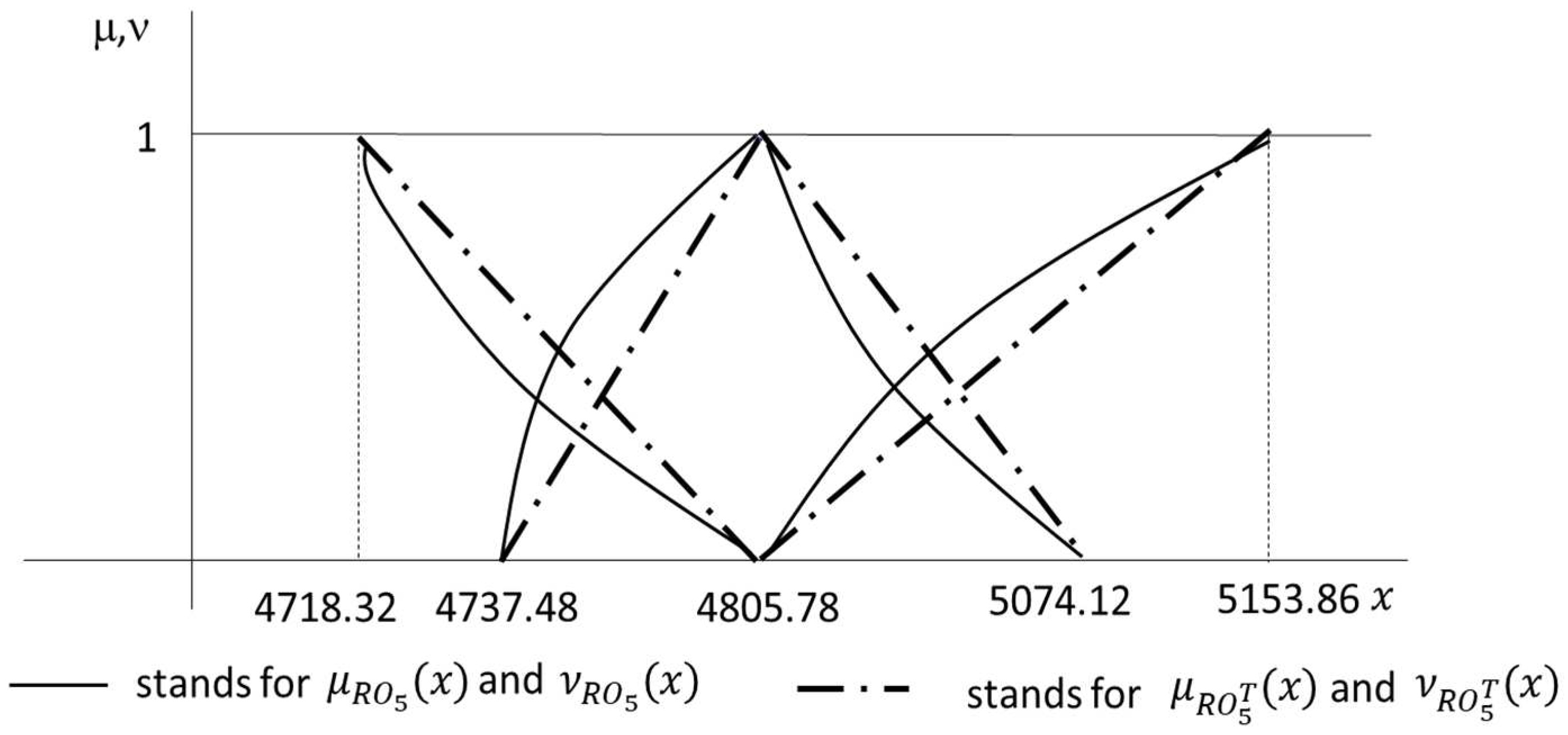
0	1	0.00%	0.00%	0.00%	0.00%	0.00%	0.00%	0.00%	0.00%

shows the $〈\alpha ,\beta 〉$-cuts of the estimates for the reserves associated with the fifth year of origin ${\widetilde{RO}}_5$ and the sixth calendar year ${\widetilde{RC}}_6$.

Table 12. $〈\alpha ,\beta 〉$-cuts of the overall claim intuitionistic fuzzy reserve and its triangular approximation.

α	$\beta$	${\underset{\_}{R}}_{\alpha }$	${\overline{R}}_{\alpha }$	${\underset{\_}{R^{*}}}_{\beta }$	${\overline{R^{*}}}_{\beta }$
1	0	9886.15	9886.15	9886.15	9886.15
0.75	0.25	9825.16	10,021.80	9807.79	10,061.07
0.5	0.5	9764.85	10,159.31	9730.54	10,239.09
0.25	0.75	9705.22	10,298.71	9654.40	10,420.25
0	1	9646.24	10,440.02	9579.34	10,604.62
${\tilde{R}}^{\prime }=(9886.15,239.91,306.81,553.87,718.48)$
α	$\beta$	${\underset{\_}{R^T}}_{\alpha }$	${\overline{R^T}}_{\alpha }$	${\underset{\_}{R^{T\mathrm{*}}}}_{\beta }$	${\overline{R^{T\mathrm{*}}}}_{\beta }$
1	0	9886.15	9886.15	9886.15	9886.15
0.75	0.25	9826.17	10,024.62	9809.45	10,065.77
0.5	0.5	9766.19	10,163.09	9732.75	10,245.39
0.25	0.75	9706.22	10,301.55	9656.04	10,425.01
0	1	9646.24	10,440.02	9579.34	10,604.62
α	$\beta$	${\underset{\_}{\epsilon }}_{\alpha }$	${\overline{\epsilon }}_{\alpha }$	${\underset{\_}{{\epsilon }^{\mathrm{*}}}}_{\beta }$	${\overline{{\epsilon }^{\mathrm{*}}}}_{\beta }$
1	0	0.00%	0.00%	0.00%	0.00%
0.75	0.25	0.01%	0.03%	0.02%	0.05%
0.5	0.5	0.01%	0.04%	0.02%	0.06
0.25	0.75	0.01%	0.03%	0.02%	0.05%
0	1	0.00%	0.00%	0.00%	0.00%

shows those for the total reserves $\tilde{R}$. In all the cases, we considered $〈\alpha ,1-\alpha 〉$, α = 0, 0.25, 0.5, 0.75, 1. The $〈\alpha ,\beta 〉$-cuts of their triangular approximations ${\widetilde{RO}}_5^T$, the calendar year ${\widetilde{RC}}_6^T$, and the total reserves $\widetilde{R^T}$ are also provided. We can observe that the linear approximation for all three reserves is practically perfect. The largest errors (5) are never greater than 0.06% and always in the $\beta$-cuts.

The set of $〈\alpha ,\beta 〉$-cuts of ${\widetilde{RO}}_5$, ${\widetilde{RC}}_6$ and $\tilde{R}$ in Table 11 and Table 12 can be interpreted as sensitivity assessments regarding the variability of reserves. The ability to include all reserves is maximal at $\alpha$= 0 and $\beta$= 1 (i.e., in the <0,1>-cut). However, the reserves estimated in this <0,1>-cut exhibit very low specificity. In contrast, in the <1,0>-cut, the specificity of the prediction is maximal, but it does not provide any estimation of possible deviations from the most plausible value. The interval between comprehensiveness and specificity may be the <0.5,0.5>-cut.

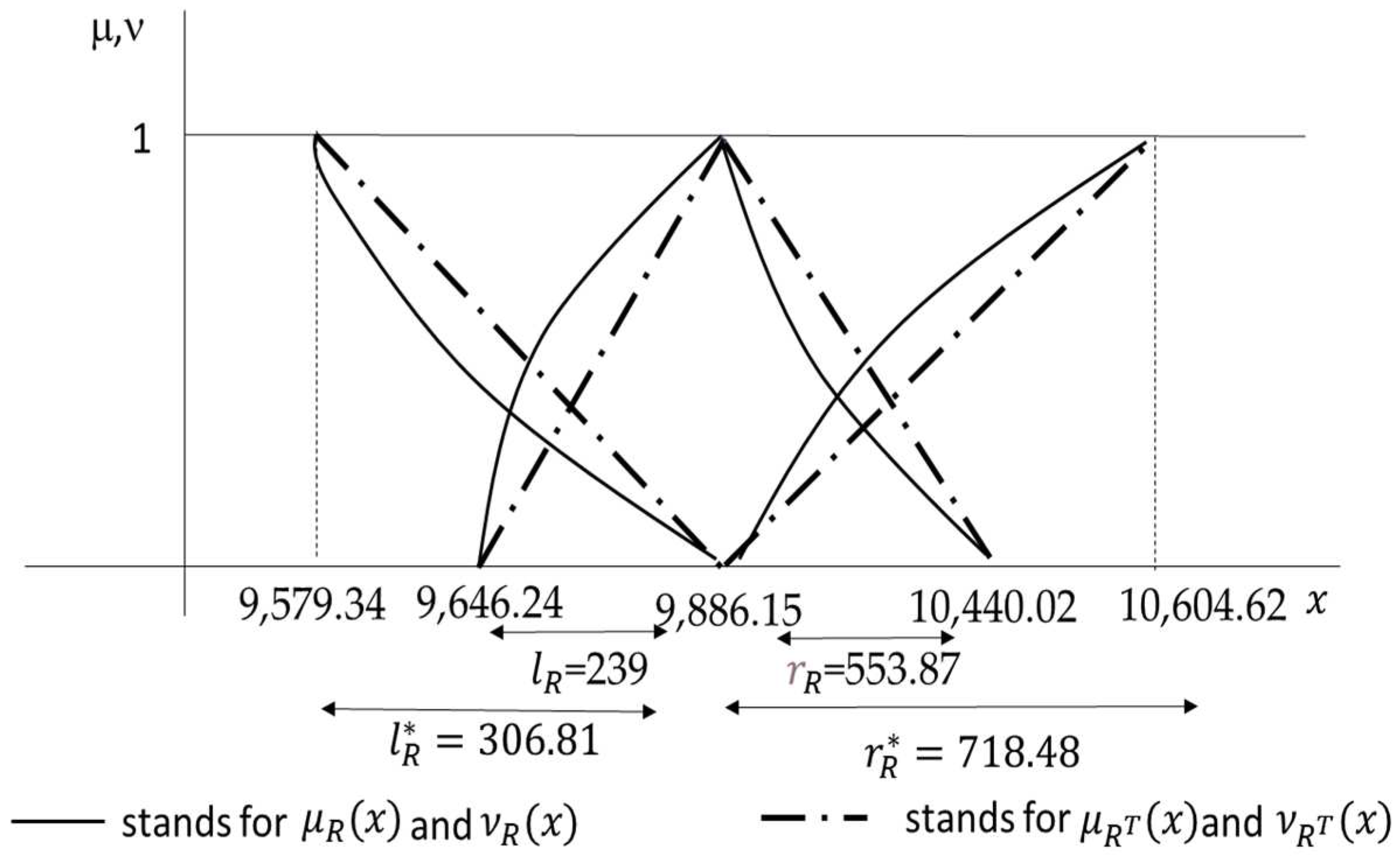
While Figure 4 and Figure 5 illustrate the shape of the intuitionistic fuzzy number that quantifies partial reserves and their triangular approximations, Figure 6 does so for the overall reserves. The information provided by the TIFN estimation of reserves is very intuitive for identifying an actuarial judgement and can also be interpreted as a structured sensitivity analysis of the adequate value for a set of five scenarios. The overall reserve with the highest reliability is 9886.15. The estimated deviations for these reserves are presented in the form of bipolar information, foreseeing possible maximum upper deviations of 553.87; in other words, the reserve to be allocated would be 10,443.02. Regardless, such fluctuations can never exceed 718.48, resulting in reserves of 10,604.62.

We can interpret the $〈\alpha ,\beta 〉$-cuts of reserves (Table 11 and Table 12) as similar to probabilistic intervals (Table 8). The equivalence between the α-cuts of possibility distributions and probabilistic confidence intervals has been extensively documented in the literature on probability–possibility transformations [64,65,66,67]. In this regard, it should be emphasized that the $\beta$-cut of the nonmembership function of an IFN can be interpreted as the (1 − $\beta$) of the upper possibility function [32]. Thus, the 0-cut of the membership function could be likened to probabilistic confidence intervals that include a majority of possible outcomes but not the most extreme ones. We refer, for example, to significance levels of 10% or 5%. Similarly, the 1-cut of the nonmembership function can be interpreted as a probabilistic confidence interval whose goal is to include practically all outcomes, which could be positioned at 0.5% or lower.

On the other hand, as shown in

Table 13. Evaluation of bootstrapping estimates of provisions on the intuitionistic estimat $\widetilde{R^T}=(9886.15,239.91,306.81,553.87,718.48)$.

Intuitionistic Fuzzy Evaluation of Reserves from a Bootstrapping Chain Ladder
Final value of reserves		${\mu }_{R^T}\left(x\right)$	${\nu }_{R^T}\left(x\right)$	$h_{R^T}\left(x\right)$
Point estimate	9899.31	0.976	0.018	0.005
50% percentile	9895.46	0.983	0.013	0.004
95% percentile	10,240.75	0.360	0.494	0.147
97.5% percentile	10,307.24	0.240	0.586	0.174
99.95% percentile	10,464.10	0.000	0.804	0.196
Intuitionistic fuzzy evaluation of reserves from bootstrapping two-way ANOVA
Final value of reserves		${\mu }_{R^T}\left(x\right)$	${\nu }_{R^T}\left(x\right)$	$h_{R^T}\left(x\right)$
Point estimate	9886.15	1.000	0.000	0.000
50% percentile	9888.24	0.996	0.003	0.001
95% percentile	10,014.75	0.768	0.179	0.053
97.5% percentile	10,042.19	0.718	0.217	0.065
99.95% percentile	10,150.23	0.523	0.368	0.109

, we can observe that the adjusted IFN reports the expressed level of reliability, from an intuitional point of view, regarding possible realizations of reserves. The tested values come from the point estimation and bootstrap estimates that accumulate 50%, 95%, 97.5%, and 99.95% probability. As we could expect, the point predictions and those associated with the 50th percentile have an almost total or total level of membership and an almost negligible level of nonmembership, with a degree of hesitancy that is almost nonexistent. The levels of membership, nonmembership, and hesitancy provide complementary measures to the accumulated probability levels that can be very useful for the decision maker in determining the final level of reserves, which should be prudent but not extremely unrealistic, thus unnecessarily burdening the insurer’s financial statements.

6. Discussion

A robust quantification of provisions for pending claims requires establishing a value with maximum reliability but also allowing for a margin of variability. While deterministic methods provide reliable values, stochastic methods can additionally estimate variability margins [2]. A third stream of methods, encompassing this work, involves modelling claims provisions through fuzzy quantities [10], which also entails predicting a reliable value and the variability of reserves.

The evolution of claims over time can be deterministically modelled, for example, with methods such as the chain ladder. However, the final determination of loss values is subject to deviations from deterministic predictions. Stochastic methods model these deviations by generalizing deterministic models through the random modelling of deviations [2]. Similarly, possibilistic models generalize these schemes under the assumption that the parameters governing claiming processes are fuzzy numbers (FNs). These include schemes such as the chain ladder [12,29], London chain ladder [11,27], Bornhuetter–Ferguson scheme [24], Taylor’s geometric separation method [14], and two-way models [16,17,18,19].

All the reviewed studies on loss reserving methods model uncertainty using type-1 fuzzy numbers, which are typically triangular and often symmetric. Our work extends these results by modelling parameters that govern claim processes with intuitionistic fuzzy numbers (IFNs). Notably, to the best of our knowledge, the application of intuitionistic logic to finance and actuarial issues is novel. In this regard, we can highlight applications in capital budgeting [33,34,35,36,38,39] and risk assessment [40].

The use of FNs in the context of actuarial and financial pricing allows for the introduction of epistemic uncertainty, that is, the perceived reliability of the possible values of the parameters of interest [10]. Therefore, FNs only allow the introduction of positive information about the feasible values of the parameter. On the other hand, intuitionistic fuzzy numbers (IFNs) permit bipolarity to be added by introducing both positive and negative information regarding variables of interest. In other words, it involves not only using estimated reliable values of the variables but also using unfeasible values [10].

The introduction of IFNs in determining loss reserves is carried out by generalizing the two-way ANOVA schema [42,43] and its possible extension [16], employing intuitionistic regression. The results of the comparison of the intuitionistic fuzzy method with two deterministic methods and their stochastic extensions suggest that it is able to produce useful results. Moreover, intuitionistic fuzzy quantifications can be interpreted as similar to the results obtained with stochastic methods. Furthermore, our method provides the possibility of assessing the membership and nonmembership of a possible final quantification in financial statements of loss provisions. Therefore, the results enrich the tools available to the actuary to exercise professional judgement, which is a fundamental step in the process of estimating claim reserves [3].

This study also contributes to the field of intuitionistic mathematics, specifically in a regression setting with a minimum fuzziness focus. While [41] generalizes possibilistic regression models [21,22], this work adapts the model from [23] to obtain IFN parameters. Thus, the estimates of the parameters governing the claiming process over time in our model are triangular IFNs (TIFNs) that are not necessarily symmetric. Our extension of intuitionistic regression can be applied in other financial and actuarial contexts where possibilistic regression has already been used, such as estimating the fuzzy temporal structure of interest rates [11], estimating mortality evolution [68], or estimating the implicit moments of options [69,70].

We focused on the use of input variables estimated by triangular IFNs and the approximation of the results obtained with linear shapes. Linear shapes often provide an effective resolution for practical applications of fuzzy set theory [46]. The interpretability of results by end users who may not necessarily have knowledge of fuzzy logic [46,58] is a desirable property of using TIFNs. The value of the reserves with TIFN parameters governing the two-way ANOVA system can be implemented with a very low error by evaluating five scenarios: one considered the maximum reliability scenario and two pairs of extreme positive and negative scenarios. Although the actuarial functions are nonlinear, they admit a good triangular approximation in accordance with the literature on fuzzy actuarial mathematics [11,12,14,58].

The extreme scenarios of intuitionistic fuzzy estimates can be interpreted within the concept of bipolar possibility [10]. The extreme scenarios associated with the values considered in the membership function can be understood as reasonable; those originating from the nonmembership measure potential extreme situations. Since the final determination of the provision value requires actuarial judgement, the intuitive interpretation of TIFNs favours their application.

The information that should be used in estimating pending claims is subject to various sources of vagueness, such as the scarcity of usable data, which tends to be current [9] and often imprecise [7]. The tools of fuzzy subset theory allow this kind of data to be handled. Therefore, generalizing our results to the case where observations of the run-off triangle are vague and modelled by fuzzy numbers or intuitionistic fuzzy numbers is feasible.

In recent years, other emerging techniques, such as neural networks (NNs) [71,72] and machine learning (ML) [73], have been applied to fit claim reserves in claim reserve calculations. Fuzzy and stochastic methods are implemented on the basis of classical schemes such as chain ladder. As an advantage of these novel approaches, [71,72,73] reported that they are capable of providing more accurate point estimates than classical methods. Therefore, they likely provide better estimates of the maximum likelihood value than the intuitionistic–fuzzy method proposed in this paper since the latter constructs the <1,0>-cut with the value of the classical method [42].

However, our method has two strengths compared to the methods of [71,72,73]. The first is that the adjusted parameters continue to have an economic interpretation, unlike those from deep learning techniques, where the adjusted parameters are more difficult to interpret. On the other hand, our intuitionistic fuzzy method fits bands of variability of reserves that incorporate bipolar information and are parameterized in a very natural way. In contrast, neural networks and machine learning techniques produce point estimates. In any case, deep learning methods and our intuitionistic fuzzy methods are not competitive but complementary. Whereas point estimates from NNs and ML techniques can be used as a reference for the maximum reliability values, intuitionistic fuzzy estimates provide a complete estimate of the uncertainty of these values.

7. Conclusions and Further Research

The uncertainty in the calculation of claim reserves has traditionally been caused by the introduction of stochastic variability into well-known calculation schemes such as the chain ladder or ANOVA two-way incremental claims. More recently, this uncertainty has been introduced by interpreting these schemes using possibilistic parameters in such a way that epistemic uncertainty is measured. This paper expands on the last stream of modelling uncertainty in calculations of claim reserves by introducing intuitionistic fuzzy parameters into the ANOVA two-way incremental claims schema. This methodology generalizes the possibilistic method [16], allowing the introduction of bipolar information about the value of parameters. This enhancement provides the actuary with more information to determine the final value of reserves than considering only epistemic uncertainty modelled stochastically or with fuzzy numbers.

A natural extension of this study involves introducing intuitionistic uncertainty in the analysis of nonlife insurance, as well as expanding the results obtained with fuzzy numbers to calculate discounted reserves [28], the discounted value of nonlife insurance liabilities [74], and the terminal value of an insurance company [75,76], using IFN parameters instead of FNs.

References

- Hindley, D. Introduction. In Claims Reserving in General Insurance; International Series on Actuarial Science; Cambridge University Press: Cambridge, UK, 2017; pp. 1–15. [Google Scholar]
- England, P.D.; Verrall, R.J. Stochastic claims reserving in general insurance. Br. Actuar. J. 2002, 8, 443–518. [Google Scholar] [CrossRef]
- Schmidt, K.D.; Zocher, M. The Bornhuetter-Ferguson. Variance 2008, 2, 85–110. Available online: https://www.casact.org/sites/default/files/2021-07/Bornhuetter-Ferguson-Schmidt-Zocher.pdf (accessed on 1 March 2024).
- Andrés Sánchez, J. Calculating insurance claim reserves with fuzzy regression. Fuzzy Sets Syst. 2006, 157, 3091–3108. [Google Scholar] [CrossRef]
- Lemaire, J. Fuzzy insurance. ASTIN Bull. J. IAA 1990, 20, 33–55. [Google Scholar] [CrossRef]
- Ostaszewski, K. An Investigation into Possible Applications of Fuzzy Sets Methods in Actuarial Science; Schaumburg (USA) Society of Actuaries: Schaumburg, IL, USA, 1993. [Google Scholar]
- Hindley, D. Data. In Claims Reserving in General Insurance; International Series on Actuarial Science; Cambridge University Press: Cambridge, UK, 2017; pp. 16–39. [Google Scholar]
- Shapiro, A.F. Fuzzy logic in insurance. Insur. Math. Econ. 2004, 35, 399–424. [Google Scholar] [CrossRef]
- Straub, E. Nonlife Insurance Mathematics; Springer: Berlin/Heidelberg, Germany, 1997. [Google Scholar]
- Dubois, D.; Prade, H. Gradualness, uncertainty and bipolarity: Making sense of fuzzy sets. Fuzzy Sets Syst. 2012, 192, 3–24. [Google Scholar] [CrossRef]
- Andrés-Sanchez, J.; Gómez, A.T. Applications of fuzzy regression in actuarial analysis. J. Risk Insur. 2003, 70, 665–699. [Google Scholar] [CrossRef]
- Heberle, J.; Thomas, A. Combining chain-ladder claims reserving with fuzzy numbers. Insur. Math. Econ. 2014, 55, 96–104. [Google Scholar] [CrossRef]
- Taylor, G. Separation of inflation and other effects from the distribution of non-life insurance claim delays. ASTIN Bull. 1977, 10, 217–230. [Google Scholar] [CrossRef]
- Apaydin, A.; Baser, F. Hybrid fuzzy least-squares regression analysis in claims reserving with geometric separation method. Insur. Math. Econ. 2010, 47, 113–122. [Google Scholar] [CrossRef]
- Yan, C.; Liu, Q.; Liu, J.; Liu, W.; Li, M.; Qi, M. Payments per claim model of outstanding claims reserve based on fuzzy linear regression. Int. J. Fuzzy Syst. 2019, 21, 1950–1960. [Google Scholar] [CrossRef]
- Andrés-Sánchez, J. Claim reserving with fuzzy regression and the two ways of ANOVA. Appl. Soft Comput. 2012, 12, 2435–2441. [Google Scholar] [CrossRef]
- Kim, J.H.; Kim, J. Fuzzy regression towards a general insurance application. J. Appl. Math. Inform. 2014, 32, 343–357. [Google Scholar] [CrossRef]
- Woundjiagué, A.; Bidima, M.L.D.M.; Mwangi, R.W. A fuzzy least-squares estimation of a hybrid log-Poisson regression and its goodness of fit for optimal loss reserves in insurance. Int. J. Fuzzy Syst. 2019, 21, 930–944. [Google Scholar]
- Woundjiagué, A.; Mbele Bidima, M.L.D.; Waweru Mwangi, R. An Estimation of a Hybrid Log-Poisson Regression Using a Quadratic Optimization Program for Optimal Loss Reserving in Insurance. Adv. Fuzzy Syst. 2019, 2019, 1393946. [Google Scholar] [CrossRef]
- Chukhrova, N.; Johannssen, A. Fuzzy regression analysis: Systematic review and bibliography. Appl. Soft Comput. 2019, 84, 105708. [Google Scholar] [CrossRef]
- Tanaka, H. Fuzzy data analysis by possibilistic linear models. Fuzzy Sets Syst. 1987, 24, 363–375. [Google Scholar] [CrossRef]
- Tanaka, H.; Ishibuchi, H. A possibilistic regression analysis based on linear programming. In Fuzzy Regression Analysis; Physica-Verlag: Heildelberg, Germany, 1992; pp. 47–60. [Google Scholar]
- Ishibuchi, H.; Nii, M. Fuzzy regression using asymmetric fuzzy coefficients and fuzzified neural networks. Fuzzy Sets Syst. 2001, 119, 273–290. [Google Scholar] [CrossRef]
- Heberle, J.; Thomas, A. The fuzzy Bornhuetter–Ferguson method: An approach with fuzzy numbers. Ann. Actuar. Sci. 2016, 10, 303–321. [Google Scholar] [CrossRef]
- Bastos, I.S.; Vana, L.B.; Novo, C.C. Estimating IBNR claim reserves using Gaussian Fuzzy Numbers. Context. Rev. Contemp. De Econ. E Gestão 2023, 21, 2. [Google Scholar] [CrossRef]
- Andrés-Sánchez, J. Claim reserving with fuzzy regression and Taylor’s geometric separation method. Insur. Math. Econ. 2007, 40, 145–163. [Google Scholar] [CrossRef]
- Baser, F.; Apaydin, A. Calculating insurance claim reserves with hybrid fuzzy least squares regression analysis. Gazi Univ. J. Sci. 2010, 23, 163–170. [Google Scholar]
- Andrés-Sánchez, J. Fuzzy claim reserving in nonlife insurance. Comput. Sci. Inf. Syst. 2014, 11, 825–838. [Google Scholar]
- Yan, C.; Liu, T.; Dong, Q.; Liu, W. Payments Per Claim Method Based on Fuzzy Numbers. In Proceedings of the 14th International Conference on Natural Computation, Fuzzy Systems and Knowledge Discovery (ICNC-FSKD), Huangshan, China, 28–30 July 2018; pp. 643–648. [Google Scholar] [CrossRef]
- Atanassov, K.T. Intuitionistic fuzzy sets. Fuzzy Sets Syst. 1986, 20, 87–96. [Google Scholar] [CrossRef]
- Atanassov, K.T. More on intuitionistic fuzzy sets. Fuzzy Sets Syst. 1989, 33, 37–45. [Google Scholar] [CrossRef]
- Mitchell, H.B. Ranking-intuitionistic fuzzy numbers. Int. J. Uncertain. Fuzziness Knowl.-Based Syst. 2004, 12, 377–386. [Google Scholar] [CrossRef]
- Kumar, G.; Bajaj, R.K. Implementation of intuitionistic fuzzy approach in maximizing net present value. Int. J. Math. Comput. Sci. 2014, 8, 1069–1073. [Google Scholar]
- Kahraman, C.; Çevik Onar, S.; Öztayşi, B. Engineering economic analyses using intuitionistic and hesitant fuzzy sets. J. Intell. Fuzzy Syst. 2015, 29, 1151–1168. [Google Scholar] [CrossRef]
- Boltürk, E.; Kahraman, C. Interval-valued and circular intuitionistic fuzzy present worth analyses. Informatica 2022, 33, 693–711. [Google Scholar] [CrossRef]
- Haktanır, E.; Kahraman, C. Intuitionistic fuzzy risk adjusted discount rate and certainty equivalent methods for risky projects. Int. J. Prod. Econ. 2023, 257, 108757. [Google Scholar] [CrossRef]
- Wu, L.; Liu, J.F.; Wang, J.T.; Zhuang, Y.M. Pricing for a basket of LCDS under fuzzy environments. SpringerPlus 2016, 5, 1747. [Google Scholar] [CrossRef] [PubMed]
- Ersen, H.Y.; Tas, O.; Kahraman, C. Intuitionistic fuzzy real-options theory and its application to solar energy investment projects. Eng. Econ. 2018, 29, 140–150. [Google Scholar] [CrossRef]
- Ersen, H.Y.; Tas, O.; Ugurlu, U. Solar Energy Investment Valuation with Intuitionistic Fuzzy Trinomial Lattice Real Option Model. IEEE Trans. Eng. Manag. 2023, 70, 2584–2593. [Google Scholar] [CrossRef]
- Uzhga-Rebrov, O.; Grabusts, P. Methodology for Environmental Risk Analysis Based on Intuitionistic Fuzzy Values. Risks 2023, 11, 88. [Google Scholar] [CrossRef]
- Parvathi, R.; Malathi, C.; Akram, M.; Atanassov, K. Intuitionistic fuzzy linear regression analysis. Fuzzy Optim Decis Mak. 2013, 12, 215–229. [Google Scholar] [CrossRef]
- Kremer, E. IBNR-claims and the two-way model of ANOVA. Scand. Actuar. J. 1982, 1982, 47–55. [Google Scholar] [CrossRef]
- Christofides, S. Regression models based on log-incremental payments. In Institute of Actuaries; Claims Reserving Manual; Institute of Actuaries: London, UK, 1990; Volume 2. [Google Scholar]
- Zadeh, L.A. Fuzzy sets. Inf. Control 1965, 8, 338–353. [Google Scholar] [CrossRef]
- Dubois, D.; Prade, H. Fuzzy numbers: An overview. In Readings in Fuzzy Sets Intelligent Systems; Dubois, D., Prade, H., Yager, R.R., Eds.; Elsevier: Amsterdam, The Netherlands, 1993; pp. 112–148. [Google Scholar] [CrossRef]
- Kreinovich, V.; Kosheleva, O.; Shahbazova, S.N. Why Triangular and Trapezoid Membership Functions: A Simple Explanation. In Recent Developments in Fuzzy Logic and Fuzzy Sets; Studies in Fuzziness and Soft Computing; Shahbazova, S., Sugeno, M., Kacprzyk, J., Eds.; Springer: Cham, Switzerland, 2020; Volume 391. [Google Scholar] [CrossRef]
- Yuan, X.H.; Li, H.X.; Zhang, C. The theory of intuitionistic fuzzy sets based on the intuitionistic fuzzy special sets. Inf. Sci. 2014, 277, 284–298. [Google Scholar] [CrossRef]
- Kumar, P.S.; Hussain, R.J. A method for solving unbalanced intuitionistic fuzzy transportation problems. Notes Intuitionistic Fuzzy Sets 2015, 21, 54–65. [Google Scholar]
- Mahapatra, G.S.; Roy, T.K. Intuitionistic fuzzy number and its arithmetic operation with application on system failure. J. Uncertain Syst. 2013, 7, 92–107. [Google Scholar]
- Bhaumik, A.; Roy, S.K.; Li, D.F. Analysis of triangular intuitionistic fuzzy matrix games using robust ranking. J. Intell. Fuzzy Syst. 2017, 33, 327–336. [Google Scholar] [CrossRef]
- Rasheed, F.; Kousar, S.; Shabbir, J.; Kausar, N.; Pamucar, D.; Gaba, Y.U. Use of intuitionistic fuzzy numbers in survey sampling analysis with application in electronic data interchange. Complexity 2021, 2021, 9989477. [Google Scholar] [CrossRef]
- Bayeg, S.; Mert, R. On intuitionistic fuzzy version of Zadeh’s extension principle. Notes Intuitionistic Fuzzy Sets 2021, 27, 9–17. [Google Scholar] [CrossRef]
- Nguyen, H.T. A note on the extension principle for fuzzy sets. J. Math. Anal. Appl. 1978, 64, 369–380. [Google Scholar] [CrossRef]
- Dong, W.; Shah, H.C. Vertex method for computing functions of fuzzy variables. Fuzzy Sets Syst. 1987, 24, 65–78. [Google Scholar] [CrossRef]
- Buckley, J.J.; Qu, Y. On using α-cuts to evaluate fuzzy equations. Fuzzy Sets Syst. 1990, 38, 309–312. [Google Scholar] [CrossRef]
- Jiménez, M.; Rivas, J.A. Fuzzy number approximation. Int. J. Uncertain. Fuzziness Knowl.-Based Syst. 1998, 6, 69–78. [Google Scholar] [CrossRef]
- Villacorta, P.J.; González-Vila Puchades, L.; de Andrés-Sánchez, J. Fuzzy Markovian Bonus-Malus Systems in Nonlife Insurance. Mathematics 2021, 9, 347. [Google Scholar] [CrossRef]
- Andrés-Sánchez, J.; González-Vila Puchades, L. Life settlement pricing with fuzzy parameters. Appl. Soft Comput. 2023, 148, 110924. [Google Scholar] [CrossRef]
- Savic, D.; Predrycz, W. Fuzzy linear models: Construction and evaluation. In Fuzzy Regression Analysis; Physica-Verlag: Heildelberg, Germany, 1992; pp. 91–100. [Google Scholar]
- Chen, F.; Chen, Y.; Zhou, J.; Liu, Y. Optimizing h value for fuzzy linear regression with asymmetric triangular fuzzy coefficients. Eng. Appl. Artif. Intell. 2016, 47, 16–24. [Google Scholar] [CrossRef]
- Schmidt, K.D.; Zocher, M. Additive Method. In Handbook on Loss Reserving; EAA Series; Radtke, M., Schmidt, K.D., Schnaus, A., Eds.; Springer: Cham, Switzerland, 2016. [Google Scholar] [CrossRef]
- England, P.D.; Verrall, R. Analytic and bootstrap estimates of prediction errors in claims reserving. Insur. Math. Econ. 1999, 25, 281–293. [Google Scholar] [CrossRef]
- The Faculty and Institute of Actuaries. Claims Reserving Manual, 2nd ed.; The Faculty and Institute of Actuaries: London, UK, 1997; Volume 1. [Google Scholar]
- Couso, I.; Montes, S.; Gil, P. The necessity of the strong α-cuts of a fuzzy set. Int. J. Uncertain. Fuzziness Knowl.-Based Syst. 2001, 9, 249–262. [Google Scholar] [CrossRef]
- Dubois, D.; Folloy, L.; Mauris, G.; Prade, H. Probability–possibility transformations, triangular fuzzy sets, and probabilistic inequalities. Reliab. Comput. 2004, 10, 273–297. [Google Scholar] [CrossRef]
- Sfiris, D.S.; Papadopoulos, B.K. Nonasymptotic fuzzy estimators based on confidence intervals. Inf. Sci. 2014, 279, 446–459. [Google Scholar] [CrossRef]
- Adjenughwure, K.; Papadopoulos, B. Fuzzy-statistical prediction intervals from crisp regression models. Evol. Syst. 2020, 11, 201–213. [Google Scholar] [CrossRef]
- Andrés Sánchez, J.; Gonzalez-Vila, L. A fuzzy-random extension of the Lee-Carter mortality prediction model. Int. J. Comput. Intell. Syst. 2019, 12, 775–794. [Google Scholar] [CrossRef]
- Muzzioli, S.; Gambarelli, L.; De Baets, B. Option implied moments obtained through fuzzy regression. Fuzzy Optim. Decis. Mak. 2020, 19, 211–238. [Google Scholar] [CrossRef]
- Muzzioli, S.; Ruggieri, A.; De Baets, B. A comparison of fuzzy regression methods for the estimation of the implied volatility smile function. Fuzzy Sets Syst. 2015, 266, 131–143. [Google Scholar] [CrossRef]
- Kuo, K. Deep triangle: A deep learning approach to loss reserving. Risks 2019, 7, 97. [Google Scholar] [CrossRef]
- Wüthrich, M.V. Neural networks applied to chain–ladder reserving. Eur. Actuar. J. 2018, 8, 407–436. [Google Scholar] [CrossRef]
- Wüthrich, M.V. Machine learning in individual claims reserving. Scand. Actuar. J. 2018, 2018, 465–480. [Google Scholar] [CrossRef]
- Cummins, D.J.; Derrig, R.A. Fuzzy financial pricing of property-liability insurance. N. Am. Actuar. J. 1997, 1, 21–40. [Google Scholar] [CrossRef]
- Mircea, I.; Covrig, M. A discrete time insurance model with reinvested surplus and a fuzzy number interest rate. Procedia Econ. Financ. 2015, 32, 1005–1011. [Google Scholar] [CrossRef]
- Ungureanu, D.; Vernic, R. On a fuzzy cash flow model with insurance applications. Decis. Econ. Financ. 2015, 38, 39–54. [Google Scholar] [CrossRef]
Figure 1.
Triangular intuitionistic fuzzy numbers.
Figure 2.
Intuitionistic fuzzy number estimation of the logarithm of the incremental claim baseline (.
Figure 3.
Intuitionistic fuzzy number estimate of the growth rate of claims for the origin year i = 1 ( and for the development year j = 1 (.
Figure 4.
Intuitionistic fuzzy number estimation of the reserves of development year i = 5 ( and its triangular approximate .
Figure 5.
Intuitionistic fuzzy number estimation of the reserves of calendar year i + j = 6 ( and its triangular approximation .
Figure 6.
Intuitionistic fuzzy number estimation of overall reserves ( and its triangular approximation ().