Improving Realism of Facial Interpolation and Blendshapes with Analytical Partial Differential Equation-Represented Physics

Abstract

How to create realistic shapes by interpolating two known shapes for facial blendshapes has not been investigated in the existing literature. In this paper, we propose a physics-based mathematical model and its analytical solutions to obtain more realistic facial shape changes. To this end, we first introduce the internal force of elastic beam bending into the equation of motion and integrate it with the constraints of two known shapes to develop the physics-based mathematical model represented with dynamic partial differential equations (PDEs). Second, we propose a unified mathematical expression of the external force represented with linear and various nonlinear time-dependent Fourier series, introduce it into the mathematical model to create linear and various nonlinear dynamic deformations of the curves defining a human face model, and derive analytical solutions of the mathematical model. Third, we evaluate the realism of the obtained analytical solutions in interpolating two known shapes to create new shape changes by comparing the shape changes calculated with the obtained analytical solutions and geometric linear interpolation to the ground-truth shape changes and conclude that among linear and various nonlinear PDE-based analytical solutions named as linear, quadratic, and cubic PDE-based interpolation, quadratic PDE-based interpolation creates the most realistic shape changes, which are more realistic than those obtained with the geometric linear interpolation. Finally, we use the quadratic PDE-based interpolation to develop a facial blendshape method and demonstrate that the proposed approach is more efficient than numerical physics-based facial blendshapes.

1. Introduction

Facial interpolation and blendshapes are the most popular tools in quickly creating many different facial expressions from known facial expressions. Realistic facial expressions play a crucial role in conveying the motions, personality, and intentions of a human character and communicating with others. It is the most important part of character animation. Despite the popularity of facial interpolation and blendshapes, we have not found any research studies which investigate how to use shape interpolation to create more realistic facial expressions from two known facial expressions.

Shape interpolation is to create new shapes from known shapes. It is widely applied in facial blendshapes. Various shape interpolation methods have been developed. Among them, geometric linear interpolation, which is the case of a linear model with two known shapes, is widely used to create new facial shapes between two known shapes.

As discussed in [1], facial movements and deformations are highly nonlinear since a human face is a very complicated biomechanical system consisting of skeletons, muscles, flesh, skin, and other tissues. One such example is human jaw movement. The real orbit of a vertex on the chin is roughly an arc centred at the temporomandibular joint, as shown by the light blue curve in Figure 1a. When the geometric linear interpolation is used to create new shapes of human jaw movement between ω = 0 and ω = 1, the orbit of the vertex on the chin is a straight line, as shown by the purple line in Figure 1b. Another such example is the closing movement of human eyes. The trail of real eyelid movements should follow the contour of the corner shown by the light blue curve in Figure 2a. When the geometric linear interpolation is used to create new shapes between ω = 0 and ω = 1, the trail is a straight line highlighted in purple in Figure 2b.

Apart from the geometric linear interpolation, other geometric interpolation methods have also been proposed. These methods include cosine interpolation, etc. Besides the linear model, bilinear, multilinear, and nonlinear models are also proposed. Despite this, no research studies investigate how to choose a proper interpolation method to create more realistic shape changes from two known shapes. The work carried out in [1] investigates how to achieve more realistic facial blendshapes with a cubic polynomial and about 500 known facial expressions by solving an optimisation problem involving over 30,000 optimisation variables. It is not applicable to the case investigated in this paper, where only two facial expressions are known.

Since geometric linear and nonlinear interpolation methods do not consider the underlying physics of facial movements, physics-based facial blendshapes have been developed. However, physics-based facial blendshapes usually involve heavy numerical calculations and are not suitable for facial animation requiring high computational efficiency.

To tackle the problems of poor realism of geometric interpolation and low efficiency of physics-based facial blendshapes, this paper will propose a new, efficient, and realistic shape interpolation method. We first propose a PDE-represented physics model and derive its analytical solutions. Then, we introduce two known facial expressions to determine unknown constants in the analytical solutions. After that, we evaluate and identify the most suitable analytical solution. Finally, we use the most suitable analytical solution to create more realistic facial shapes.

2. Related Work

The work proposed in this paper will introduce PDE-represented physics to develop a more realistic and efficient method of facial interpolation and facial blendshapes. In this section, we briefly review existing work in facial blendshapes and PDE-based geometric modelling.

2.1. Facial Blendshapes

Many methods for facial blendshapes have been developed. Among them, geometric and physics-based facial blendshapes are very popular.

Geometric facial blendshapes create new facial shapes from known ones. Linear, bilinear, and multilinear models have been proposed to generate facial blendshapes. Among them, the linear model is most widely applied in computer animation.

The linear model presents a linear weighted combination of known facial shapes. A comprehensive review of facial blendshapes based on the linear model is made in [2]. When only two facial shapes are known, the linear model becomes the geometric linear interpolation [3], which has been combined with the facial action coding system (FACS) to create a computer facial animation design [4]. Apart from the geometric linear interpolation, nonlinear interpolation, such as a cosine interpolation function [5], is also proposed to provide some special effects.

The linear model has been used to develop various facial blendshape methods. A direct manipulation method is presented in [6], which integrates linear model-based facial blendshapes and user interaction to manipulate facial meshes. A framework is proposed in [7] to automatically create optimal facial blendshapes from example poses of a facial model. Facial mesh vertices are modified in [8] through iterative optimisation from captured facial movements. The linear model is used to capture facial details through automatically generating localised blendshapes and incrementally adding a blendshape to obtain missing source features [9]. It has also been used to develop an approach of splitting a face mesh into natural clusters and connecting each mesh segment with the relevant set of deformation controllers [10]. By using Laplacian smoothing to separate a three-dimensional model into a smoothed mesh and separated details, the linear model is used to obtain a linear combination of the separated details from multiple three-dimensional models and add the linear combination to the smoothed mesh of a target model to achieve facial blendshapes [11].

Besides the linear model, bilinear, multilinear, and nonlinear models have also been developed. Bilinear models are used in [12] to separate style and content. They are introduced in [13] to recognise three-dimensional faces and facial expressions. The multilinear model is used to parameterise the space of geometric variations caused by identity, expression, and viseme [14]. The nonlinear model is proposed to develop an interactive facial animation editing system [15], which first computes blendshape weights from the linearly constrained quadratic optimisation and then nonlinearly interpolates the deformation gradients of blendshapes to update the blendshape weights and facial mesh vertices.

Although various geometric facial blendshape methods have been developed, we are unaware of any work that investigates how to interpolate two known shapes to create realistic shapes. This problem will be tackled in this paper.

Physics-based facial blendshapes introduce the underlying physics to create more realistic facial shape changes. Ma et al. integrate physical-based simulation into blendshapes by constructing a mass-spring system for each blendshape target, linearly interpolating the rest lengths of the springs, and calculating the equilibrium of the mass-spring system to achieve physics-based blendshapes [16]. Hahn et al. unify keyframing and physical simulation by using tetrahedral finite elements to solve Newton’s second law for standard Saint-Venant Kirchhoff or Neo-Hookean material models [17]. Instead of using a basis of shapes, Barrielle et al. use a basis of forces for blendshapes to encode facial dynamics that simulate mesh deformations by integrating the blendshape paradigm and physics-based techniques through finite element modelling of the face as an elastic thin shell [18]. Different from the methods of adding physics to face rigs, Kozlov et al. propose to add physics to facial blendshape animation by using a blendvolume rig that enriches blendshape rigs with a simple volumetric tissue structure and shape-dependent material parameters called blendmaterials through finite element-based simulation [19]. Ichim et al. use tetrahedral meshes to discretise the soft tissue of the face, formulate a set of nonlinear potential energies to simulate the physical interaction of passive flesh, active muscles, and rigid bone structures with linear finite elements and minimise the nonlinear potential energies to achieve physics-based facial animation [20]. Wagner et al. present a neural network and physics-based approach to achieve physics-based facial blendshapes [21].

Since physics-based facial blendshapes consider the underlying physics, they create more realistic facial shape changes. However, they involve heavy numerical calculations such as mass-spring and finite element simulations. This issue will be addressed by developing analytical and efficient physics-based facial blendshapes.

2.2. PDE-Based Geometric Modelling

The research into PDE-based geometric modelling was pioneered by Bloor and Wilson [22]. After that, many research studies have been carried out to develop various PDE-based geometric modelling methods.

Ugail et al. develop efficient techniques that construct PDE surfaces interactively in real-time [23]. Monterde and Ugail introduce a general fourth-order partial differential equation to generate Bézier surfaces from boundary information [24]. Xu and Zhang use geometric partial differential equations to develop a general framework for surface modelling [25]. You et al. present a dynamic skin deformation method based on a time-dependent partial differential equation [26]. Castro et al. make a comprehensive survey on partial differential equation-based geometric design [27]. Sheng et al. propose a patchwise partial differential equation function representation and use it to replace large polygon meshes [28]. Ugail gives a detailed description of geometric design using partial differential equations [29]. Sheng et al. use spectral solutions to fourth-order elliptic PDEs to produce and animate three-dimensional facial geometry [30]. Pan et al. combine geometric partial differential equations with surface subdivision to develop a unified method for freeform surface design [31]. Chen et al. visualise computed tomography data of human heads through partial differential equation-based surface reconstruction [32]. Wang et al. investigate how to optimally convert PDE surface-represented high-speed train heads into NURBS surfaces [33]. You et al. introduce partial differential equations to develop a physics-based deformation method for creating detailed three-dimensional virtual character models [34]. Wang et al. integrate partial differential equation-based geometric modelling and boundary-based surface creation to obtain the first analytical $C^0$ continuous four-sided PDE patches [35]. Zhu et al. use a fourth-order partial differential equation to reconstruct three-dimensional surfaces from multi-view two-dimensional images [36]. Fu et al. propose a time-independent static second-order partial differential equation of two parametric variables $u$ and $v$ without involving any forces, derived its analytical solution, and used the analytical solution and geometric linear interpolation to generate new models from a neutral shape and a target shape or from a neutral shape and more than one target shape [37]. Since the static PDE has no ability to describe shape changes, geometric linear interpolation is used to interpolate PDE surfaces for creating new facial models from existing facial models. Due to this reason, the method proposed in [37] is unable to achieve more realistic facial interpolation than the geometric linear interpolation, as discussed in Section 4.3 of this paper.

Although there are extensive research studies about PDE-based geometric modelling, we have not found any work that investigates how to use PDE-based geometric modelling to achieve more realistic facial interpolation from two known facial shapes. In this paper, we will propose a time-dependent dynamic partial differential equation involving a parametric variable $u$, a time variable $t$, an inertia force, a damping force, an internal deformation force, and an external force to describe facial shape changes with underlying physics and develop a physics-based analytical method to achieve more realistic facial shape interpolation and facial blendshapes than the geometric linear interpolation.

3. PDE-Represented Physics and Analytical Solution

In existing work, the equation of motion has been widely applied in computer graphics to simulate physics-based facial animation [38,39,40,41,42] and muscle and skin deformations [41]. It has the following form:

$$\begin{gathered} m\frac{{\partial }^{2}w}{\partial t^2}+c\frac{\partial w}{\partial t}+q_w=f_w \\ (w=x, y, z) \end{gathered}$$

(1)

where $w$ is a position function, which has three components $x$, $y$, and $z$, $m$ and $c$ denote mass and damping coefficient, respectively, $q_w$ is an internal deformation force and $f_w$ is an external force.

The surface model of a human face can be defined with a set of curves. The deformation of each of the curves can be described by the following equation, which is similar to the governing equation describing the elastic bending of a beam.

$${k\frac{{\partial }^{4}w}{\partial u^4}=\overline{q}}_w$$

(2)

where the flexural rigidity $k=EI$, $E$ is the modulus of elasticity, $I$ is the moment of inertia, $k\frac{{\partial }^{4}w}{\partial u^4}$ is the internal deformation force and ${\overline{q}}_w$ is the external force.

Using the internal deformation force $k\frac{{\partial }^{4}w}{\partial u^4}$ to replace $q_w$ in Equation (1), the equation of motion becomes the following time-dependent dynamic partial differential Equation:

$$m\frac{{\partial }^{2}w}{\partial t^2}+c\frac{\partial w}{\partial t}+k\frac{{\partial }^{4}w}{\partial u^4}=f_w$$

(3)

In the above Equation, the first term is the inertia force caused by acceleration, the second term is the damping force caused by velocity, and the third term is the internal deformation force caused by curve deformation. The position function $w$ and the external force $f_w$ are the functions of the time variable $t$ and the parametric variable $u$, i.e., $w=w(u,t)$ and $f_w=f_w(u,t)$.

Shape interpolation is to generate new shapes from two known shapes, i.e., a neutral shape and a target shape. If we use $w_0\left(u\right)$ and $w_1\left(u\right)$ to indicate the known neutral shape at $t=0$ and the known target shape at $t=1$, respectively, the boundary conditions for Equation (3) can be written as follows:

$$\begin{gathered} t=0 w\left(u,t\right)=w_0\left(u\right) \\ t=1 w\left(u,t\right)=w_1\left(u\right) \end{gathered}$$

(4)

Equations (3) and (4) are the mathematical model of physics-based facial interpolation and facial blendshapes. The task of physics-based shape interpolation is to solve the mathematical model.

Numerical methods such as the finite difference method are very effective in solving the mathematical model represented by Equations (3) and (4). However, these numerical methods involve heavy calculations, require large computer resources, and do not suit situations such as computer animation where high computational efficiency is required. To address the disadvantages of numerical methods, we derive an analytical solution $w\left(u,t\right)$ to Equation (3) subjected to boundary conditions (4) in this section.

At a time instant $t$, $w\left(u,t\right)=w\left(u\right)$ indicates a spatial curve, which can be described with a Fourier series. According to Equation (4), two position boundary conditions are known, which can be used to determine two unknown constants in the analytical solution $w\left(u,t\right)$. It means the external force $f_w(u,t)$ should involve two unknown coefficients to be determined with the two position boundary conditions. To tackle both linear and various nonlinear shape changes, the external force should be represented with linear and various nonlinear functions of the time variable $t$. Based on these considerations, the external force is taken to be a combination of a $R^{th}$ order polynomial of the time variable $t$ with two unknown coefficients and a Fourier series of the parametric variable $u$, i.e.,

$$\begin{gathered} f_w(u,t)={\overline{e}}_{w0}+{\stackrel{̿}{e}}_{w0}{t}^R+{\sum }_{n=1}^N\left[\right({\widehat{e}}_{wn}+{\check{e}}_{wn}{t}^R)cos2n\pi u+({\tilde{e}}_{wn}+{\overline{e}}_{wn}{t}^R\left)sin2n\pi u\right] \\ (w=x, y, z; R=1, 2, 3,\dots ) \end{gathered}$$

(5)

where ${\overline{e}}_{w0}$, ${\stackrel{̿}{e}}_{w0}$, ${\widehat{e}}_{wn}$, ${\check{e}}_{wn}$, ${\tilde{e}}_{wn}$, and ${\overline{e}}_{wn}$ ($n=1, 2, 3, \dots , N$) are unknown coefficients, which are related to the position function through Equation (3), and $R$ indicates the order of the polynomial. $R=1$ and $R>1,$ respectively, describe a linear change and various nonlinear changes of the external force against the time variable $t$.

According to the external force (5) and Equation (3), the analytical solution to Equation (3) should have the following form:

$$w(u,t)=g_{w0}\left(t\right)+{\sum }_{n=1}^N\left[{\overline{g}}_{wn}\left(t\right)\right.cos2n\pi u+{\stackrel{̿}{g}}_{wn}(\mathrm{t})sin2n\pi u]$$

(6)

Substituting Equations (5) and (6) into (3), Equation (3) is changed into the following ordinary differential Equation:

$$\begin{gathered} m\frac{{d^{2}g}_{w0}\left(t\right)}{d{t}^2}+m\sum _{n=1}^N\left[\frac{d^2{\overline{g}}_{wn}\left(t\right)}{d{t}^2}\right.cos2n\pi u+\left.\frac{d^2{\stackrel{̿}{g}}_{wn}\left(t\right)}{d{t}^2}sin2n\pi u\right]+c\frac{{dg}_{w0}\left(t\right)}{dt} \\ +c\sum _{n=1}^N\left[\frac{d{\overline{g}}_{wn}\left(t\right)}{dt}\right.cos2n\pi u+\left.\frac{d{\stackrel{̿}{g}}_{wn}\left(t\right)}{dt}sin2n\pi u\right] \\ +16k{\pi }^4\sum _{n=1}^N{n}^4\left[{\overline{g}}_{wn}\left(t\right)\right.cos2n\pi u+{\stackrel{̿}{g}}_{wn}(\mathrm{t})sin2n\pi u]={\overline{e}}_{w0}+{\stackrel{̿}{e}}_{w0}{t}^R \\ +{\sum }_{n=1}^N\left[\right({\widehat{e}}_{wn}+{\check{e}}_{wn}{t}^R)cos2n\pi u+({\tilde{e}}_{wn}+{\overline{e}}_{wn}{t}^R\left)sin2n\pi u\right] \end{gathered}$$

(7)

The above ordinary differential Equation is equivalent to the following three ordinary differential Equations:

$$m\frac{{d^{2}g}_{w0}\left(t\right)}{d{t}^2}+c\frac{{dg}_{w0}\left(t\right)}{dt}={\overline{e}}_{w0}+{\stackrel{̿}{e}}_{w0}{t}^R$$

(8)

$$m\frac{d^2{\overline{g}}_{wn}\left(t\right)}{d{t}^2}+c\frac{d{\overline{g}}_{wn}\left(t\right)}{dt}+16k{n}^4{\pi }^4{\overline{g}}_{wn}\left(t\right)={\widehat{e}}_{wn}+{\check{e}}_{wn}{t}^R$$

(9)

$$m\frac{d^2{\stackrel{̿}{g}}_{wn}\left(t\right)}{d{t}^2}+c\frac{d{\stackrel{̿}{g}}_{wn}\left(t\right)}{dt}+16k{n}^4{\pi }^4{\stackrel{̿}{g}}_{wn}(t)={\tilde{e}}_{wn}+{\overline{e}}_{wn}{t}^R$$

(10)

In what follows, we investigate how to obtain the analytical solutions to each of the above three ordinary differential equations.

3.1. Analytical Solution of Equation (8)

Since the right-hand side term of Equation (8) is a polynomial, we can use the method of undetermined coefficients to solve it. The analytical solution is taken to be as follows:

$$g_{w0}\left(t\right)={\sum }_{r=0}^{R+1}{b}_{wr}{t}^r$$

(11)

Substituting Equation (11) and its first and second derivatives with the time variable $t$ into the ordinary differential Equation (8), we obtain the following:

$$m{\sum }_{r=2}^{R+1}{r\left(r-1\right)b}_{wr}{t}^{r-2}+c{\sum }_{r=1}^{R+1}{rb}_{wr}{t}^{r-1}={\overline{e}}_{w0}+{\stackrel{̿}{e}}_{w0}{t}^R$$

(12)

The above Equation can be further changed into the following form:

$$m{\sum }_{r=0}^{R-1}{(r+1)(r+2)b}_{wr+2}{t}^r+c{\sum }_{r=0}^{R-1}(r+1)b_{wr+1}{t}^r+c{(R+1)b}_{wR+1}{t}^R={\overline{e}}_{w0}+{\stackrel{̿}{e}}_{w0}{t}^R$$

(13)

Equaling the terms of $t^R$ in the above Equation, the unknown constant $b_{wR+1}$ is obtained as follows:

$$b_{wR+1}=\frac{{\stackrel{̿}{e}}_{w0}}{c(R+1)}$$

(14a)

Equaling the terms of $t^r$ ($r=R-1, R-2, R-3, \dots , 3, 2, 1$), the unknown constant $b_{wr+1}$ are obtained as follows:

$$\begin{gathered} b_{wr+1}=-\frac{m\left(r+2\right)b_{wr+2}}{c} \\ (r=R-1, R-2, R-3, \dots , 3, 2, 1) \end{gathered}$$

(14b)

Equaling the terms of $t^0$, the unknown constant $b_{w1}$ are obtained as follows:

$$b_{w1}=({\overline{e}}_{w0}-2m{b}_{w2})/c$$

(14c)

In this paper, we investigate how linearly ($R=1$), quadratically ($R=2$), and cubically ($R=2$) varying external forces affect the realism of shape interpolation.

For a linearly varying external force, $R=1$. The unknown constants are obtained from Equations (14a) and (14c).

$$\begin{gathered} b_{w1}=\frac{{\overline{e}}_{w0}}{c}-m{\stackrel{̿}{e}}_{w0}/c^2 \\ {b}_{w2}={\stackrel{̿}{e}}_{w0}/\left(2c\right) \end{gathered}$$

(15)

For a quadratically varying external force, $R=2$. The unknown constants are obtained from Equations (14a)–(14c)

$$\begin{gathered} b_{w1}=\frac{{\overline{e}}_{w0}}{c}+{2m}^2{\stackrel{̿}{e}}_{w0}/c^3 \\ {b}_{w2}=-\frac{m{\stackrel{̿}{e}}_{w0}}{c^2} \\ {b}_{w3}={\stackrel{̿}{e}}_{w0}/\left(3c\right) \end{gathered}$$

(16)

For a cubically varying external force, $R=3$. Same as above, the unknown constants are obtained from Equations (14a)–(14c)

$$\begin{gathered} b_{w1}=\frac{{\overline{e}}_{w0}}{c}-\frac{{6m}^3{\stackrel{̿}{e}}_{w0}}{c^4} \\ {b}_{w2}=\frac{{3m}^2{\stackrel{̿}{e}}_{w0}}{c^3} \\ {b}_{w3}=-\frac{m{\stackrel{̿}{e}}_{w0}}{c^2} \\ {b}_{w4}={\stackrel{̿}{e}}_{w0}/\left(4c\right) \end{gathered}$$

(17)

3.2. Analytical Solution of Equation (9)

With the same treatment, we take the analytical solution of Equation (9) to be as follows:

$${\overline{g}}_{wn}\left(t\right)={\sum }_{r=0}^R{c}_{wr}{t}^r$$

(18)

Substituting Equation (18) and its first and second derivatives with respect to the time variable $t$ into the ordinary differential Equation (9) and letting

$$B_n=16k{n}^4{\pi }^4$$

(19)

we obtain the following:

$$\begin{gathered} m{\sum }_{r=2}^{R}r\left(r-1\right)c_{wr}{t}^{r-2}+c{\sum }_{r=1}^{R}r{c}_{wr}{t}^{r-1}+B_n{\sum }_{r=0}^R{c}_{wr}{t}^r \\ ={\widehat{e}}_{wn}+{\check{e}}_{wn}{t}^R \end{gathered}$$

(20)

The above Equation can be further changed into the following form:

$$\begin{gathered} m{\sum }_{r=0}^{R-2}{\left(r+2\right)\left(r+1\right)c}_{wr+2}{t}^r+c{\sum }_{r=0}^{R-2}\left(r+1\right)c_{wr+1}{t}^r+c{Rc}_{wR}{t}^{R-1} \\ +B_n{c}_{wR-1}{t}^{R-1}+B_n{c}_{wR}{t}^R+B_n{\sum }_{r=0}^{R-2}{c}_{wr}{t}^r={\widehat{e}}_{wn}+{\check{e}}_{wn}{t}^R \end{gathered}$$

(21)

From the above Equation, the unknown constants can be obtained as follows:

$$\begin{gathered} c_{wR}={\check{e}}_{wn}/B_n \\ {c}_{wR-1}=-\frac{cR{c}_{wR}}{B_n}=-\frac{\frac{cR}{B_n}{\check{e}}_{wn}}{B_n}=-\frac{cR}{B_n^2}{\check{e}}_{wn} \mathrm{for} (R\ge 2) \\ {c}_{wr}=-[\left(r+2\right)\left(r+1\right)m{c}_{wr+2}+\left(r+1\right)c{c}_{wr+1}]/B_n \\ \hspace{1em} (r=R-2,R-3, R-4, \dots , 3, 2, 1) \\ {c}_{w0}={(\widehat{e}}_{wn}-2m{c}_{w2}-c{c}_{w1})/B_n \mathrm{for} (R\ge 2) \\ {c}_{w0}={(\widehat{e}}_{wn}-c{c}_{w1})/B_n \hspace{1em}\hspace{1em}\mathrm{for} (R=1) \end{gathered}$$

(22)

For a linearly varying external force, $R=1$. The unknown constants are obtained from Equation (22)

$$\begin{gathered} c_{w0}={(\widehat{e}}_{wn}-c{c}_{w1})/B_n \\ {c}_{w1}={\check{e}}_{wn}/B_n \end{gathered}$$

(23)

For a quadratically varying external force, $R=2$. The unknown constants are obtained from Equation (22)

$$\begin{gathered} c_{w0}={(\widehat{e}}_{wn}-2m{c}_{w2}-c{c}_{w1})/B_n \\ {c}_{w1}=-\frac{2c}{B_n^2}{\check{e}}_{wn} \\ {c}_{w2}={\check{e}}_{wn}/B_n \end{gathered}$$

(24)

For a cubically varying external force, $R=3$. Same as above, the unknown constants are obtained from Equation (22)

$$\begin{gathered} c_{w0}={\widehat{e}}_{wn}/B_n+12c\frac{m{\check{e}}_{wn}}{B_n^3}-6\frac{c^3}{B_n^4}{\check{e}}_{wn} \\ {c}_{w1}=-\frac{6m{\check{e}}_{wn}}{B_n^2}+\frac{6c^2}{B_n^3}{\check{e}}_{wn} \\ {c}_{w2}=-\frac{3c}{B_n^2}{\check{e}}_{wn} \\ {c}_{w3}={\check{e}}_{wn}/B_n \end{gathered}$$

(25)

3.3. Analytical Solution of Equation (10)

Using the same treatment, the analytical solution of Equation (10) can be taken to be the following:

$${\stackrel{̿}{g}}_{wn}\left(t\right)={\sum }_{r=0}^R{d}_{wr}{t}^r$$

(26)

Substituting Equation (26) and its first and second derivatives with respect to the time variable $t$ into the ordinary differential Equation (10), we can obtain the following unknown constants:

$$\begin{gathered} d_{wR}={\overline{e}}_{wn}/B_n \\ {d}_{wR-1}=-\frac{cR{d}_{wR}}{B_n}=-\frac{\frac{cR}{B_n}{\overline{e}}_{wn}}{B_n}=-\frac{cR}{B_n^2}{\overline{e}}_{wn} \mathrm{for} (R\ge 2) \\ {d}_{wr}=-[m\left(r+2\right)\left(r+1\right)d_{wr+2}+c\left(r+1\right)d_{wr+1}]/B_n \\ (r=R-2,R-3, R-4, \dots , 3, 2, 1) \\ {d}_{w0}=({\tilde{e}}_{wn}-2m{d}_{w2}-c{d}_{w1})/B_n \mathrm{for} (R\ge 2) \\ {d}_{w0}=({\tilde{e}}_{wn}-c{d}_{w1})/B_n \mathrm{for} (R=1) \end{gathered}$$

(27)

For a linearly varying external force, $R=1$. The unknown constants are obtained from Equation (27)

$$\begin{gathered} d_{w0}=\frac{{\tilde{e}}_{wn}-c{d}_{w1}}{B_n} \\ {d}_{w1}={\overline{e}}_{wn}/B_n \end{gathered}$$

(28)

For a quadratically varying external force, $R=2$. The unknown constants are obtained from Equation (27)

$$\begin{gathered} d_{w0}={\tilde{e}}_{wn}/B_n-2m{\overline{e}}_{wn}/B_n^2+\frac{{2c}^2}{B_n^3}{\overline{e}}_{wn} \\ {d}_{w1}=-\frac{2c}{B_n^2}{\overline{e}}_{wn} \\ {d}_{w2}={\overline{e}}_{wn}/B_n \end{gathered}$$

(29)

For a cubically varying external force, $R=3$. Same as above, the unknown constants are obtained from Equation (27)

$$\begin{gathered} d_{w0}={\tilde{e}}_{wn}/B_n+12c\frac{m{\overline{e}}_{wn}}{B_n^3}-6\frac{c^3}{B_n^4}{\overline{e}}_{wn} \\ {d}_{w1}=-\frac{6m{\overline{e}}_{wn}}{B_n^2}+\frac{{6c}^2}{B_n^3}{\overline{e}}_{wn} \\ {d}_{w2}=-\frac{3c}{B_n^2}{\overline{e}}_{wn} \\ {d}_{w3}={\overline{e}}_{wn}/B_n \end{gathered}$$

(30)

Substituting Equation (16) into (11), (23) into (18), and (28) into (26), and then substituting Equations (11), (18) and (26) into (6), we obtain the analytical solution for $R=1$

$$\begin{gathered} w(u,t)=b_{w0}+(\frac{{\overline{e}}_{w0}}{c}-m{\stackrel{̿}{e}}_{w0}/c^2)t+\frac{{\stackrel{̿}{e}}_{w0}}{2c}{t}^2+{\sum }_{n=1}^N[(\frac{{\widehat{e}}_{wn}}{B_n}-\frac{c{\check{e}}_{wn}}{B_n^2}+{\check{e}}_{wn}t/B_n) \\ cos2n\pi u+(\frac{{\tilde{e}}_{wn}}{B_n}-\frac{c{\overline{e}}_{wn}}{B_n^2}+{\overline{e}}_{wn}t/B_n)sin2n\pi u] \end{gathered}$$

(31)

Substituting Equation (17) into (11), (24) into (18), and (29) into (26), and then substituting Equations (11), (18), and (26) into (6), we obtain the analytical solution for $R=2$

$$\begin{gathered} w\left(u, t\right)=b_{w0}+\left(\frac{{\overline{e}}_{w0}}{c}+\frac{{2m}^2{\stackrel{̿}{e}}_{w0}}{c^3}\right)t-\frac{m{\stackrel{̿}{e}}_{w0}}{c^2}{t}^2+\frac{{\stackrel{̿}{e}}_{w0}{t}^3}{3c}+ \\ {\sum }_{n=1}^N[(\frac{{\widehat{e}}_{wn}}{B_n}-\frac{2m{\check{e}}_{wn}}{B_n^2}+\frac{{2c}^2}{B_n^3}{\check{e}}_{wn}-\frac{2c}{B_n^2}{\check{e}}_{wn}t+{\check{e}}_{wn}{t}^2/B_n)cos2n\pi u \\ +(\frac{{\tilde{e}}_{wn}}{B_n}-\frac{2m{\overline{e}}_{wn}}{B_n^2}+\frac{{2c}^2}{B_n^3}{\overline{e}}_{wn}-\frac{2c}{B_n^2}{\overline{e}}_{wn}t+{\overline{e}}_{wn}{t}^2/B_n)sin2n\pi u] \end{gathered}$$

(32)

Substituting Equation (18) into (11), (25) into (18), and (30) into (26), and then substituting Equations (11), (18), and (26) into (6), we obtain the analytical solution for $R=3$

$$\begin{gathered} w(u, t)=b_{w0}+\left(\frac{{\overline{e}}_{w0}}{c}-6m^3{\stackrel{̿}{e}}_{w0}/c^4\right)t+\frac{{3m}^2{\stackrel{̿}{e}}_{w0}}{c^3}{t}^2-\frac{m{\stackrel{̿}{e}}_{w0}}{c^2}{t}^3+{\stackrel{̿}{e}}_{w0}{t}^3/(4c) \\ +{\sum }_{n=1}^N\left\{\left[\frac{{\widehat{e}}_{wn}}{B_n}+12c\frac{m{\check{e}}_{wn}}{B_n^3}-6\frac{c^3}{B_n^4}{\check{e}}_{wn}-6\left(\frac{m{\check{e}}_{wn}}{B_n^2}-\frac{c^2}{B_n^3}{\check{e}}_{wn}\right)t-\frac{3c}{B_n^2}{\check{e}}_{wn}{t}^2+\frac{{\check{e}}_{wn}{t}^3}{B_n}\right]cos2n\pi u\right. \\ +\left.\left[\frac{{\tilde{e}}_{wn}}{B_n}+12c\frac{m{\overline{e}}_{wn}}{B_n^3}-6\frac{c^3}{B_n^4}{\overline{e}}_{wn}-6\left(\frac{m{\overline{e}}_{wn}}{B_n^2}-\frac{c^2}{B_n^3}{\overline{e}}_{wn}\right)t-\frac{3c}{B_n^2}{\overline{e}}_{wn}{t}^2+{\overline{e}}_{wn}{t}^3/B_n\right]sin2n\pi u\right\} \end{gathered}$$

(33)

Respectively substituting Equations (31)–(33) into the boundary conditions (4), we determine the unknown constants $b_{w0}$, ${\overline{e}}_{w0}$, ${\stackrel{̿}{e}}_{w0}$, ${\widehat{e}}_{wn}$, ${\check{e}}_{wn}$, ${\tilde{e}}_{wn}$, and ${\overline{e}}_{wn}$ in the above Equations. Then, we use Equations (31)–(33) to conduct linear, quadratic, and cubic PDE-based shape interpolation, which will be investigated in the following section.

4. PDE-Based Interpolation

To investigate the realism of shape changes created with the above linear, quadratic, and cubic PDE-based shape interpolation, in this section, we first introduce how to create the ground-truth models from the captured photos. Then, we extract curves from the ground-truth models. After that, we compare the shape changes obtained with the proposed PDE-based methods and geometric linear interpolation to the ground-truth shape changes, which demonstrates that quadratic PDE-based shape interpolation creates the most realistic facial shape changes. Finally, we use the quadratic PDE-based shape interpolation method to create new facial shapes from the neutral expression and each of the sad, angry, confused, grinning and puff expressions.

4.1. Creation of Ground-Truth Facial Shape Changes

As discussed before, the geometric linear interpolation does not consider the underlying physics of facial skin deformation. The shape changes generated with this method are less realistic. In contrast, physics-based modelling improves the realism of animated objects [42], and physics-based models provide realistic three-dimensional geometry of the bones and muscles [43].

To demonstrate that the method proposed in this paper can create more realistic shape changes from two known shapes, we compare the facial models created with the above analytical solutions and geometric linear interpolation to the ground-truth facial models, which are reconstructed with the method below.

First, we divide a facial movement into 11 poses. At each of the 11 poses, approximately 30 images are taken and processed to obtain a sparse point cloud with COLMAP, which is a general-purpose Structure-from-Motion (SfM) [44] and Multi-View Stereo (MVS) [45] pipeline with a graphical and command-line interface. Adding more pictures where point cloud data were too sparse. Figure 3 shows the photos of the 11 poses taken from the front view.

Then, the surface mesh is reconstructed with SideFX Houdini. The reconstructed facial models are further processed through Autodesk Maya. Figure 4 shows the reconstructed ground-truth facial models at 11 poses.

4.2. Conversion from Three-Dimensional Surface Models into Curve Representations

The analytical solutions given by Equations (31)–(33) are time-dependent 3D curves. To use them to interpolate a neutral model and a target model, these surface models should be converted into curve representations.

The reconstructed facial models and other facial models used in this paper are polygon models. Converting these polygon models into curve representations is achieved through the following two steps.

First, we extract vertex indices. A Maya Embedded Language (MEL) script is used for this purpose. With this MEL script, we manually specify a vertex as a starting vertex of a curve to be extracted and an edge starting from the vertex. Then, we run the Maya Select Edge Loop MEL command to extend the curve. If the curve to be extracted goes in the wrong direction at one vertex, an edge in the correct direction is selected, and the Maya Change Edge Loop Mel command is run to change the wrong direction to the correct one. The extraction of the curve is completed by selecting the edge before the ending vertex and running the Maya Stop Edge Loop Mel command.

Once the vertex indices of a curve are extracted, a Mel script is written to extract the coordinate values from the extracted vertex indices of a facial model at different poses. With this method, all curves are extracted. Figure 5 shows the extracted curves from the facial model at $t=0.0$ shown in Figure 4.

4.3. Comparison with the Ground-Truth Models

The Equation for the geometric linear interpolation can be written as follows:

$$\begin{gathered} w_{tn}=w_{0n}+t\left(w_{1n}-w_{0n}\right) \\ (w=x, y, z;n=1, 2, \dots , N) \end{gathered}$$

(34)

where the subscript “0” indicates the neutral polygon model, “1” indicates the target polygon model, $n$ is the vertex index, and $N$ is the total vertex number of the neutral polygon model or target polygon model.

With the method proposed in [37], the vertices on a polygon model are divided into groups. The $M$ vertices $w_{0m}$ ($m=1, 2, 3, \dots , M$) in one group of the neutral polygon model are approximated by the corresponding vertices $w_0^{PDE}\left(u_m, v_m\right)$ ($m=1, 2, 3, \dots , M$) on a PDE surface $w_0^{PDE}\left(u, v\right)$ and the same $M$ vertices $w_{1m}$ ($m=1, 2, 3, \dots , M$) on the target polygon model are approximated by the corresponding vertices $w_1^{PDE}\left(u_m, v_m\right)$ ($m=1, 2, 3, \dots , M$) on another PDE surface $w_1^{PDE}\left(u, v\right)$. Since the neutral polygon model and the target polygon model are ground-truth shapes, the differences $w_{0m}-w_0^{PDE}\left(u_m, v_m\right)$ and $w_{1m}-w_1^{PDE}\left(u_m, v_m\right)$ are the errors introduced by the PDE surfaces $w_0^{PDE}\left(u, v\right)$ and $w_1^{PDE}\left(u, v\right)$, respectively. When the geometric linear interpolation is used to interpolate the two PDE surfaces $w_0^{PDE}\left(u, v\right)$ and $w_1^{PDE}\left(u, v\right)$, i.e., $w_t^{PDE}\left(u, v\right)=w_0^{PDE}\left(u, v\right)+t\left[w_1^{PDE}\left(u, v\right)-w_0^{PDE}\left(u, v\right)\right]$, we have $w_t^{PDE}\left(u_m, v_m\right)=w_0^{PDE}\left(u_m, v_m\right)+t\left[w_1^{PDE}\left(u_m, v_m\right)-w_0^{PDE}\left(u_m, v_m\right)\right]$. If the ground-truth shapes at the time instant $t$ ($0<t<1$) are ${\overline{w}}_{tm}$, the errors ${\overline{w}}_{tm}-w_t^{PDE}\left(u_m, v_m\right)$ are larger than the errors ${\overline{w}}_{tm}-w_{tm}$ where $w_{tm}=w_{0m}+t\left(w_{1m}-w_{0m}\right)$ are obtained by the geometric linear interpolation between the ground-truth neutral polygon model and the ground-truth target polygon model.

As discussed above, the method proposed in [37] is less accurate and realistic than the geometric linear interpolation (34). Due to this reason, we will consider the geometric linear interpolation rather than the method proposed in [37] in the following comparison study.

Taking the facial model at $t=0.0$ shown in Figure 4 as a neutral model and the facial model at $t=1.0$ as a target model, we use the geometric linear interpolation and the analytical solutions, i.e., linear PDE (Equation (31)), quadratic PDE (Equation (32)), and cubic PDE (Equation (33)) based shape interpolation to obtain the facial models at $t=0.1$, 0.2, 0.3, …, 0.9.

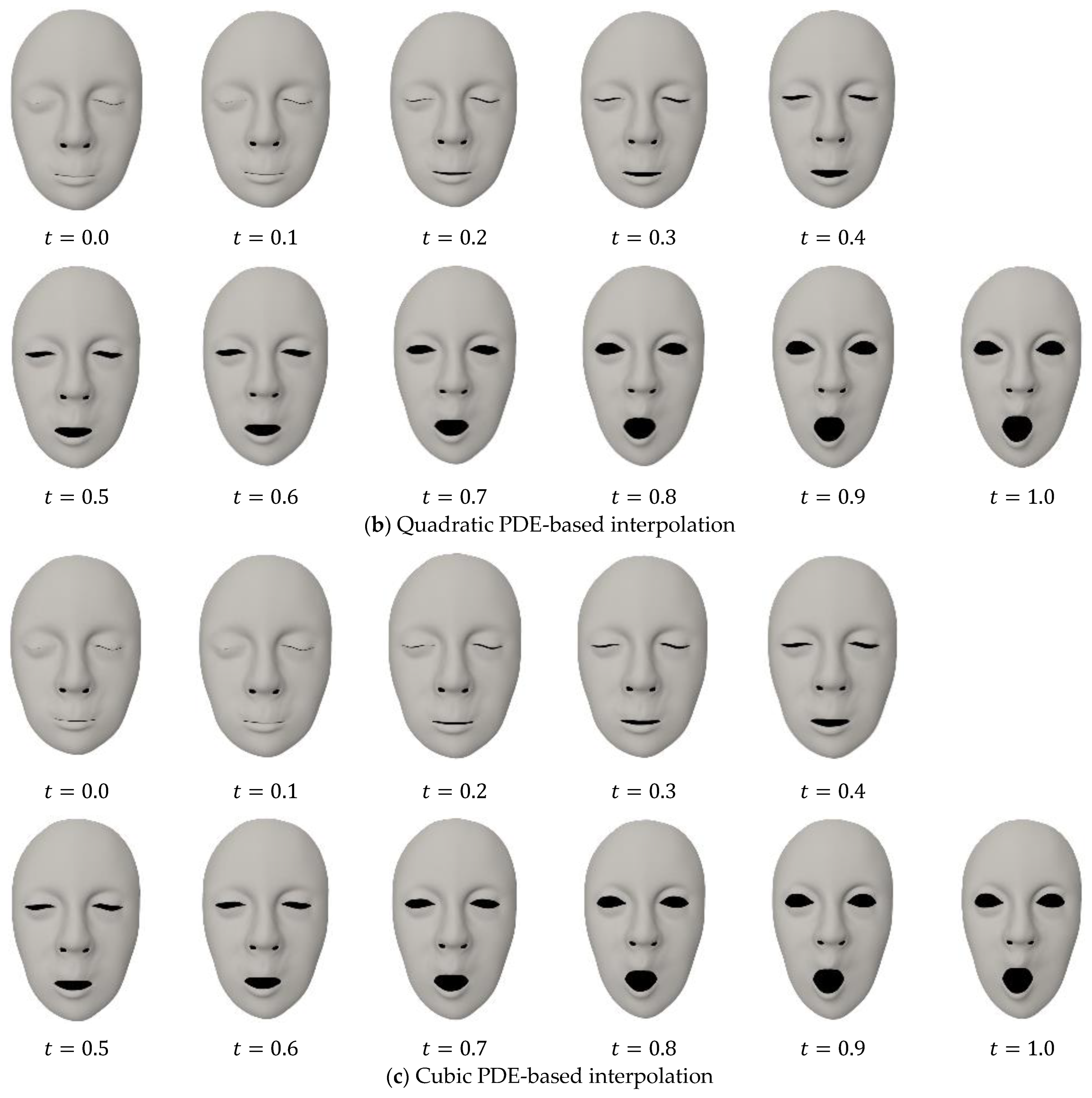
For PDE-based shape interpolation, $w_0\left(u\right)$ and $w_1\left(u\right)$ indicate the curves on the neutral model ($t=0.0$) and target model ($t=1.0$) shown in Figure 4, respectively. After substituting Equations (31)–(33) to determine the unknown constants, we use them to obtain the facial models by setting $t=0.1$, 0.2, 0.3, …, 0.9 in Equations (31)–(33) and depicted the obtained facial models in Figure 6 where Figure 6a–c are from Equations (31)–(33), respectively.

Substituting $w_{0n}$ obtained from the facial model at $t=0.0$ and $w_{1n}$ obtained from the facial model at $t=1.0$ shown in Figure 4 into the geometric linear interpolation (34) and setting $t$ to 0.1, 0.2, 0.3, …, 0.9, respectively, we obtain the facial models at the nine poses and depicted them in Figure 6d.

Comparing Figure 6 with Figure 4, we found that the quadratic PDE-based interpolation and cubic PDE-based interpolation create more realistic facial models than the geometric linear interpolation and linear PDE-based interpolation. The facial models created by the quadratic PDE-based interpolation and cubic PDE-based interpolation are the closest to the ground-truth models shown in Figure 4.

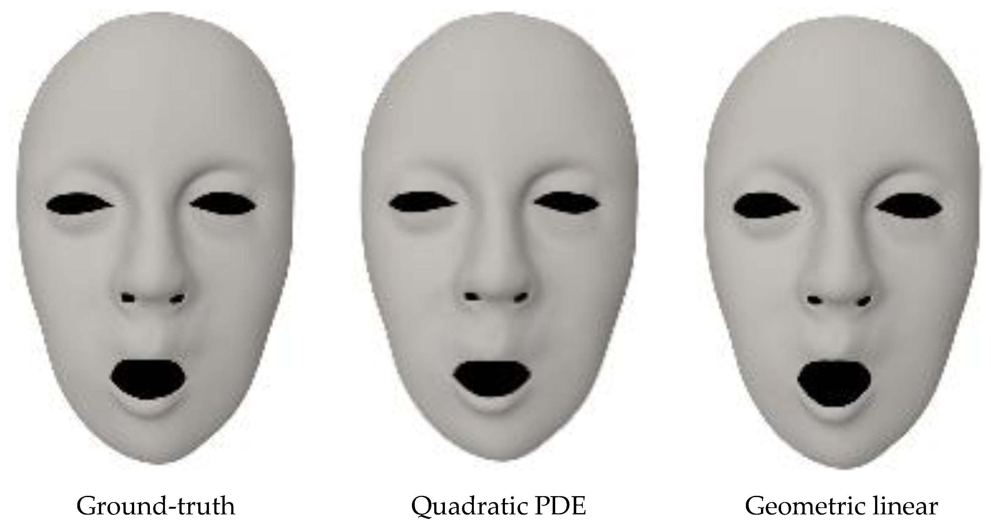
In order to show the differences between the ground-truth models and the models obtained with the quadratic PDE-based interpolation and the geometric linear interpolation more clearly, we put the models at $t=0.7$ in Figure 7 where the left, middle and right models are, respectively, from the ground-truth, quadratic PDE-based interpolation and the geometric linear interpolation. Observing the three models shown in Figure 7, it is clear that the model obtained with the quadratic PDE-based interpolation is far closer to the ground-truth model than the model obtained with the geometric linear interpolation.

To quantify the differences between the models created with different interpolation methods and the ground-truth models, we calculate the average and maximum errors of the corresponding curves on the created models and the ground-truth models with the following equations:

$$\begin{gathered} E_A=\frac{1}{N}{\sum }_{n=1}^N\frac{{\overline{w}}_{tn}-{\stackrel{̿}{w}}_{tn}}{D} \\ {E}_M=max\frac{1}{D}\left\{\begin{array}{ccc}{\overline{w}}_{t1}-{\stackrel{̿}{w}}_{t1}& {\overline{w}}_{t2}-{\stackrel{̿}{w}}_{t2}& \begin{array}{cc}\dots & {\overline{w}}_{tN}-{\stackrel{̿}{w}}_{tN}\end{array}\end{array}\right\} \end{gathered}$$

(35)

where the overbar indicates the ground-truth models, the double overbar indicates the created models, and $D$ is the distance between the two farthest vertices on the neutral model.

The obtained average errors $E_A$ and the maximum error $E_M$ are shown in the graphs of Figure 8. In the Figure, the numbers 1–49 on the horizontal axis are the index of the curves.

The largest maximum error and largest average error of the 49 curves are given in

Table 1. Largest maximum errors and largest average errors.

	Linear PDE	Quadratic PDE	Cubic PDE	Geometric Linear Interpolation
LME	0.021548	0.010629	0.010826	0.024761
LAE	0.009358	0.006903	0.007916	0.011378

, where LME stands for the largest maximum error, and LAE indicates the largest average error. The data in the table indicate the following: (1) all three PDE-based interpolation methods, i.e., linear PDE, quadratic PDE and cubic PDE achieve smaller values of the largest maximum error and largest average error than the geometric linear interpolation; (2) among the three PDE-based interpolation methods, the quadratic PDE-based interpolation achieves the smallest values of the largest maximum error and largest average error; (3) the largest maximum error and the largest average error caused by the geometric linear interpolation are 2.33 and 1.65 times of those caused by the quadratic PDE-based interpolation.

From Figure 6, Figure 7 and Figure 8 and the above discussions, we can conclude the following: (1) The average and maximum errors caused by the geometric linear interpolation are the largest except for the average errors for curves 21, 22, 24, and 26–29. (2) In comparison with the geometric linear interpolation and linear PDE-based interpolation, the quadratic and cubic PDE-based shape interpolation methods have smaller average errors except for curves 24–29 and smaller maximum errors for all 49 curves. It indicates that facial skin deformations are nonlinear. (3) The largest average error and largest maximum error caused by the quadratic PDE-based interpolation are lower than those caused by the cubic PDE-based interpolation, (4) the quadratic PDE-based interpolation achieves smaller average errors for all the curves and smaller maximum errors for most curves than the cubic PDE-based interpolation. Conclusions (3) and (4) indicate that the quadratic PDE-based interpolation is more accurate than the cubic PDE-based interpolation. Therefore, the quadratic PDE-based interpolation can be used to create the most realistic facial shapes among the four methods discussed in this paper.

Based on the above discussion, we will apply the quadratic PDE-based method in interpolation between a neutral model and target models and facial blendshapes among different facial expressions to create more realistic facial shape changes than using the geometric linear interpolation in the remaining parts of this paper.

Although the linear PDE-based facial interpolation has bigger errors than the quadratic and cubic PDE-based facial interpolation, it is applicable to situations where shape changes are linear. For very few curves, such as curves 24–29 shown in the second of Figure 8, the cubic PDE-based facial interpolation has smaller maximum errors than the quadratic PDE-based facial interpolation. It indicates that the cubic PDE-based method may be more suitable for these curves than the quadratic PDE-based method.

The approach proposed in this paper is also applicable to part of a curve and the curves in local regions of face models. This can be easily achieved by using $w_0\left(u\right)$ and $w_1\left(u\right)$ in Equation (4) to represent part of a curve and the curves in local regions of face models. With such a treatment, more realistic facial interpolation can be obtained.

4.4. Quadratic PDE-Based Interpolation of Facial Models

One neutral and five target expressions will be used in interpolation calculations to create new facial models and animation. The five target facial expressions are sad, angry, confused, grinning, and puff. The neutral expression is shown in the left column of Figure 9. The sad, angry, confused, grinning, and puff expressions are shown in the right column of the Figure.

The curves representing the neutral expression are taken to be $w_0\left(u\right)$ in Equation (4) and the corresponding ones on each of the sad, confused, grinning, and puff expressions are taken to be $w_1\left(u\right)$. After setting $t=0$ and $t=1$ in Equation (32) and substituting it into Equation (4) to determine the unknown constants, we use it to create new facial models at any instant.

Setting the time variable $t$ in Equation (32) to 0.2, 0.4, 0.6, and 0.8, we obtain new facial models at these instants and depict them in the second, third, fourth, and fifth columns of Figure 9. In the Figure, the first, second, third, fourth, and fifth rows indicate sad, angry, confused, grinning, and puff expressions, respectively.

5. PDE-Based Facial Blendshapes

Facial blendshapes based on the geometric linear interpolation are to create new facial models with one neutral model and more than one target model through the following weighted combination [2]:

$$\mathit{w}={\mathit{w}}_0+{\sum }_{j=1}^N{\xi }_j({\mathit{w}}_j-{\mathit{w}}_0)$$

(36)

where ${\mathit{w}}_0$ is a neutral model, ${\mathit{w}}_j$ ($j=1,2,3,\dots ,N$) are target models, and ${\xi }_j$ ($j=1,2,3,\dots ,N$) are weights with ${\xi }_j\ge 0$ and $\sum _{j=1}^N{\xi }_j=1$.

With the PDE-based interpolation proposed in this paper, we use Equation (32) to interpolate a neutral expression and the jth target expression and obtain the following quadratic PDE-based interpolation equation for the jth target expression:

$$\begin{gathered} \begin{array}{l}{w}^j(u, t)=b_{w0}^j+\left(\frac{{\overline{e}}_{w0}^j}{c}+\frac{{2m}^2{\stackrel{̿}{e}}_{w0}^j}{c^3}\right)t-\frac{m{\stackrel{̿}{e}}_{w0}^j}{c^2}{t}^2+{\stackrel{̿}{e}}_{w0}^j{t}^3/(3c)+\\ \hspace{1em}\hspace{1em}\hspace{1em}\hspace{1em}\hspace{1em}\hspace{1em}{\displaystyle \sum _{n=1}^N}[(\frac{{\widehat{e}}_{wn}^j}{B_n}-\frac{2m{\check{e}}_{wn}^j}{B_n^2}+\frac{{2c}^2}{B_n^3}{\check{e}}_{wn}^j-\frac{2c}{B_n^2}{\check{e}}_{wn}^{j}t+{\check{e}}_{wn}^j{t}^2/B_n)cos2n\pi u\\ \hspace{1em}\hspace{1em}\hspace{1em}\hspace{1em}\hspace{1em}\hspace{1em}+(\frac{{\tilde{e}}_{wn}^j}{B_n}-\frac{2m{\overline{e}}_{wn}^j}{B_n^2}+\frac{{2c}^2}{B_n^3}{\overline{e}}_{wn}^j-\frac{2c}{B_n^2}{\overline{e}}_{wn}^{j}t+{\overline{e}}_{wn}^j{t}^2/B_n)sin2n\pi u]\end{array} \\ (w=x, y, z) \end{gathered}$$

(37)

Substituting the above analytical solution into the following blending Equation

$$w^b\left(u, t\right)={\sum }_{j=1}^N{\xi }_j{w}^j(u, t) (w=x, y, z)$$

(38)

we obtain the following:

$$\begin{gathered} w^b(u, t)=b_{w0}^b+\left(\frac{{\overline{e}}_{w0}^b}{c}+\frac{{2m}^2{\stackrel{̿}{e}}_{w0}^b}{c^3}\right)t-\frac{m{\stackrel{̿}{e}}_{w0}^b}{c^2}{t}^2+{\stackrel{̿}{e}}_{w0}^b{t}^3/(3c) \\ +\sum _{n=1}^N\left[(\frac{{\widehat{e}}_{wn}^b}{B_n}-\frac{2m{\check{e}}_{wn}^b}{B_n^2}+\frac{{2c}^2}{B_n^3}{\check{e}}_{wn}^b-\frac{2c}{B_n^2}{\check{e}}_{wn}^{b}t+{\check{e}}_{wn}^b{t}^2/B_n)cos2n\pi u\right. \\ \left.+(\frac{{\tilde{e}}_{wn}^b}{B_n}-\frac{2m{\overline{e}}_{wn}^b}{B_n^2}+\frac{{2c}^2}{B_n^3}{\overline{e}}_{wn}^b-\frac{2c}{B_n^2}{\overline{e}}_{wn}^{b}t+{\overline{e}}_{wn}^b{t}^2/B_n)sin2n\pi u\right] \\ (w=x, y, z) \end{gathered}$$

(39)

where

$$\begin{gathered} b_{w0}^b={\sum }_{j=1}^N{\xi }_j{b}_{w0}^j \\ {\overline{e}}_{w0}^b={\sum }_{j=1}^N{\xi }_j{\overline{e}}_{w0}^j \\ {\stackrel{̿}{e}}_{w0}^b={\sum }_{j=1}^N{\xi }_j{\stackrel{̿}{e}}_{w0}^j \\ {\widehat{e}}_{wn}^b={\sum }_{j=1}^N{\xi }_j{\widehat{e}}_{wn}^j \\ {\check{e}}_{wn}^b={\sum }_{j=1}^N{\xi }_j{\check{e}}_{wn}^j \\ {\tilde{e}}_{wn}^b={\sum }_{j=1}^N{\xi }_j{\tilde{e}}_{wn}^j \\ {\overline{e}}_{wn}^b={\sum }_{j=1}^N{\xi }_j{\overline{e}}_{wn}^j \end{gathered}$$

(40)

For the neutral expressions and the sad, angry, confused, grinning, and puff expressions investigated in the above section, we have $N=5$. Respectively setting the weights ${\xi }_j$ and the time variable $t$ to different values, we can use Equations (39) and (40) to create many new blend shapes.

For the illustrative purpose, we set ${\xi }_j$ to 0.0, 0.2, 0.4, 0.6, 0.8, and 1.0 for each of the analytical solutions obtained from the five target expressions. It gives 7775 different weight combinations. For example, ${\xi }_1=0.2$, ${\xi }_2=0.0$, ${\xi }_3=0.6$, ${\xi }_4=1.0$, and ${\xi }_5=0.8$ are one weight combinations. The sum of these weights is larger than 1.0. They can be scaled to satisfy the sum of 1.0 through ${\xi }_j/{\sum }_i^5{\xi }_i$ ($i=1, 2, 3, 4, 5$), i.e., ${\xi }_1=0.0769$, ${\xi }_2=0.0$, ${\xi }_3=0.2308$, ${\xi }_4=0.3846$, and ${\xi }_5=0.3077$.

For each of the weight combinations, we set the time variable $t$ to different instants and substitute them into Equation (39) to obtain the facial models at the instants. Here, we set $t=1.0$ and use the 7775 weight combinations to obtain 7775 new facial models. Figure 10 below shows 50 facial models selected from the 7775 facial models.

The above figure shows that different combinations of facial blendshape weights create different shapes when the time variable $t$ is fixed. Different from the facial blendshapes using Equation (36), where one weight combination can create one new shape only, the facial blendshapes using Equation (39) will enable one weight combination to create many different new shapes by simply setting the time variable $t$ to different values. It indicates that the proposed method not only improves the realism of facial interpolation and facial blendshapes but also noticeably raises the capacity to create more facial shapes for facial animation.

We have calculated the CPU time using the quadratic PDE-based facial blendshapes to obtain the coordinate values of the 259 and 7775 facial models with 5071 vertices for each of the facial models. On a laptop with a 3.3 GHz Intel Core i7- processor and 16 GB of main memory, it takes 2.46 s to create the 259 facial models and 72.748 s to create the 7779 facial models. In [20], physics-based simulation is used to consider the physical interaction of passive flesh, active muscles, and rigid bone structures, and the numerical solution takes over 2 min to generate a new facial model with 6393 surface vertices and 8098 volumetric vertices on a laptop with a 3.1 GHz Intel Core i7 processor and 16 GB of main memory. Clearly, the analytical PDE-based approach proposed in this paper is far more efficient than the numerical method proposed in [20].

Apart from the advantage of the high efficiency of the quadratic PDE-based facial blendshapes, another advantage is good realism. Since the quadratic PDE-based interpolation Equation (32) creates the most realistic shapes among the geometric linear interpolation and the three PDE-based interpolation methods based on Equations (31)–(33), the facial blendshapes based on the quadratic PDE-based interpolation Equation (32) are more realistic than the facial blendshapes based on the geometric linear interpolation and the linear and cubic PDE-based shape interpolation.

6. Conclusions

How to create new and realistic facial expressions efficiently from two known facial expressions is an important and unsolved problem. In this paper, we have developed a new facial interpolation method to tackle the problem and used the new facial interpolation method to develop a new method of facial blendshapes.

The new facial interpolation and blendshape approach is physics-based and analytical, which simulates dynamic skin deformation with better realism than the methods based on geometric linear interpolation and higher simulation efficiency than numerical physics-based techniques. To develop the new approach, we have converted the polygon representation of three-dimensional facial models into a curve representation, introduced curve deformation resistance into the equation of motion and combined it with the boundary conditions of curve shape changes to obtain the mathematical model of facial skin deformations, derived analytical solutions of the mathematical model, and used them to achieve linear and nonlinear physics-based interpolation and blendshapes of facial models.

We have compared the ground-truth facial shape changes to those obtained from the proposed approach and the geometric linear interpolation and demonstrated that the proposed approach achieves better realism of facial shape interpolation than the geometric linear interpolation. Due to the nature of the analytical solutions of the physics-based mathematical model, the proposed approach is far more efficient than existing numerical solutions of physics-based models.

References

- Liu, X.; Xia, S.; Fan, Y.; Wang, Z. Exploring non-linear relationship of blendshape facial animation. Comput. Graph. Forum 2011, 30, 1655–1666. [Google Scholar] [CrossRef]
- Lewis, J.P.; Anjyo, K.; Rhee, T.; Zhang, M.; Pighin, F.H.; Deng, Z. Practice and theory of blendshape facial models. In Proceedings of the Eurographics 2014—State of the Art Reports, Strasbourg, France, 7–11 April 2014; pp. 199–218. [Google Scholar]
- Pighin, F.; Hecker, J.; Lischinski, D.; Szeliski, R.; Salesin, D.H. Synthesizing realistic facial expressions from photographs. In Proceedings of the SIGGRAPH 25th Annual Conference on Computer Graphics and Interactive Techniques, Orlando, FL, USA, 19–24 July 1998; pp. 75–84. [Google Scholar]
- Alkawaz, M.H.; Mohamad, D.; Basori, A.H.; Saba, T. Blend shape interpolation and FACS for realistic avatar. 3D Res. 2015, 6, 6. [Google Scholar] [CrossRef]
- Waters, K.; Levergood, T.M. Decface: An automatic lip-synchronization algorithm for synthetic faces. In Proceedings of the Second ACM International Conference on Multimedia, San Francisco, CA, USA, 15–20 October 1994; pp. 149–156. [Google Scholar]
- Lewis, J.P.; Anjyo, K.-I. Direct manipulation blendshapes. IEEE Comput. Graph. Appl. 2010, 30, 42–50. [Google Scholar] [CrossRef]
- Li, H.; Weise, T.; Pauly, M. Example-based facial rigging. ACM Trans. Graph. 2010, 29, 1–6. [Google Scholar]
- Yu, H.; Liu, H. Regression-based facial expression optimization. IEEE Trans. Hum. Mach. Syst. 2014, 44, 386–394. [Google Scholar]
- Han, J.H.; Kim, J.I.; Suh, J.W.; Kim, H. Customizing blendshapes to capture facial details. J. Supercomput. 2023, 79, 6347–6372. [Google Scholar] [CrossRef]
- Racković, S.; Soares, C.; Jakovetić, D.; Desnica, Z.; Ljubobratović, R. Clustering of the blendshape facial model. In Proceedings of the 29th European Signal Processing Conference, Dublin, Ireland, 23–27 August 2021; pp. 1556–1560. [Google Scholar]
- Diego, M.; Claudio, E.; Ricardo, M. Laplacian face blending. Comput. Animat. Virtual Worlds 2023, 34, e2044. [Google Scholar]
- Tenenbaum, J.B.; Freeman, W.T. Separating style and content with bilinear models. Neural Comput. 2000, 12, 1247–1283. [Google Scholar] [CrossRef]
- Mpiperis, I.; Malassiotis, S.; Strintzis, M.G. Bilinear models for 3D face and facial expression recognition. IEEE Trans. Inf. Forensics Secur. 2008, 3, 498–511. [Google Scholar] [CrossRef]
- Vlasic, D.; Brand, M.; Pfister, H.; Popović, J. Face transfer with multilinear models. ACM Trans. Graph. 2005, 24, 426–433. [Google Scholar] [CrossRef]
- Roh, J.H.; Kim, S.U.; Jang, H.; Seol, Y.; Kim, J. Interactive facial expression editing with non-linear blendshape interpolation. In Proceedings of the Eurographics, Reims, France, 25–29 April 2022; pp. 69–72. [Google Scholar]
- Ma, W.C.; Wang, Y.H.; Fyffe, G.; Barbič, J.; Chen, B.Y.; Debevec, P. A blendshape model that incorporates physical interaction. Comput. Animat. Virtual Worlds 2012, 23, 235–243. [Google Scholar] [CrossRef]
- Hahn, F.; Martin, S.; Thomaszewski, B.; Sumner, R.; Coros, S.; Gross, M. Rig-space physics. ACM Trans. Graph. 2012, 31, 1–8. [Google Scholar] [CrossRef]
- Barrielle, V.; Stoiber, N.; Caqniart, C. Blendforces: A dynamic framework for facial animation. Comput. Graph. Forum. 2016, 35, 341–352. [Google Scholar] [CrossRef]
- Kozlov, Y.; Bradley, D.; Bächer, M.; Thomaszewski, B.; Beeler, T.; Gross, M. Enhancing facial blendshape rigs with physical simulation. Comput. Graph. Forum. 2017, 36, 75–84. [Google Scholar] [CrossRef]
- Ichim, A.-E.; Kadleček, P.; Kavan, L.; Pauly, M. Phace: Physics-based face modelling and animation. ACM Trans. Graph. 2017, 36, 1–14. [Google Scholar] [CrossRef]
- Wagner, N.; Schwanecke, U.; Botsch, M. Neural Volumetric Blendshapes: Computationally Efficient Physics-Based Facial Blendshapes. 2023. Available online: https://arxiv.org/pdf/2212.14784.pdf (accessed on 10 November 2023).
- Bloor, M.I.G.; Wilson, M.J. Using partial differential equations to generate free-form surfaces. CAD 1990, 22, 202–212. [Google Scholar] [CrossRef]
- Ugail, H.; Bloor, M.I.G.; Wilson, M.J. Techniques for interactive design using the PDE method. ACM Trans. Graph. 1999, 18, 195–212. [Google Scholar] [CrossRef]
- Monterde, J.; Ugail, H. A general 4th-order PDE method to generate Bézier surfaces from the boundary. CAGD 2006, 23, 208–225. [Google Scholar] [CrossRef]
- Xu, G.; Zhang, Q. A general framework for surface modeling using geometric partial differential equations. CAGD 2008, 25, 181–202. [Google Scholar] [CrossRef]
- You, L.H.; Yang, X.S.; Zhang, J.J. Dynamic skin deformation with characteristic curves. Comp. Anim. Virtual Worlds 2008, 19, 433–444. [Google Scholar] [CrossRef]
- Castro, G.G.; Ugail, H.; Willis, P.; Palmer, I. A survey of partial differential equations in geometric design. Vis. Comput. 2008, 24, 213–225. [Google Scholar] [CrossRef]
- Sheng, Y.; Sourin, A.; Castro, G.G.; Ugail, H. A PDE method for patchwise approximation of large polygon meshes. Vis. Comput. 2010, 26, 975–984. [Google Scholar] [CrossRef]
- Ugail, H. Partial Differential Equations for Geometric Design; Springer: Berlin/Heidelberg, Germany, 2011; ISBN 978-0-85729-783-9. [Google Scholar]
- Sheng, Y.; Willis, P.; Castro, G.G.; Ugail, H. Facial geometry parameterisation based on partial differential equations. Math. Comput. Model. 2011, 54, 1536–1548. [Google Scholar] [CrossRef]
- Pan, Q.; Xu, G.; Zhang, Y. A unified method for hybrid subdivision surface design using geometric partial differential equations. CAD 2014, 46, 110–119. [Google Scholar] [CrossRef]
- Chen, C.; Sheng, Y.; Li, F.; Zhang, G.; Ugail, H. A PDE-based head visualization method with CT data. Comp. Anim. Virtual Worlds 2017, 28, e1683. [Google Scholar] [CrossRef]
- Wang, S.B.; Xia, Y.; Wang, R.; You, L.H.; Zhang, J.J. Optimal NURBS conversion of PDE surface-represented high-speed train heads. Optim. Eng. 2019, 20, 907–928. [Google Scholar] [CrossRef]
- You, L.H.; Yang, X.S.; Pan, J.J.; Bian, S.J.; Qian, K.; Habib, Z.; Sargano, A.B.; Kazmi, I.; Zhang, J.J. Fast character modeling with sketch-based PDE surfaces. Multimed. Tools Appl. 2020, 79, 23161–23187. [Google Scholar] [CrossRef]
- Wang, S.B.; Xia, Y.; You, L.H.; Ugail, H.; Carriazo, A.; Iglesias, A.; Zhang, J.J. Interactive PDE patch-based surface modeling from vertex-frames. Eng. Comput. 2022, 38, 4367–4385. [Google Scholar]
- Zhu, Z.; Iglesias, A.; Zhou, L.; You, L.H.; Zhang, J.J. PDE-based 3D surface reconstruction from multi-view 2D images. Mathematics 2022, 10, 542. [Google Scholar] [CrossRef]
- Fu, H.B.; Bian, S.J.; Chaudhry, E.; Wang, S.B.; You, L.H.; Zhang, J.J. PDE surface-represented facial blendshapes. Mathematics 2021, 9, 2905. [Google Scholar] [CrossRef]
- Terzopoulos, D.; Waters, K. Analysis and synthesis of facial image sequences using physical and anatomical models. IEEE Trans. Pattern Anal. Mach. Intell. 1993, 15, 569–579. [Google Scholar] [CrossRef]
- Lee, Y.; Terzopoulos, D.; Waters, K. Realistic modeling for facial animation. In Proceedings of the 22nd Annual Conference on Computer Graphics and Interactive Techniques, Los Angeles, CA, USA, 6–11 August 1995; pp. 55–62. [Google Scholar]
- Warburton, M.; Maddock, S. Physically-based forehead animation including wrinkles. Comp. Anim. Virtual Worlds 2013, 26, 55–68. [Google Scholar] [CrossRef]
- Park, S.I.; Hodgins, J.K. Data-driven modelling of skin and muscle deformation. ACM Trans. Graph. 2008, 27, 1–6. [Google Scholar]
- Kakadiaris, I.A. Physics-Based Modeling, Analysis and Animation; Technical Reports No. MS-CIS-93-45; University of Pennsylvania: Philadelphia, PA, USA, 1993. [Google Scholar]
- Kadleček, P.; Ichim, A.-E.; Liu, T.; Křivánek, J.; Kavan, L. Reconstructing personalised anatomical models for physics-based body animation. ACM Trans. Graph. 2016, 35, 1–13. [Google Scholar] [CrossRef]
- Schönberger, J.L.; Frahms, J.-M. Structure-from-Motion revisited. In Proceedings of the Conference on Computer Vision and Pattern Recognition (CVPR), Las Vegas, NV, USA, 27–30 June 2016; pp. 4104–4113. [Google Scholar]
- Schönberger, J.L.; Zheng, E.; Pollefeys, M.; Frahm, J.-M. Pixelwise view selection for unstructured multi-view stereo. In Proceedings of the European Conference on Computer Vision (ECCV), Amsterdam, The Netherlands, 11–14 October 2016; pp. 501–518. [Google Scholar]