

Approximate and Parametric Solutions to SIR Epidemic Model


1
Department of Mathematics, Faculty of Science, Imam Mohammad Ibn Saud Islamic University (IMSIU), Riyadh 11623, Saudi Arabia
2
Department of Physics, Faculty of Science, Imam Mohammad Ibn Saud Islamic University (IMSIU), Riyadh 11623, Saudi Arabia
3
Department of Mathematics and Sciences, Prince Sultan University, Riyadh 11586, Saudi Arabia
*
Author to whom correspondence should be addressed.
Axioms 2024, 13(3), 201; https://doi.org/10.3390/axioms13030201
Submission received: 25 January 2024
/
Revised: 25 February 2024
/
Accepted: 14 March 2024
/
Published: 16 March 2024
(This article belongs to the Special Issue Infinite Dynamical System and Differential Equations)
Abstract
:This article provides a detailed exploration of the SIR epidemic model, starting with its meticulous formulation. The study employs a novel approach called the upper and lower bounds technique to approximate the solution to the SIR model, providing insights into the dynamic interplay between susceptible S, infected I, and recovered R populations. A new parametric solution to this model has been presented. Applying the Adomian decomposition method (ADM) allows for the attaining of highly accurate approximate solutions in the context of the SIR epidemic model. To validate the accuracy and robustness of the proposed approach, a numerical exploration is conducted, considering a diverse range of experimental parameters. This numerical analysis provides valuable insights into the sensitivity and responsiveness of the SIR epidemic model under varying conditions, contributing to the broader understanding of infectious disease dynamics. The interplay between theoretical formulation and numerical exploration establishes a comprehensive framework for studying the SIR model, with implications for refining our ability to predict and manage the spread of infectious diseases.
Keywords:
SIR epidemic model; upper bound of solution; lower bound of solution; solution in parametric form; Adomian decomposition methodMSC:
39A27; 65L10; 34L15; 49M271. Introduction
The SIR epidemic model provides a rigorous framework for understanding the temporal evolution of a population’s susceptibility S, infection I, and recovery R to time t. This model is described by a set of non-linear ordinary differential equations, as presented in Equation (1) [1,2]:
These equations encapsulate the dynamics of I, and R populations, with the initial conditions outlined in Equation (2):
where and are non-negative constant parameters. The equation describing the behavior of R evolves from the infected population I, expressed as
The SIR (Susceptible-Infectious-Removed) model is a fundamental and significant epidemiological model due to its simplicity, clarity, and historical importance. Although more complex and modern models [3,4,5,6,7,8], have been developed to address specific small differences in infectious disease dynamics, the SIR model remains valuable. The choice of model depends on analysis objectives and the level of detail needed.
A substantial body of literature has been dedicated to numerical methods for solving these equations, such as the homotopy analysis method (HAM) [9]. Recently, in [10], the authors explored this coupled non-linear system and introduced an approximate solution through asymptotic approximants.
This paper is devoted to finding the new upper and lower bounds of solutions to this SIR epidemic model in explicit forms. Further, finding lower and upper bounds for solutions to differential equations is an important mathematical and analytical tool. It can provide insights, validation, and practical benefits in understanding and modeling various physical and engineering systems. These bounds help to characterize the behavior and limitations of the system under study.
It is often challenging, if possible, to find explicit solutions to some systems. However, converting such a system to an equivalent second-order nonlinear differential equation can help in finding solutions in parametric form. As a result, a new solution in parametric form can be provided.
Overall, the Adomian decomposition method (ADM) [11,12,13,14,15,16,17,18,19,20,21,22,23] is a powerful analytical method for approximating solutions to the SIR epidemic model, contributing significantly to understanding disease dynamics and informing public health strategies. The ADM provides an analytical framework that offers closed-form or series solutions, which helps in obtaining analytical expressions for the SIR model’s behavior over time. Moreover, the ADM allows for the handling of nonlinear differential equations, enabling the study of complex epidemic models that often exhibit nonlinear dynamics and providing a more realistic representation of disease spread. The ADM can yield accurate solutions, particularly for problems with known or expected smooth solutions, contributing to a precise understanding of epidemic behavior and dynamics. Therefore, we use the ADM to find excellent approximation solutions for the SIR epidemic model concerning real scenarios. Results obtained from the Adomian method are compared with numerical solutions, providing validation and a better understanding of the model’s behavior.
2. Solutions to System (1)–(3)
We first begin by converting system (1) and (2) to an equivalent system through the following transformations:
2.1. Upper and Lower Bounds of Solutions
The following fundamental lemma is an important tool in finding the upper and lower bounds of system solutions (1)–(3).
Lemma 1.
The following system,
can be converted into an equivalent first-order nonlinear equation in u,
where is a constant of integration.
Proof.
Differentiating the first equation of Equation (6) with respect to we obtain
We now rewrite Equation (7) in the form
where with
Now, using the well-known exponential inequality , we get
that is,
where
For comparison purposes, we have the following initial-value problem for the linear equation:
The solution to w is then easy:
Since is continuous in t and w and Lipschitz in w, we can apply the comparison theorem to Equation (11) with to get
Consequently,
which is the lower bound of
To now find the lower bound of from the system (5), we take the second equation:
In view of this and since we obtain
A simple integration from 0 to t leads to
Hence,
Consequently,
It remains, therefore, only to find the upper bounds of S and In finding them, we shall make use of Equations (1). Indeed, from the first equation of Equations (1),
and in view of (22), we obtain
It follows that
or
A simple integration again from 0 to t gives us
or
where
Thus, we have proven the following:
2.2. Solutions in Parametric Forms
The following lemma is also an important tool in finding solutions in parametric forms to system (1)–(3).
Lemma 2.
System (6) can be also converted into an equivalent second-order nonlinear equation in v
Proof.
Differentiating the second equation of (6) with respect to we obtain
We rewrite Equation (41) as follows:
Setting gives
The substitution leads to
Thus, the solution to this second-order nonlinear equation in the unknown in parametric form is given by (Section 2.7.3-2 in [24]):
where and are constants of integration.
We have the following:
Theorem 2.
The solution in parametric form is given by
where
3. Analytic Approximate Solutions via Adomian Decomposition Method
We propose here to solve (5) using the Adomian decomposition method (ADM) [11,12,13,14,15,16,17,18,19,20,21,22,23].
First, we define the linear operator nonlinear operator N, and inverse linear operator as
We rewrite (5) in Adomian’s operator-theoretic notation as
Upon substitution, we have
Using the classic Adomian decomposition method, we decompose the solution into the solution components to be determined via recursion and the nonlinearity into the corresponding Adomian polynomials tailored to the particular nonlinearity as
where the first few Adomian polynomials [11,12] are given in the Appendix A.
Upon substitution, we obtain
Then, we establish the Adomian recursion scheme as
The first few components of the solution are given by
Hence,
Attaining a satisfactory approximate solution for will enable the determination of and using Equations (5) and (3), respectively. Notably, deriving from the second equation within system (5), we obtain
Integrating this equation from 0 to t, we obtain
Then,
and
It is important to note that when using the Adomian method, certain considerations must be taken into account. Indeed, the Adomian decomposition method is a precious tool for analyzing the SIR model, offering a systematic, analytical, and interpretable solution that significantly improves our understanding of infectious disease dynamics. It is imperative to thoroughly examine the convergence of the ADM series.
3.1. Convergence Analysis
3.1.1. Uniqueness Theorem
We can obtain a uniqueness theorem to this system beginning with the initial-value problem of Equation (7) with
Since has which is not bounded, f is not Lipschitzian. If we assume that there is a solution u to this initial-value problem which remains in , then, in the restricted region we have
Applying the Mean Value Theorem to the function , we obtain
Thus,
Hence, is Lipschitzian with
Assuming that and are two different solutions to this initial-value problem,
Using Gronwall’s inequality, we obtain Thus,
Hence, the solution u to this initial-value problem exists and is unique. In view of this, we conclude that the solution to (6) exists and is unique.
Consequently,
Theorem 3.
The SIR epidemic model has only one solution
3.1.2. Convergence Theorem
The series solution obtained using the ADM converges with rapidity, and successive terms are easily computed. For the proof of the convergence of Adomian’s method, we refer to the useful reference [25], in which Cherruault [25] proposed an interesting technique to prove the convergence under suitable and reasonable hypotheses for the numerical resolution of nonlinear equations. To examine this convergence, let us take the initial-value problem of Equation (7) with which is equivalent to the above system (50). For every convergent series we define so that
The Adomian technique is equivalent to determine the sequences [25]:
A simple computation leads to
Let be a Banach space of all continuous functions on with norm where Consider the sequence of partial sums with Thus,
Hence,
Use and to get
Since N is Lipschitzian with
Similar arguments can be applied as in [26] to show that is a Cauchy sequence in
Thus,
Theorem 4.
The series solution for the initial-value problem of Equation (7) with obtained via the ADM converging if and
4. Numerical Explorations and Analysis
In the beginning, we will investigate the numerical solutions to the SIR epidemic model (1) and (3) with the initial conditions (2) using the numerical solution using a Fehlberg fourth-fifth order Runge–Kutta method with a degree-four interpolant [27,28,29,30]. This method is also known as the Runge–Kutta–Fehlberg (RKF45) method and offers several advantages over traditional fixed-step methods like the standard fourth-order Runge–Kutta method. Indeed, solving ordinary differential equations using numerical methods is advantageous due to its adaptivity, higher accuracy, efficient error estimation, versatility, and widespread applicability.
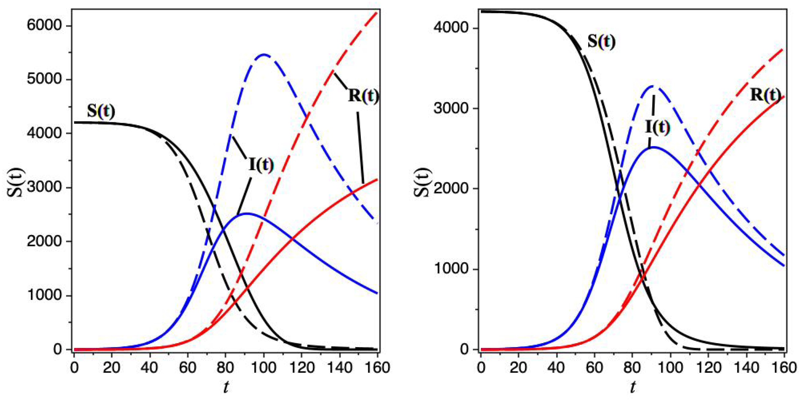
In Figure 1, we present the numerical solutions to the SIR epidemic model (1) and (3) with the initial conditions (2). Left panel: . Mid panel: . Right panel: . These initial conditions and the values of the parameters of the system are well-chosen from [9,10], which are excellent cases with the SIR epidemic model.
Here, we emphasize the essential point that is an essential property of the SIR model. The “positivity property” is a key concept in epidemiological modeling. It refers to the fact that variables like the number of individuals in different compartments, such as those who are susceptible, infected, or recovered, cannot be negative. This is because, in the context of infectious disease dynamics, it is impossible to have a negative number of individuals in any of these compartments. Therefore, the positivity property is an essential characteristic that must be considered when modeling the spread of infectious diseases.
Certainly, we observe from Equations (1)–(3) that , establishing , where N represents the total population. It can be straightforwardly demonstrated that and [2]. Furthermore, the essential characteristic is demonstrated in the numerical results illustrated in Figure 1.
Conversely, in Figure 2, we present the parametric solutions to the SIR epidemic model for the initial conditions . The parametric solutions to the SIR epidemic model offer several advantages in understanding and analyzing the dynamics of infectious diseases. In essence, parametric solutions to the SIR epidemic model facilitate a comprehensive understanding of infectious disease dynamics, providing insights into how different factors influence the spread and control of diseases and aiding in the development of effective public health strategies.
In addition, to explore the finding of a good approximation for the SIR epidemic model, we suggest a useful, powerful technique that is called the Adomian decomposition method (ADM), which is used to solve nonlinear ordinary and partial differential equations. Its advantages lie in its simplicity, efficiency, and applicability to a wide range of nonlinear problems. However, the application of the ADM to the SIR epidemic model provides robust approximate solutions. Specifically, the method decomposes the nonlinear differential equations governing the dynamics of susceptible S, infected I, and recovered R populations into a series of functions. This decomposition enables the iterative solution of each constituent. In the context of the SIR model’s nonlinear differential equations representing the changing rates of , and R populations, ADM effectively breaks down these equations into a series of functions. This breakdown allows for the step-by-step determination of individual terms within the solution series. Meanwhile, it is essential to consider the reduction in numerical volume and the swift convergence of the approximate solutions for further progress. Our suggestion to employ the ADM technique that accounts for these factors is crucial for effective progress. The iterative process of the ADM involves computing Adomian polynomials and their associated coefficients. This computation method generates an approximate solution, which can be refined by including additional terms in the series expansion. Utilizing ADM facilitates the acquisition of an analytical approximation for the solution to the SIR epidemic model. This analytical approximation proves instrumental in comprehending disease dynamics, predicting its behavior under diverse conditions, and evaluating the effects of interventions or parameter variations on the transmission of infectious diseases.
In Figure 3, we present a comparison between the numerical solutions to the SIR epidemic model with the fourth order of the solutions that are obtained using the ADM techniques for the initial conditions with the parameters [9,10]. The visual representation is delineated as follows: the dashed blue line depicts the numerical solution, the dotted black line illustrates the third-order solution derived using ADM, and the solid red line represents the fourth-order approximation attained through the ADM technique. The evident observation reveals a remarkable concurrence between the numerical solution and the fourth-order solutions obtained through the ADM technique for the function . There is appropriate agreement with numerical and fourth-order solutions by the ADM for the and functions.
In Figure 4, we present a comparison between the numerical solutions to the SIR epidemic model with the fifth order of the solutions that are obtained using the ADM techniques for the initial conditions with the parameters , which involve a scenario studied by Khan et al. [9,10] to simulate the 1966 bubonic plague outbreak in Eyam, England [9,10]. The figure displays the numerical solution as solid lines and the fifth-order solution obtained using the ADM technique as dashed lines. S, I, and R correspond to the black, blue, and red lines, respectively. Upon careful observation, it is evident that there is a significant agreement between the numerical solution and the fifth-order solutions obtained through the ADM technique for the functions at small values of t. For large values of t in months, numerical and fifth-order solutions obtained through the ADM for the functions have an appropriate agreement. The solutions are given in units of people. The right panel demonstrates a flawless alignment between the numerical solutions and the sixth-order solutions achieved through ADM. This highlights a significant advantage wherein ADM, even with lower orders of decomposition, can achieve remarkable agreement with the numerical solutions.
Figure 5 showcases a comparative analysis between the numerical solutions to the SIR epidemic model and the sixth-order solutions obtained using the ADM techniques. This evaluation pertains to specific initial conditions: , combined with the parameters and . In the left panel, a comparison between the seventh-order solutions obtained through the ADM and the numerical solutions reveals a notable discrepancy at larger time values, whereas, in the right panel, employing the eighth-order ADM solutions notably enhances the agreement. It should be noted that this scenario is a reference to a study conducted on the COVID-19 outbreak in Japan [10,31]. A slight increase in the order of decomposition in the ADM demonstrates improved concordance between numerical solutions and those derived via the ADM method. The ADM technique offers a valuable approach that delivers a strong approximation for the SIR epidemic model using lower-order decompositions, contrasting with other methods necessitating higher-order series expansions [10]. By increasing the order of decomposition, we can effectively handle situations where both and r are small. This approach ensures that we maintain the required level of accuracy in our results.
The proposed technique, which is directly stated, is said to offer a more efficient approach. This suggests that the proposed method can provide a solution of comparable quality while requiring fewer terms in the series expansion. This efficiency could have practical implications, such as reducing computational resources, simplifying calculations, or speeding up the modeling process. In essence, this point emphasizes the efficiency and effectiveness of the proposed technique in obtaining accurate solutions to the SIR model while streamlining the computational demands associated with other referenced methods [10]. On the other hand, the positive property persists in all the obtained results (Figure 3, Figure 4 and Figure 5).
Further, by comparing the results obtained through the ADM with numerical solutions, we can gain valuable insights into the convergence behavior. If the ADM solutions closely match the numerical solutions for a variety of scenarios, it indicates that the convergence is favorable. This information can be instrumental in improving the accuracy and reliability of the ADM model.
5. Conclusions
In conclusion, this research offers a comprehensive examination of the SIR epidemic model, delving into its meticulous formulation and employing innovative methodologies. The upper and lower bounds technique provides valuable insights into the interactions among susceptible, infected, and recovered populations and contributes to enhancing our theoretical comprehension through the derivation of an existence and uniqueness theorem. Moreover, applying the Adomian decomposition method demonstrates its effectiveness in yielding highly accurate approximate solutions to the SIR model.
Furthermore, the validation process, which involves numerical exploration across diverse experimental parameters, underscores the proposed approach’s accuracy and robustness. This numerical analysis sheds light on the SIR model’s sensitivity and adaptability under varying conditions, enriching our broader comprehension of infectious disease dynamics.
The suggested techniques explicitly highlight the useful efficiency, implying that it can provide an accurate satisfactory solution while utilizing fewer terms of the series expansion in the ADM method. This efficiency could have significant practical applications such as reducing the demand for computational resources, streamlining calculations, and expediting the modeling process.
This study has created a strong framework for studying the SIR model by combining theoretical formulation with numerical exploration. The findings of this study have significant implications for enhancing our predictive capabilities and improving strategies to manage and reduce the transmission of infectious diseases effectively.
Author Contributions
Conceptualization, L.B., S.B. and A.K.; methodology, L.B., A.K. and S.B.; software, S.B.; validation, L.B., A.K. and S.B.; formal analysis, A.K., L.B. and S.B.; investigation, A.K., L.B. and S.B.; writing original draft preparation, L.B., A.K. and S.B.; writing review and editing, A.K., L.B. and S.B. All authors have read and agreed to the published version of the manuscript.
Funding
This work was supported and funded by the Deanship of Scientific Research at Imam Mohammad Ibn Saud Islamic University (IMSIU) (grant number IMSIU-RG23018).
Institutional Review Board Statement
Not applicable.
Informed Consent Statement
Not applicable.
Data Availability Statement
This paper focuses on theoretical analysis and does not involve experiments and data.
Conflicts of Interest
The authors declare no conflicts of interest.
Appendix A. List of the Adomian Polynomials Ai for N(u) = eu [11,12,13]
The Adomian polynomials of for can be obtained in a similar form by using the functions instead of .
References
- Kermack, W.O.; McKendrick, A.G. A contribution to the mathematical theory of epidemics. Proc. R. Soc. Lond. Ser. A 1927, 115, 700–721. [Google Scholar]
- Bacaër, N. A Short History of Mathematical Population Dynamics; Springer: London, UK, 2011. [Google Scholar]
- Yin, Z.; Yu, Y.; Lu, Z. Stability analysis of an age-structured SEIRS model with time delay. Mathematics 2020, 8, 455. [Google Scholar] [CrossRef]
- Janssen, M.A.; Ostrom, E. Empirically based, agent-based models. Ecol. Soc. 2006, 11, 37. [Google Scholar] [CrossRef]
- Mollalo, A.; Vahedi, B.; Rivera, K.M. GIS-based spatial modeling of COVID-19 incidence rate in the continental United States. Sci. Total Environ. 2020, 728, 138884. [Google Scholar] [CrossRef]
- Sporns, O. Contributions and challenges for network models in cognitive neuroscience. Nat. Neurosci. 2014, 17, 652–660. [Google Scholar] [CrossRef] [PubMed]
- Sun, J.; Chen, X.; Zhang, Z.; Lai, S.; Zhao, B.; Liu, H.; Wang, S.; Huan, W.; Zhao, R.; Ng, M.T.A.; et al. Forecasting the long-term trend of COVID-19 epidemic using a dynamic model. Sci. Rep. 2020, 10, 21122. [Google Scholar] [CrossRef]
- Raval, M.; Sivashanmugam, P.; Pham, V.; Gohel, H.; Kaushik, A.; Wan, Y. Automated predictive analytics tool for rainfall forecasting. Sci. Rep. 2021, 11, 17704. [Google Scholar] [CrossRef] [PubMed]
- Khan, H.; Mohapatra, R.N.; Vajravelu, K.; Liao, S.J. The explicit series solution of SIR and SIS epidemic models. Appl. Math. Comput. 2009, 215, 653. [Google Scholar] [CrossRef]
- Barlow, N.S.; Weinstein, S.J. Accurate closed-form solution of the SIR epidemic model. Physica D 2020, 408, 132540, Erratum in Physica D 2021, 416, 132807. [Google Scholar] [CrossRef] [PubMed]
- Adomian, G. Solving Frontier Problems of Physics: The Decomposition Method; Kluwer Academic: Dordrecht, The Netherlands, 1994. [Google Scholar]
- Adomian, G. Modification of decomposition approach to the heat equation. J. Math. Anal. Appl. 1987, 124, 290–291. [Google Scholar] [CrossRef]
- Adomian, G.; Rach, R.C. Inhomogeneous nonlinear partial differential equations with variable coefficients. Appl. Math. Lett. 1992, 5, 11–12. [Google Scholar] [CrossRef]
- Adomian, G.; Rach, R.C. Analytic solution of nonlinear boundary-value problems in several dimensions by decomposition. J. Math. Anal. Appl. 1993, 174, 118–137. [Google Scholar] [CrossRef]
- Duan, J.-S.; Rach, R. A new modification of the Adomian decomposition method for solving boundary value problems for higher order differential equations. Appl. Math. Comput. 2011, 218, 4090–4118. [Google Scholar] [CrossRef]
- Duan, J.-S.; Rach, R.; Wazwaz, A.-M. Solution of the model of beam-type micro- and nano-scale electrostatic actuators by a new modified Adomian decomposition method for nonlinear boundary value problems. Int. J. Non-Linear Mech. 2013, 49, 159–169. [Google Scholar] [CrossRef]
- Duan, J.-S.; Rach, R.; Wazwaz, A.-M.; Chaolu, T.; Wang, Z. A new modified Adomian decomposition method and its multistage form for solving nonlinear boundary value problems with Robin boundary conditions. Appl. Math. Modell. 2013, 37, 8687–8708. [Google Scholar] [CrossRef]
- Duan, J.-S.; Rach, R.; Wazwaz, A.-M. A reliable algorithm for positive solutions of nonlinear boundary value problems by the multistage Adomian decomposition method. Open Eng. 2014, 5, 59–74. [Google Scholar] [CrossRef]
- Wazwaz, A.-M. Partial Differential Equations and Solitary Waves Theory; Higher Education Press: Beijing, China; Springer: Berlin/Heidelberg, Germany, 2009. [Google Scholar]
- Bougoffa, L.; Rach, R.C.; El-Manouni, S. A convergence analysis of the Adomian decomposition method for an abstract Cauchy problem of a system of first-order nonlinear differential equations. Int. J. Comput. Math. 2013, 90, 360–375. [Google Scholar] [CrossRef]
- Bougoffa, L.; Rach, R.C.; Wazwaz, A.M.; Duan, J.S. On the Adomian decomposition method for solving the Stefan problem. Int. J. Numer. Methods Heat Fluid Flow 2015, 25, 912–928. [Google Scholar] [CrossRef]
- Bougoffa, L.; Bougouffa, S. Adomian method for solving some coupled systems of two equations. Appl. Math. Comput. 2006, 177, 553–560. [Google Scholar] [CrossRef]
- Bougoffa, L.; Bougouffa, S. Solutions of the two-wave interactions in quadratic nonlinear media. Mathematics 2020, 8, 1867. [Google Scholar] [CrossRef]
- Polyanin, A.D.; Zaitsev, V.F. Handbook of Exact Solutions for Ordinary Differential Equations, 2nd ed.; Chapman and Hall/CRC: Boca Raton, FL, USA, 2003. [Google Scholar]
- Cherruault, Y. Convergence of Adomian’s method. Math. Comput. Model. 1990, 14, 83–86. [Google Scholar] [CrossRef]
- El-Kalla, I.L. Convergence of the Adomian method applied to a class of nonlinear integral equations. Appl. Math. Lett. 2008, 21, 372–376. [Google Scholar] [CrossRef]
- Enright, W.H.; Jackson, K.R.; Norsett, S.P.; Thomsen, P.G. Interpolants for Runge-Kutta Formulas. ACM Trans. Math. Softw. 1986, 12, 193–218. [Google Scholar] [CrossRef]
- Fehlberg, E. Klassische Runge-Kutta-Formeln vierter und niedrigerer Ordnung mit Schrittweiten-Kontrolle und ihre Anwendung auf Waermeleitungsprobleme. Computing 1970, 6, 61–71. [Google Scholar] [CrossRef]
- Forsythe, G.E.; Malcolm, M.A.; Moler, C.B. Computer Methods for Mathematical Computations; Prentice Hall: Hoboken, NJ, USA, 1977. [Google Scholar]
- Shampine, F.L.; Corless, M.R. Initial Value Problems for ODEs in Problem-Solving Environments. J. Comp. Appl. Math. 2000, 125, 31–40. [Google Scholar] [CrossRef]
- John Hopkins University. CSSE Novel Coronavirus (COVID-19) Cases. Available online: https://github.com/CSSEGISandData/COVID-19 (accessed on 10 March 2023).
Figure 1.
The numerical solutions to the SIR epidemic model (1) and (3) where the susceptible (S), infected (I), and recovered (R) populations are plotted versus time, with the initial conditions (2). (Left panel) from [9]. (Mid panel) from [9]. (Right panel) from [10]. The representation is as follows: the solid black line corresponds to , the dashed blue line to , and the dash-dotted red line to . The solutions are in units of people and t is in months.

Figure 2.
The parametric numerical solution to the SIR epidemic model (1) and (3) with the initial conditions (2). For the case from [9].

Figure 3.
ADM and numerical solution to the SIR epidemic model (1) and (3) with the initial conditions (2). For the case from [9]. The representation is as follows: the solid red line corresponds to the numerical solution, and the dashed black line is the fourth-order solution obtained using the ADM technique.

Figure 4.
ADM and numerical solutions to the SIR epidemic model (1) and (3) with the initial conditions (2). For the case from [9]. (Left panel) The representation is as follows: the solid lines correspond to the numerical solution, and the dashed lines are the fifth-order solution obtained using the ADM technique. (Right panel) The dotted lines represent the sixth-order solution obtained using the ADM. Black line: S, blue lines: I, and red lines: R.

Figure 5.
ADM and numerical solutions to the SIR epidemic model (1) and (3) with the initial conditions (2). For the case from Japan’s COVID-19 outbreak data [10,31]. (Left panel) The representation is as follows: the solid lines correspond to the numerical solution, and the dashed lines are the seventh-order solution obtained using the ADM technique. (Right panel) The eighth-order solutions obtained using the ADM and the numerical solutions. Black line: S, blue lines: I, and red lines: R. Here, is 22 January 2020 [10,31].

Disclaimer/Publisher’s Note: The statements, opinions and data contained in all publications are solely those of the individual author(s) and contributor(s) and not of MDPI and/or the editor(s). MDPI and/or the editor(s) disclaim responsibility for any injury to people or property resulting from any ideas, methods, instructions or products referred to in the content. |
© 2024 by the authors. Licensee MDPI, Basel, Switzerland. This article is an open access article distributed under the terms and conditions of the Creative Commons Attribution (CC BY) license (https://creativecommons.org/licenses/by/4.0/).
Share and Cite
MDPI and ACS Style
Bougoffa, L.; Bougouffa, S.; Khanfer, A. Approximate and Parametric Solutions to SIR Epidemic Model. Axioms 2024, 13, 201. https://doi.org/10.3390/axioms13030201
AMA Style
Bougoffa L, Bougouffa S, Khanfer A. Approximate and Parametric Solutions to SIR Epidemic Model. Axioms. 2024; 13(3):201. https://doi.org/10.3390/axioms13030201
Chicago/Turabian StyleBougoffa, Lazhar, Smail Bougouffa, and Ammar Khanfer. 2024. "Approximate and Parametric Solutions to SIR Epidemic Model" Axioms 13, no. 3: 201. https://doi.org/10.3390/axioms13030201
Note that from the first issue of 2016, this journal uses article numbers instead of page numbers. See further details here.