Display Conventions for Octagons of Opposition

Abstract

As usually presented, octagons of opposition are rather complex objects and can be difficult to assimilate at a glance. We show how, under suitable conditions that are satisfied by most historical examples, different display conventions can simplify the diagrams, making them easier for readers to grasp without the loss of information. Moreover, those conditions help reveal the conceptual structure behind the visual display.

1. Introduction: The Usual Conventions

Logical relations between propositions have been represented graphically since antiquity. For the four traditional categorical propositions, this took the form of a square of opposition, usually attributed to Apuleius in the second century AD, also to be found in the sixth century writings of Ammonius and Boethius, becoming popular in the middle ages and remaining so into the modern era. Two historical caveats: Kneale and Kneale [1] (pp. 181–182) suggest that the text ascribed to Apuleius of Madaura may perhaps have been written by someone else around the same time. It has recently been argued, on the basis of a close analysis of the relevant passages in the Prior Analytics, that Aristotle already had in mind such a diagram when he wrote about possible relations between propositions. See Christensen [2] and the remarks at the end of Section 4 of this paper. As from the fourteenth century, notably in the work of Buridan, squares were sometimes supplemented by hexagons and octagons to deal with expansions of the traditional forms to cover alethic, deontic, and temporal modalities, negative terms, quantified predicate terms, and quantifiers buried within the subject or predicate. These have been further studied in recent decades, although, beyond the square, they have rarely made it into elementary textbooks.

Such figures are generally referred to as Aristotelian diagrams of opposition. In them, four relations between propositions are represented: subalternation, contradiction, contrariety, and subcontrariety. Subalternation is asymmetric; expressed in traditional language, one form is said to be a subaltern of another iff it must be true when the other is true, but not conversely. The other three relations are symmetric and require, respectively, that the two forms cannot both be true and cannot both be false; cannot both be true but can both be false; and cannot both be false but can both be true. Conceptually, subalternation is a kind of concord, while the other three are kinds of opposition. Aristotelian diagrams are thus quite different from Hasse diagrams, which are used in both mathematics and logic to represent partial orderings; while those orderings can be seen as formally akin to subalternation, typically they are given in Hasse diagrams without further relations of opposition. For a review of the similarities and differences between Aristotelian diagrams of opposition and Hasse diagrams, see Section 2 and Section 3 of Demey and Smessaert [3].

In the diagrams, nodes (aka vertices, points, corners, etc.) are labelled by propositional forms or illustrative instances of propositions and are commonly placed on the circumference of a circle at an equal distance from each other. All four relations are represented explicitly, using lines of various shapes or colours and, among them, contradictories are given a distinguished place as the diameters of the circle. These choices pose no difficulty for squares and hexagons but create clutter in octagons; there are too many lines for rapid visual apprehension on first encounter. Our purpose in this note is to examine ways of modifying the display of Aristotelian octagons to enhance readability without the loss of information.

To illustrate the problem, consider Figure 1 for the de re modal octagon of the medieval philosopher Buridan, reproduced from Demey [4] (p. 120). It is a moot point whether to call Figure 1 (and others in the literature) an octagon. It is not an eight-sided convex plane figure, as two sides are missing. However, there are other definitions under which it would qualify as an octagon, and in the literature on logical opposition, the word has become firmly entrenched. Since nothing here hinges on the terminology, we follow the trend. The signs ∀, ∃, □, ◇, ¬ are taken from the language of the first-order modal logic: ∀, ∃ are the universal and existential quantifiers, □,◇ are necessity and possibility operators, and ¬ is negation. The labels ∀□¬, etc., attached to the eight nodes abbreviate formulae, in terms of formal language, that are used by Demey to symbolise Buridan’s original Latin expressions. The formulae are given in full in Demey’s text, but we do not need to worry about them; they generate the logical relations that Figure 1 represents as lines between the nodes, while we are interested in the question of how best to display the relations thus generated. Our discussion thus applies equally to several diagrams that Buridan produced with the same disposition of lines but with different labels for other kinds of enhanced categorical form (see, e.g., Klima [5]).

Figure 1 is very elegant. As well as the symmetry of the diameters, there is symmetry about a vertical axis and, if we abstract from the difference between contrariety and subcontrariety, also about a horizontal axis, both passing through the centre. Nevertheless, the multitude of crossing lines does not help rapid assimilation.

2. Alternative Choices

We begin by observing that Figure 1 is parsimonious in the sense that it does not contain distinct nodes whose labels are logically equivalent in whatever logic is attributed to the labels (in this instance, any reasonable first-order modal logic up to and including, say, S5 with the Barcan formula). We assume parsimony for all diagrams under consideration in this paper. The assumption of parsimony is not gratuitous. One reason is that it greatly simplifies formulations: it renders the node-to-label function injective and thus allows us to identify, without fear of confusion, the nodes of the diagram with the propositional forms that label them. By the same token, it guarantees the uniqueness of contradictories and thus allows us to treat the passage to a contradictory as a function. Another reason is that the vast majority of diagrams of opposition in the medieval and modern literature are parsimonious. To be sure, there are some exceptions, and Lorenz Demey has kindly drawn the author’s attention to three of them. One, from medieval logic, is a dodecagon of Juan de Celaya in 1525 (f. 140), reproduced in [6]; another, concerning formal aspects of ethics, is an octodecagon of MacNamara [7] (p. 445); a third, in terms of logic and natural language, is an octagon of Seuren [8] (see Figure 4b in his article). Finally, we note that almost everything in this paper can be restated and verified without the assumption, although more laboriously. The only point where parsimony is really needed arises in Section 4 when checking the equivalence, given condition (1), of condition (2) and an alternative formulation (2′). Figure 1 also satisfies the following important condition:

                                                     (1) Closure under contradictories.

That is, for every one of its nodes, there is another node, also shown in the figure, which is contradictory in the logic under consideration. This is a common feature of Aristotelian diagrams, although not universal. According to Demey and Smessaert [9], of the 2461 Aristotelian diagrams in their ‘Leonardi’ database as of 3 March 2022, 90.8% were closed under contradictories; for those dating from before 1950, the figure was higher at 95.7%.

Whenever a set of eight items is closed under contradictories, one may place them, as in Figure 1, at equal distances apart on the circumference of a circle, with contradictories at opposite ends of the diameters. One way of reducing clutter would thus be to delete those diameters, adopting a convention that treats them as understood. However, this still leaves quite a formidable array of lines for subalterns, contraries, and subcontraries, as can be appreciated in the case of Figure 1. We therefore look for other ways of proceeding.

It is well known (e.g., Demey and Smessaert [3]) (p. 218) that in any logical octagon (indeed, any logical polygon with n ≥ 2 nodes) closed under contradiction, the relations of the contrariety and subcontrariety are fully determined by those of the contradiction and subalternation. Moreover, the mode of determination is so straightforward that the former two can be read off from the latter two. We recall a straightforward verification.

Verification. Suppose that condition (1) above is satisfied. Then, given our background assumption of parsimony, every node m in the diagram has a unique contradictory node in the same diagram, which we write as c(m). This uniqueness is in contrast with the other relations: in Figure 1, a node can have more than one subaltern, contrary, or subcontrary. We write c rather than ¬ for the function taking a node to its unique contradictory because the latter notation suggests a specific syntactic device for expressing contradictoriness, namely prefixing the sign ¬ to a formula or writing “it is not the case that” before a statement in natural language. However, in traditional logic, contradictories could be expressed in many ways. For example, the contradictory of “No pigs fly” could be expressed as “There are flying pigs”.

For contrariety, take any nodes m, n. We claim that m is a contrary of n if m’s unique contradictory c(m) is a subaltern of n. Suppose the LHS. Then, if n is true, m must be false, so c(m) is true; while if n is false then m may still be false so that c(m) may still be true. Conversely, suppose the RHS. Then, if m is true, c(m) must be false, so n is false, while if m is false then c(m) is true but n may still be false.

For subcontrariety, the verification is similar. Take any nodes m, n. We claim that m is a subcontrary of n if n is a subaltern of m’s unique contradictory c(m). Suppose the LHS. Then, if c(m) is true, m must be false so n is true, while if n is true, then m may also be true so that c(m) may be false. Conversely, suppose the RHS. Then, if m is false, c(m) must be true, so n is true, while if m is true, then c(m) is false, but n may still be true. Indeed, it can be shown that any two of the relations of contrariety, subcontrariety, and subalternation are fully determined by those of contradiction and the other one among them. For example, the relation of subalternation is determined by that of contradiction and contrariety as follows: m is a subaltern of n if the contradictory c(m) of m is a contrary of n. With subalternation thus determined, subcontrariety may be defined as in the text. Again, the relation of subalternation is determined by those of contradiction and subcontrariety: m is a subaltern of n if the contradictory c(n) of n is a subcontrary of m. Verifications are straightforward, along lines similar to those in the main text. Thus, in principle, one could omit from the diagram any two among the relations of subalternation, contrariety, and subcontrariety without loss of information. There does not appear to be any formal criterion for deciding which to omit and which to retain. We have chosen to retain subalternation and omit the other two, since it seems to give the clearest outcome from an intuitive point of view.

Since Figure 1 satisfies condition (1), the lines representing contraries and subcontraries may be stripped out without loss of information. Figure 2 records the result; at the same time, it omits some other redundant information, namely the two subalternations that follow on from others by transitivity. It continues to use an arrow for subalternation, but it is now free to enhance the visual contrast by using a broken line, say, for contradictories. Since the verification of the redundancies made no appeal to the internal logic of the quantifier/modality/negation labels on the nodes, one could, in principle, replace those labels by numerals. Figure 2a in Makinson [10], which represents the eight outputs of a ‘basic protocol’ for (an approximation to) Hamilton’s quantification of the predicate, uses the numerals 1 to 8. However, as Antonielly Garcia Rodrigues has pointed out to the author, a more elegant convention would employ 0 to 7 written in binary notation, for the logical relations between nodes are then neatly reflected in permutations of the digits of the labels themselves. However, to maintain easy contact with Figure 1, we retain its labels.

The structure of Figure 2 is not new. It was given explicitly in Johnson [11] (p. 136) with quite different labels to represent the four traditional categoricals understood in a Russellian manner accompanied by another four with a variant treatment of the existential import for the subject terms. Johnson offers the diagram directly, without passing through a corresponding version of Figure 1.

In the present author’s opinion, Figure 2 is already easier to absorb than its predecessor, but we can go further. To see how, observe that the configuration represented by Figure 1 and Figure 2 satisfies a stronger condition:

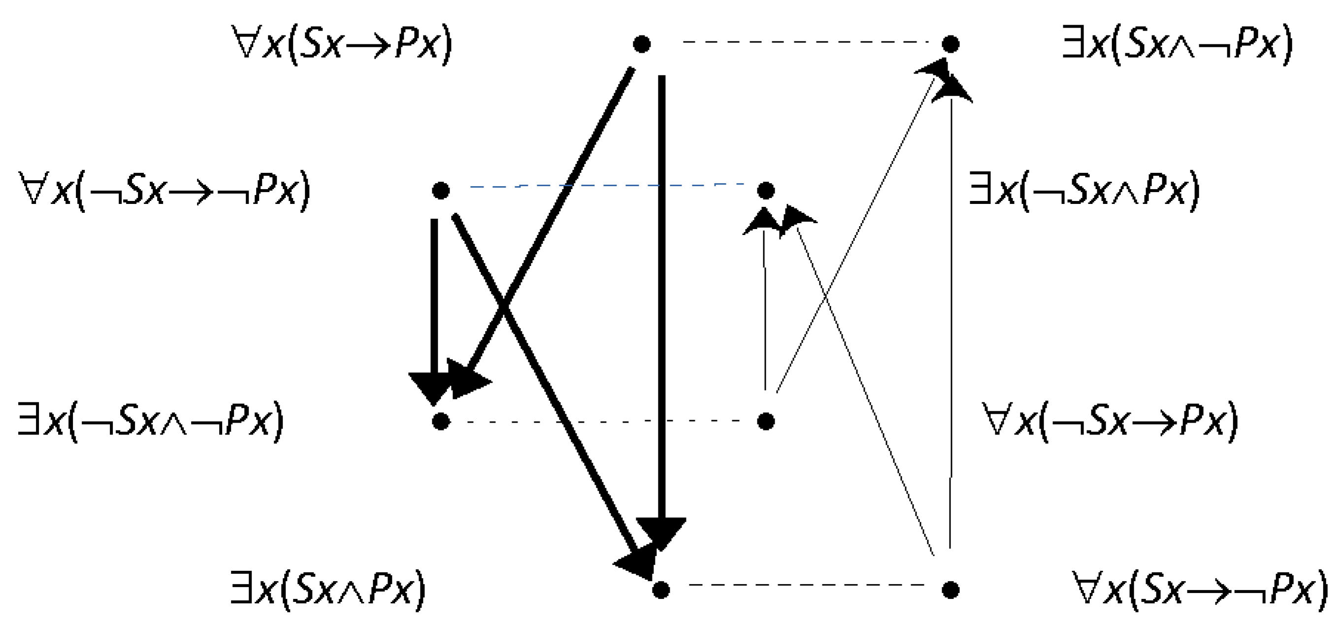
(2) One can partition the set of nodes into two cells, such that (a) every node in a cell has a contradictory in the other cell and (b) no subaltern of a node in a cell is in the other cell.

Clearly, (2a) implies condition (1). In Figure 2, if we take account of the left/right presentation on the page and the syntax of the labels, we can say that the positive nodes are in the left cell while the negative ones are in the right one. Conceptually, there is concord within each cell, opposition between cells.

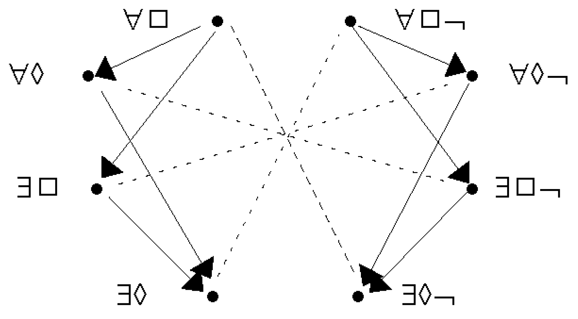
Thanks to property (2), we can twist the right cell, say, like a layer in a Rubik cube so that node ∃◊¬ goes to the top and ∀□¬ to the bottom, the intermediate nodes exchanging positions and all four nodes dragging the ends of the lines that meet them. The lines for the contradictories cease to be diameters and instead become parallel to each other. The subalternation arrows in the right cell now point upwards, while those in the left cell continue to point downwards. One can also smooth away the hour-glasses in Figure 2 without appealing to special conditions by merely nudging node ∃□ to the right and ∃□¬ to the left to create overlapping diamonds. These manipulations are delivered in Figure 3.

The structure of Figure 3 is not new either. It was first used by Lenzen [12], with different labels, in the course of his study of Ploucquet’s work on the quantification of the predicate in the eighteenth century. More recently, it has been used by Makinson [10] in his account of Hamilton’s work on the same topic in the nineteenth century. Diagram 3 of Lenzen [12], intended as a first approximation to Ploucquet’s intentions, is exactly the same as Figure 3, but with other labels in Ploucquet’s long-forgotten notation, which Lenzen transcribes into the language of classical second-order logic. However, on Lenzen’s reading of the eighteenth-century text, Ploucquet’s intended array is not closed under contradictories and so, Lenzen concludes, cannot be diagrammed exactly by Figure 3. To obtain closure under the contradictories, Lenzen enlarged the octagon to a decagon, for which his Diagram 4 again puts contradictories in parallel and reverses appropriate subalternation arrows. Figure 2a of Makinson [10] also has the same structure as Figure 3, with different labels; it approximates the account of quantification of the predicate that was given by Sir William Hamilton in the nineteenth century which, again, was not closed under contradictories.

In the present author’s opinion, the structure of Figure 3 can be taken in at a glance. Moreover, it has the attraction that it can be seen as a two-dimensional representation of a cube, with, say, the left diamond (positive nodes) in the foreground and the right one (negative nodes) in the background. To emphasise that perspective, we have thickened the downward arrows. The four dotted lines for contradictories are parallel edges connecting the front and back faces of the cube.

Given these features, one could describe the contrast between Figure 1 and Figure 3 in any one of several ways, according to the aspect one wishes to emphasise: diametric vs. parallel lines for contradictories, down-only vs. down-and-up arrows for subalternation, or a two-dimensional vs. three-dimensional gestalt for the whole. All three contrasts are present.

The omitted lines for contraries and subcontraries can be recuperated from Figure 3 at will by combining an arrow (or the transitive product of two arrows) with a dotted line using the recipe verified above. Specifically, to find the contraries of a node in the front diamond, one follows arrows down from it and then dotted lines to the rear; for example, the ∀□ node has three contraries ∃□¬, ∀◊¬, ∀□¬, while ∀◊ has as contrary only the last of those, and ∃◊ has none. To find the subcontraries of a node in the front diamond, one retraces arrows up from it and then dotted lines to the rear. Starting instead from the rear diamond, one proceeds dually: for the contraries of a node, one follows arrows up and then to the front, and for the subcontraries, one retraces arrows down and then to the front.

3. Do Not Eliminate all Redundancy!

Although Figure 3 (like Figure 2) gets rid of much of the redundancy in Figure 1, some remains (thanks to Alex Citkin for drawing the author’s attention to this point). If we take as given the subalternations in the left cell, say, together with all the relations of contradiction, we can derive the subalternations of the right cell. For example, the arrow from node ∃□¬ to ∃◊¬ in Figure 3 may be obtained by going round three sides of the top-left face of the cube. Suppose proposition ∃□¬ is true. Then, by the dotted line ∀◊ is false so, retracing the arrow, ∀□ is false so, by its dotted line, ∃◊¬ is true, while if ∃□¬ is false, by the dotted line ∀◊ is true, but by the direction of the arrow, ∀□ may still be false, so ∃◊¬ may still be true. Note that in this verification, we are again using only relations hypothesised between nodes and not the internal logic of the labels on the nodes; the argument still stands when the nodes have other labels.

If we strip out these redundancies as well, we get Figure 4 and, theoretically, one could work with it without a loss of content. But it lacks another desideratum for a good diagram: ease of recuperation of its implicit information. While Figure 1 displayed too much for immediate visual absorption, Figure 4 provides too little for rapid mental calculation of the omitted items. The implicit information can be dug out, but the operations involved go beyond comfortable execution without pencil and paper. In the author’s view, Figure 3 provides the best compromise between exhibiting too much and displaying too little.

4. A Simpler Version of Condition (2)

Given the satisfaction of condition (1) along with the background condition of parsimony, condition (2) is equivalent to the following simpler requirement:

(2′) One can partition the set of nodes into two cells such that within each cell, every pair is consistent.

From a traditional perspective, this requirement is quite natural, reflecting the idea of peace within each cell. Roughly speaking, it tells us that we have positives and negatives, and all oppositions arise between the two categories rather than within them.

Verification. Consider any partition of the node set into two cells. Suppose that it fails condition (2); we show that it fails (2′). By the supposition, there are nodes m, n such that either (a) n is the contradictory of m and they are in the same cell, or (b) n is a subaltern of m and they are in different cells. In case (a), the nodes m, n form an inconsistent pair from the same cell. In case (b), consider the contradictory c(n) of n. If it is in the same cell as n, then n, c(n) forms an inconsistent pair from the same cell. If it is not in the same cell as n, then it is in the same cell as m. But if m is true then its subaltern n must be true, so c(n) must be false; so m, c(n) form an inconsistent pair from the same cell. Thus, in all cases, condition (2′) fails.

Conversely, suppose that the partition fails condition (2′), we show that it fails (2). By the supposition, there is an inconsistent pair of nodes m, n in the same cell. If c(n) is in the same cell as n, then condition (2a) fails for the partition. Suppose on the other hand that c(n) is not in the same cell as n. Since c(n) is the contradictory of a node inconsistent with m, we know that m logically implies c(n), so c(n) must be either a subaltern of m or equivalent to m. But since m, c(n) are in different cells, they are distinct nodes, so the latter case is impossible by the background condition of parsimony (see Section 2; this is the only point in the paper where parsimony is indispensable). And in the former case, a subaltern c(n) of m is in a different cell than m, contrary to condition (2b). Thus, in both cases, condition (2) fails.

The equivalence of conditions (2) and (2′) given condition 1 justifies a minimal kit for constructing polygons of opposition with 2n nodes satisfying conditions (1) and (2). Take any set of n ≥ 2 non-equivalent propositions that are pairwise-consistent and such that their negations are also pairwise-consistent. Then, the given propositions and their negations form a collection of 2n propositions that are clearly non-equivalent, satisfy condition (1), and also satisfy condition (2′) with the given propositions as forming one cell and their negations the other. Hence, as just shown, they also satisfy condition (2).

We may thus draw a polygon of opposition for these 2n propositions, as a three-dimensional figure with a front face and a back face. The front face has nodes for the n given propositions and arrows for whatever subaltern relations hold between them. The back face has nodes for their n contradictories, with the lines linking contradictories running in parallel between front and back faces, just as in Figure 3. The subalternation arrows on the back face reverse those of their contradictories on the front face.

Evidently, in the case n = 4, this construction gives us an octagon; when, in addition, the propositions form a diamond under subalternation, then we get the specific configuration represented by Figure 3.

In the limiting case that n = 2, we get a square of opposition. However, that square is unlike the familiar one, since the two lines for contradictories run left–right in parallel, and the arrow for subalternation on the right points upwards. It thus corresponds to any one of the four side faces of Figure 3. Interestingly, it is the figure that Christensen [2] contends may have been in Aristotle’s mind when writing about oppositions in the Prior Analytics 51b. It is also the preferred display pattern for the square of opposition in Lenzen [12] (p. 45).

5. Limits to the Manipulations

We look at two kinds of limitation: those where condition (1) or (2) fails, and those where both conditions hold but the manipulations that they support do little to enhance the value of the diagram.

As mentioned in Section 2, there is a small percentage of examples in the medieval and later literature for which condition (1) fails, thus risking loss of information when pruning lines for contraries and subcontraries. For example, as mentioned in note 8, if one takes either Ploucquet’s or Hamilton’s account of quantification of the predicate à la lettre, without enlargement or modification, the output array fails that condition.

The present author has not come across any traditional examples of octagons of opposition in which condition (1) is satisfied but (2) fails, and Lorenz Demey has kindly indicated (in an email of 21 January 2024) that he has not noticed any in the ‘Leonardi’ database, at least from among those dating from before 1850. On reflection, this situation is not surprising since, as just shown, all we need to obtain (2) when we have (1) is the simple and natural condition (2′).

Nevertheless, from a modern perspective, examples satisfying (1) but failing (2′), and hence also failing (2), are easy to find.

One kind of example arises when a node m is inconsistent. For then m is inconsistent with itself, so that the cell containing it contains an inconsistent pair (m,m), failing (2′). Another kind of example arises when there are at least three distinct nodes, k, m, n, each of which is inconsistent with each of the other two. If k, m are in the same cell then that cell contains an inconsistent pair, violating (2′), while if they are in different cells then n must be in the same cell as one of them, again contravening (2′).

On the algebraic level, the first kind of example already implies that no subset of the nodes can form a Boolean algebra without violating (2′), for such algebras contain a zero element. The second kind of example tells us a bit more: no subset of the nodes can form what is left of a Boolean algebra of more than four elements when we discard its unit and zero elements. For, by the representation theorem for Boolean algebras, such an algebra is isomorphic to the field of all subsets of a set K containing at least three distinct elements a, b, c. Consider the three singleton subsets {a}, {b}, {c} of K and note that each pair has an empty intersection.

These examples bring out a deep difference between traditional and later perspectives for studying logical relations between propositions. The square of opposition, as well as its generalisation to polygons satisfying condition (2), encourages a vision of propositions as being of two kinds: affirmative and negative. Items of each kind are seen as consistent with others of the same kind; inconsistency is confined to relations between those of opposite kinds. But from a Boolean standpoint, the distinction between affirmatives and negatives is syntax-dependent and not always well defined; inconsistency holds between some propositions of the same as well as of opposite kinds; and, in general, the dichotomy is a poor guide to logical analysis, especially when it is made in terms of a natural language rather than a formal one.

We turn now to some configurations that satisfy condition (2), and thus also condition (1), but where diagrammatic transformations that the condition justifies, similar to those that took us from Figure 1, Figure 2 and Figure 3, do little to improve visual effect.

Consider the ‘Keynes–Johnson octagon’ in Figure 2 of Demey and Smessaert [13], which represents the four traditional categoricals accompanied by another four with negated subjects, read under the background assumption that terms are neither empty nor universal. In this case, conditions (1) and (2) are both satisfied (for a suitable choice of partition), so our operations may be affected. The output may be seen as an angular hour-glass lying on its side, as in Figure 5, where the bold arrows on the left indicate the front face. But while this is a three-dimensional object, it lacks the familiarity of the cube in Figure 3 and has rather less visual impact.

For a more extreme example, constructed from a ‘propositional’ rather than ‘categorical’ perspective, consider an octagon whose nodes, placed on the circumference of a circle, are labelled by four propositional variables p, q, r, s and their negations ¬p, ¬q, ¬r, ¬s, with the four contradictories linked by diameters. Partition these eight formulae into two cells, the positives and the negatives. Evidently, the octagon is parsimonious, and it is closed under contradictories so that condition (1) is satisfied. So is condition (2): contradictories are never in the same cell, and since there are no subalternations between nodes, no subaltern of a node in one cell is in the other cell. In terms of condition (2′), satisfaction is even more obvious since each cell is consistent and thus pairwise-consistent.

Thus, in this example, our diagrammatic manipulations may be carried out. But, since there are no contrary or subcontrary relations between nodes, the pruning operation changes nothing. We may twist the negative cell, say, to obtain the lines for contradictories parallel to each other, but without any three-dimensional effect or other visual advantage.

Another example, where each cell is inconsistent although its elements are pairwise-consistent, is made up of p↔q, q↔r, r↔s, s↔¬p and their negations.

6. General Conclusions

For Aristotelian octagons of opposition satisfying the broad conditions (1), (2), we have not just one but at least two useful kinds of display, exemplified by Figure 1 and Figure 3 above. Choice between displays depends on many factors: what one’s primary goals are when drawing the diagram (e.g., logical insight vs. aesthetic appeal), to whom the diagram is directed (e.g., a broad readership vs. a narrow circle of professionals), and what technical devices are available (e.g., colours and realistic 3D effects). But for communicating a logical structure to a broad range of readers via the printed page or on screens with just basic software, the display in Figure 3 appears to be more effective. Moreover, nothing stops one from satisfying competing virtues by providing more than one diagram for the same configuration. Indeed, in the author’s view, that may be the best practice.

References

- Kneale, W.; Kneale, M. The Development of Logic; Clarendon Press: Oxford, UK, 1962. [Google Scholar]
- Christensen, R. The first square of opposition. Phronesis 2023, 68, 371–383. [Google Scholar] [CrossRef]
- Demey, L.; Smessaert, H. The relationship between Aristotelian and Hasse diagrams. In Diagrams 2014; (LNAI 8578); Dwyer, T., Purchase, H., Delaney, A., Eds.; Springer Nature: Cham, Switzerland, 2014; pp. 213–227. [Google Scholar]
- Demey, L. Boolean considerations on John Buridan’s octagons of opposition. Hist. Philos. Log. 2019, 40, 116–134. [Google Scholar] [CrossRef]
- Klima, G. John Buridan, Summulae de Dialectica; Yale University Press: New Haven, CO, USA, 2001. [Google Scholar]
- De Celaya, J. Commentary on Petrus Hispanus. 1525. Available online: https://gallica.bnf.fr/ark:/12148/bpt6k109374h/f140.item (accessed on 15 January 2024).
- McNamara, P. Making room for going beyond the call. Mind 1996, 105, 415–450. [Google Scholar] [CrossRef]
- Seuren, P.A.M. The cognitive ontogenesis of predicate logic. Notre Dame J. Form. Log. 2014, 55, 499–532. [Google Scholar] [CrossRef]
- Demey, L.; Smessaert, H. A database of Aristotelian diagrams: Empirical foundations for logical geometry. In Diagrams 2022; (LNAI 13462); Giardino, V., Linker, S., Burns, R., Belluci, F., Boucheix, J.-M., Viana, P., Eds.; Springer Nature: Cham, Switzerland, 2022; pp. 123–131. [Google Scholar]
- Makinson, D. Hamilton’s Cumulative Conception of Quantifying Particles: An Exercise in Third-Order Logic (Extended Text). Available online: https://sites.google.com/site/davidcmakinson/ (accessed on 10 April 2024).
- Johnson, W.E. Logic; Cambridge University Press: Cambridge, UK, 1921; Volume I. [Google Scholar]
- Lenzen, W. Ploucquet’s ‘refutation’ of the traditional square of opposition. Log. Universalis 2008, 2, 43–58. [Google Scholar] [CrossRef]
- Demey, L.; Smessaert, H. Aristotelian and Boolean Properties of the Keynes-Johnson Octagon of Opposition. To appear.
Figure 1.
Buridan’s modal octagon, as presented by Demey [4] (p. 120).
Figure 2.
Buridan’s modal octagon pruned.
Figure 3.
Buridan’s modal octagon pruned with a partitioned twist.
Figure 4.
Buridan’s modal octagon with all redundancies eliminated.
Figure 5.
Keynes–Johnson octagon pruned with partitioned reversal.
Disclaimer/Publisher’s Note: The statements, opinions and data contained in all publications are solely those of the individual author(s) and contributor(s) and not of MDPI and/or the editor(s). MDPI and/or the editor(s) disclaim responsibility for any injury to people or property resulting from any ideas, methods, instructions or products referred to in the content. |
© 2024 by the author. Licensee MDPI, Basel, Switzerland. This article is an open access article distributed under the terms and conditions of the Creative Commons Attribution (CC BY) license (https://creativecommons.org/licenses/by/4.0/).
Share and Cite
MDPI and ACS Style
Makinson, D. Display Conventions for Octagons of Opposition. Axioms 2024, 13, 287. https://doi.org/10.3390/axioms13050287
AMA Style
Makinson D. Display Conventions for Octagons of Opposition. Axioms. 2024; 13(5):287. https://doi.org/10.3390/axioms13050287
Chicago/Turabian StyleMakinson, David. 2024. "Display Conventions for Octagons of Opposition" Axioms 13, no. 5: 287. https://doi.org/10.3390/axioms13050287
Note that from the first issue of 2016, this journal uses article numbers instead of page numbers. See further details here.