Sparse Signal Recovery via Rescaled Matching Pursuit

Abstract

We propose the Rescaled Matching Pursuit (RMP) algorithm to recover sparse signals in high-dimensional Euclidean spaces. The RMP algorithm has less computational complexity than other greedy-type algorithms, such as Orthogonal Matching Pursuit (OMP). We show that if the restricted isometry property is satisfied, then the upper bound of the error between the original signal and its approximation can be derived. Furthermore, we prove that the RMP algorithm can find the correct support of sparse signals from random measurements with a high probability. Our numerical experiments also verify this conclusion and show that RMP is stable with the noise. So, the RMP algorithm is a suitable method for recovering sparse signals.

1. Introduction

Compressed sensing (or compressive sensing) [1] has become a very active research direction in the field of signal processing, after the pioneering work by Candès and Tao (see [2]). It has been successfully applied in image compression, signal processing, medical imaging, and computer science (see [3,4,5,6,7]). Compressed sensing refers to the problem of recovering sparse signals from low dimensional measurements (see [8]). In terms of image processing, one needs to compress the image first, then the image signal becomes sparse and its reconstruction belongs to the category of compressed sensing.

Let ${\mathbb{R}}^d$ denote the d-dimensional Euclidean space. Consider a signal $x\in {\mathbb{R}}^d$. We say x is a k-sparse vector if $\#\mathrm{supp}\left(x\right)⩽k$. Here, we use $\mathrm{supp}\left(x\right)$ to denote the set of index such that $x_i\ne 0$ for all $i\in \mathrm{supp}\left(x\right)$ and $\#A$ represents the cardinality of a set A. By the compressed sensing theory, the recovery of a sparse signal can be mathematically described as

$$\begin{array}{c}\hfill f=\Phi x\end{array}$$

(1)

where x is a d-dimensional k-sparse vector, and $\Phi \in {\mathbb{R}}^{N\times d}$ is the measurement matrix with $N\ll d$. The goal of signal recovery is establishing an algorithm to approximate the unknown signal x by using the measurement matrix $\Phi$ and given data $f=\Phi x$.

A well-known method in compressed sensing is basis pursuit (BP), which is also known as ${\ell }_1$ minimization (see [9]). It is defined as

$$\begin{array}{c}\hfill \widehat{x}=arg\underset{x\in {\mathbb{R}}^d}{min}{\{\parallel x\parallel }_{{\ell }_1}:\mathrm{subject}\mathrm{to}f=\Phi x\}\end{array}$$

(2)

By imposing a “restricted orthonormality hypothesis”, which is far weaker than assuming orthonormality and defined as the following Definition 1, the ${\ell }_1$ minimization program can recover x exactly. Furthermore, the target sparse signal x could be recovered with a high probability when $\Phi$ is a Gaussian random matrix.

Definition 1.

A matrix Φ is said to satisfy the restricted isometry property at sparsity level k with the constant ${\delta }_k\in (0,1)$ if

$$\begin{array}{c}\hfill (1-{\delta }_k){\parallel x\parallel }_2^2⩽{\parallel \Phi x\parallel }_2^2⩽(1+{\delta }_k){\parallel x\parallel }_2^2\end{array}$$

holds for all k-sparse vectors x. And, we say that the matrix Φ satisfies the restricted isometry property with parameters $(k,\delta )$ if ${\delta }_k<\delta$.

The ${\ell }_1$ minimization method and related algorithms found by solving (2) have been well studied, and they range widely in effectiveness and complexity (see [1,2,10,11,12]). It is known that a linear program problem can be solved in polynomial time by using optimization software. However, it still takes a long time if the length of the signal is large.

Compared with the BP algorithm, greedy-type algorithms are easy to implement and have less computational complexity and fast convergence speed. Thus, greedy-type algorithms are powerful methods for the recovery of signals and are increasingly used in that field; for example, see [13,14,15,16,17]. To recall this type of algorithm, we first recall some basic notions on sparse approximation in a Hilbert space H. We denote the inner product of H by $〈·,·〉$. The norm $\parallel ·\parallel$ on H is defined by $\parallel f\parallel ={〈f,f〉}^{1/2}$ for all $f\in H$. We call a set $\mathcal{D}\subset H$ a dictionary if the closure of $\mathrm{span}\left(\mathcal{D}\right)$ is H. Here $\mathrm{span}\left(\mathcal{D}\right)$ is the linear space spanned by $\mathcal{D}$. We only consider normalized dictionaries, that is, for any $\phi \in \mathcal{D}$, $\parallel \phi \parallel =1$. Let ${\Sigma }_m\left(\mathcal{D}\right)$ denote the set of all elements which can be expressed as a linear combination of m elements from $\mathcal{D}$

$$\begin{array}{c}\hfill {\Sigma }_m\left(\mathcal{D}\right):=\left\{g:g=\sum _{\phi \in \Lambda }{c}_{\phi }\phi ,\phi \in \mathcal{D},\#\Lambda ⩽m\right\}\end{array}$$

We define the minimal error of the approximation of an element $f\in H$ as $g\in {\Sigma }_m\left(\mathcal{D}\right)$

$$\begin{array}{c}\hfill {\sigma }_m\left(f\right):={\sigma }_m(f,\mathcal{D})=\underset{g\in {\Sigma }_m\left(\mathcal{D}\right)}{inf}\parallel f-g\parallel \end{array}$$

Let a dictionary $\mathcal{D}$ be given. We define the collection of elements by

$$\begin{array}{c}\hfill {\mathcal{A}}_1^o(\mathcal{D},M):=\left\{f\in H:f=\sum _{k\in \Lambda }{c}_k\left(f\right){\phi }_k,{\phi }_k\in \mathcal{D},\#\Lambda ⩽\infty ,\sum _{k\in \Lambda }\left|c_k\left(f\right)\right|⩽M\right\}\end{array}$$

Then, we define ${\mathcal{A}}_1(\mathcal{D},M)$ to be the closure of ${\mathcal{A}}_1^o(\mathcal{D},M)$ in H. Finally, we define the linear space ${\mathcal{A}}_1\left(\mathcal{D}\right)$ by

$${\mathcal{A}}_1\left(\mathcal{D}\right):=\bigcup _{M>0}{\mathcal{A}}_1(\mathcal{D},M)$$

and we equip ${\mathcal{A}}_1\left(\mathcal{D}\right)$ with the norm

$$\begin{array}{c}\hfill {\parallel f\parallel }_{{\mathcal{A}}_1\left(\mathcal{D}\right)}:=inf\{M:f\in {\mathcal{A}}_1(\mathcal{D},M)\}\end{array}$$

for all $f\in {\mathcal{A}}_1\left(\mathcal{D}\right)$.

The simplest greedy algorithm in H is known as the Pure Greedy Algorithm (PGA$(H,\mathcal{D})$). We recall its definition from [18].

Pure Greedy Algorithm (PGA($\mathit{H}$, $\mathcal{D}$))

Step 1: Set $f_0=0$.

Step 2:

-If $f=f_{m-1}$, then stop and define $f_l=f_{m-1}=f$ for $l\ge m$.

-If $f\ne f_{m-1}$, then choose an element ${\phi }_m\in \mathcal{D}$ satisfying

$$|\langle f-f_{m-1}^{PGA},{\phi }_m\rangle |=\underset{\phi \in \mathcal{D}}{sup}\left|\langle f-f_{m-1}^{PGA},\phi \rangle \right|$$

Define the new approximation of f as

$$f_m^{PGA}=\sum _{i=1}^m\langle f-f_{m-1}^{PGA},{\phi }_i\rangle {\phi }_i$$

and proceed to Step 2.

In [19], DeVore and Temlyakov proposed the Orthogonal Greedy Algorithm (OGA$(H,\mathcal{D})$) in H with a dictionary $\mathcal{D}$. We recall its definition.

Orthogonal Greedy Algorithm (OGA($\mathit{H}$, $\mathcal{D}$))

Step 1: Set $f_0=0$.

Step 2:

-If $f=f_{m-1}$, then stop and define $f_l=f_{m-1}=f$ for $l⩾m$.

-If $f\ne f_{m-1}$, then choose an element ${\phi }_m\in \mathcal{D}$ satisfying

$$|\langle f-f_{m-1}^{OGA},{\phi }_m\rangle |=\underset{\phi \in \mathcal{D}}{sup}\left|\langle f-f_{m-1}^{OGA},\phi \rangle \right|$$

Define the new approximation of f as

$$f_m^{OGA}=P_m\left(f\right)$$

where $P_m\left(f\right)$ is the best approximation of f from the linear space $V_m$ := span$\{{\phi }_1,{\phi }_2,···,{\phi }_m\}$, and proceed to Step 2.

In fact, the OGA is one of the modifications of the PGA, improving the convergence rate. The convergence rate is one of the critical issues for the approximation power of algorithms. If $f_m$ is the approximation of the target element f by applying a greedy algorithm after m iterations, the efficiency of the algorithm can be measured by the decay of the sequence $\{\parallel f-f_m\parallel \}$. It has been shown that the PGA and the OGA can achieve the convergence rates $m^{-1/6}$ and $m^{-1/2}$ for $\parallel f-f_m\parallel$, respectively, if the target element f belongs to ${\mathcal{A}}_1(\mathcal{D},M)$ (see [19]).

Theorem 1.

Suppose $\mathcal{D}$ is a dictionary of H. Then, for every $f\in {\mathcal{A}}_1(\mathcal{D},M),$ the following inequality holds:

$$\parallel f-f_m^{PGA}\parallel \le M{m}^{-1/6},m=0,1,2,\cdots .$$

Theorem 2.

Suppose $\mathcal{D}$ is a dictionary of H. Then, for every $f\in {\mathcal{A}}_1(\mathcal{D},M),$ the following inequality holds:

$$\parallel f-f_m^{OGA}\parallel \le M{m}^{-1/2},m=0,1,2,\cdots .$$

It is known from [20] that the convergence rate $m^{-1/2}$ cannot be improved. Thus, as a very general result for all dictionaries, the convergence rate is optimal.

The fundamental problem of signal recovery is to find out the support of the original target signal by using the model (1). Since N is much smaller than the dimension d, the column vectors of the measurement matrix $\Phi$ are linearly dependent. Therefore, these vectors consist of a redundant system. This redundant system may be considered as a dictionary of ${\mathbb{R}}^N$. It is well known that ${\mathbb{R}}^N$ is a Hilbert space with the usual inner product

$$\begin{array}{c}\hfill 〈x,y〉=\sum _{j=1}^N{x}_j{y}_j,\forall x\in {\mathbb{R}}^N,y\in {\mathbb{R}}^N\end{array}$$

Thus, signal recovery can be considered as an approximation problem with a dictionary in a Hilbert space. In particular, the approximation of the original signal is the solution of the following minimization problem:

$$\begin{array}{c}\hfill \underset{{\widehat{x}}_1,\cdots ,{\widehat{x}}_d\in \mathbb{R}}{min}\parallel f-\sum _{i=1}^d{\widehat{x}}_i{\phi }_i{\parallel }_2\end{array}$$

where ${\phi }_1,\cdots ,{\phi }_d$ denote the columns of $\Phi$. Naturally, one can adapt greedy approximation algorithms to handle the signal recovery problem. In CS, one such method is Orthogonal Matching Pursuit (OMP) (see [21,22]), which is an application of OGA to the field of signal processing. Compared with the BP, the OMP is faster and it admits an ease of implementation (see [17,23]). We recall the definition of the OMP from [23].

Orthogonal Matching Pursuit (OMP)

Input: An $N\times d$ matrix $\Phi$, $f\in {\mathbb{R}}^N$, the sparsity index k.

Step 1: Set $r_0=f$, the index set ${\Lambda }_0=\varnothing$, and $m=1$.

Step 2: Define ${\Lambda }_m:={\Lambda }_{m-1}\cup \left\{i_m\right\}$ such that

$$\begin{array}{c}\hfill |〈r_{m-1},{\phi }_{i_m}〉|=\underset{\phi \in \Phi }{sup}\left|〈r_{m-1},\phi 〉\right|\end{array}$$

Then,

$$\begin{array}{c}\hfill x_m=\underset{z:\mathrm{supp}\left(z\right)\in {\Lambda }_m}{argmin}{\parallel f-\Phi z\parallel }_2,f_m^o=\Phi x_m\end{array}$$

and

$$\begin{array}{c}\hfill r_m=f-f_m^o=f-\Phi x_m\end{array}$$

Step 3: Increment m, and return to Step 2 if $\#{\Lambda }_m<k$.

Output: If $\#{\Lambda }_m⩾k$, then output ${\Lambda }_m$ and $\widehat{x}=x_m$.

It is clear from the available literature that the OMP algorithm is the most popular greedy-type algorithm being used for signal recovery. The OMP algorithm, with a high probability, can exactly recover each sparse signal by using a Gaussian or Bernoulli matrix (see [17]). And, it is shown that the OMP algorithm can stably recover sparse signals in $l^2$ under measurement noise (see [24]). Although the OMP algorithm is powerful, the computational complexity of the orthogonality step is quite high, especially for large-scale problems. See [25] for the detailed computation and the storage cost of the OMP. So, the main disadvantage of the OMP is its high computational cost. In particular, when the sparsity level k of the target signal is large, OMP may not be a good choice, since the cost of orthogonalization increases quadratically with the number of iterations. Thus, in this case, it is natural to look for other greedy-type algorithms to reduce the computational cost.

In Section 2, we propose an algorithm called Rescaled Matching Pursuit (RMP) for signal recovery. This algorithm has less computational complexity than the OMP, which means it can save resources such as storage space and computation time. In Section 3, we analyze the efficiency of the RMP algorithm under the RIP condition. In Section 4, we prove that the RMP algorithm can be used to find the correct support of sparse signal from a random measurement matrix with a high probability. In Section 5, we use numerical experiments to verify this conclusion. In Section 6, we summarize our results.

2. Rescaled Matching Pursuit Algorithm

In [26], Petrova presented another modification of the PGA which is called the escaled pure greedy algorithm (RPGA). This modification is very simple. It simply rescales the approximation in each iteration of the PGA.

We recall the definition of the RPGA(H, $\mathcal{D})$ from [26].

Rescaled Pure Greedy Algorithm (RPGA($\mathit{H}$, $\mathcal{D}$))

Step 1: Set $f_0=0,r_0=f$.

Step 2:

-If $f=f_{m-1}$, then stop and define $f_k=f_{m-1}=f$ for $k\ge m$.

-If $f\ne f_{m-1}$, then choose an element ${\phi }_m\in \mathcal{D}$ satisfying

$$|\langle r_{m-1},{\phi }_m\rangle |=\underset{\phi \in \mathcal{D}}{sup}\left|\langle r_{m-1},\phi \rangle \right|$$

with

$${\lambda }_m=\langle r_{m-1},{\phi }_m\rangle ,{\widehat{f}}_m:=f_{m-1}+{\lambda }_m{\phi }_m,s_m=\frac{\langle f,{\widehat{f}}_m\rangle }{\parallel {\widehat{f}}_m{\parallel }^2}$$

Then, define the the new approximation of f as

$$f_m=s_m{\widehat{f}}_m,r_m=f-f_m$$

and proceed to Step 2.

The following theorem on the convergence rate of the RPGA was also obtained in [26].

Theorem 3.

Suppose $\mathcal{D}$ is a dictionary of H. Then, for every $f\in {\mathcal{A}}_1\left(\mathcal{D}\right),$ the RPGA satisfies the following inequality:

$$\parallel f-f_m{\parallel \le \parallel f\parallel }_{{\mathcal{A}}_1\left(\mathcal{D}\right)}{(m+1)}^{-1/2},m=0,1,2,\cdots$$

Notice that the RPGA only needs to solve a one-dimensional optimization problem at each step. Thus, the RPGA is simpler than the OGA. Together with Theorem 3, it is known that the RPGA is a greedy algorithm with minimal computational complexity to achieve the optimal convergence rate $m^{-1/2}$. Based on this result, the RPGA has been applied successfully to solve the problems of convex optimization and regression, see [27,28,29]. In solving these two types of problems, the RPGA performs better than the OGA. The main reason is that the RPGA has smaller computational cost than the OGA. For more detailed results about the RPGA, one can refer to [26,27,28,29,30]. Besides, in [31] the authors propose the Super Rescaled Pure Greedy Learning Algorithm and investigate its behavior. The success of the RPGA inspires us to consider its application in the field of signal recovery.

In the present article, we will design an algorithm based on the RPGA to recover sparse signals and analyze its performance. Suppose that x is a k-sparse signal in ${\mathbb{R}}^d$ and $\Phi$ is an $N\times d$ matrix. We denote the columns of $\Phi$ as ${\phi }_1,\cdots ,{\phi }_d$. Then, we design the Rescaled Matching Pursuit (RMP) for sparse signal recovery.

Rescaled Matching Pursuit (RMP)

Input: Measurement matrix $\Phi$, vector f, the sparsity index k.

Step 1: Set $r_0=f$, $f_0=0$, the index set ${\Lambda }_0=\varnothing$, and $m=1$.

Step 2: Define ${\Lambda }_m:={\Lambda }_{m-1}\cup \left\{i_m\right\}$ such that

$$\begin{array}{c}\hfill |〈r_{m-1},{\phi }_{i_m}〉|=\underset{\phi \in \Phi }{sup}\left|〈r_{m-1},\phi 〉\right|\end{array}$$

Then,

$$f_m=s_m{\widehat{f}}_m$$

where ${\theta }_m=〈r_{m-1},{\phi }_{i_m}〉$, ${\widehat{f}}_m=f_{m-1}+{\theta }_m{\phi }_{i_m}$, and $s_m=\frac{〈f,{\widehat{f}}_m〉}{\parallel {\widehat{f}}_m{\parallel }_2^2}$. Next, update the residual

$$\begin{array}{c}\hfill r_m=f-f_m\end{array}$$

Step 3: Increment m, and return to Step 2 if $\#{\Lambda }_m<k$.

Output: If $\#{\Lambda }_m⩾k$, then output ${\Lambda }_m$ and $\widehat{x}$. It is easy to see that $\widehat{x}$ has nonzero indices at the components listed in ${\Lambda }_m$. If $i_{m_1}=i_{m_2}=\cdots =i_{m_s}=i_j$, then we can figure out the value of $\widehat{x}$ in component $i_j$ through

$$\begin{array}{c}\hfill \widehat{x}\left(i_j\right)=\sum _{l=1}^s{\theta }_{m_l}\prod _{i=m_l}^k{s}_i\end{array}$$

The main procedure of the algorithm can be divided into selecting the columns of $\Phi$ and constructing the approximation $f_m$. In Step 2, the approximation $f_m$ is obtained by solving a one-dimensional optimization problem. In fact, $f_m$ is an orthogonal projection of f onto the one-dimensional space $\mathrm{span}\left\{{\widehat{f}}_m\right\}$. The RMP algorithm is broadly similar to the OMP algorithm, while the computational complexity differs. For the OMP algorithm, the approximation $f_m^o:=\Phi \widehat{x}$ is obtained by solving the m-dimensional least squares problem at m iteration in Step 2, which has a total cost of $O\left(mN\right)$. For the RMP algorithm, as argued above, the approximation $f_m$ is obtained by solving a one-dimensional optimization problem at the m iteration in Step 2, which has a total cost of $O\left(N\right)$. It is not difficult to see that the computational cost is less expensive than most existing greedy algorithms, such as the OMP algorithm. That is, we can save a lot of resources such as storage space and computation time by using the RMP algorithm.

3. Efficiency of the RMP under the Restricted Isometry Property

Suppose that the matrix $\Phi$ satisfies the RIP condition which is defined in Definition 1. Then, we study the performance of the RMP for k-sparse signal recovery.

Under the RIP, we obtain the convergence rate of the error between the given data vector f and its approximation $f_m$.

Theorem 4.

Assume that x is an arbitrary k-sparse signal in ${\mathbb{R}}^d$ and the measurement matrix $\Phi \in {\mathbb{R}}^{N\times d}$ satisfies the RIP condition with parameters $(k,\delta )$. Then, for $f=\Phi x$ and every positive integer m, we have

$$\parallel f-f_m{\parallel }_2⩽\frac{k^{1/2}{\parallel f\parallel }_2}{(1-\delta )}{(m+1)}^{-1/2},m=0,1,\cdots$$

Moreover, we derive the upper bound of the difference between the original signal x and the estimate $\widehat{x}$ of x.

Theorem 5.

Assume that x is an arbitrary k-sparse signal in ${\mathbb{R}}^d$ and the measurement matrix $\Phi \in {\mathbb{R}}^{N\times d}$ satisfies the RIP condition with parameters $(2k,\delta )$. Given the data $f=\Phi x$, if $\#{\Lambda }_L=k,L⩾k$, we have

$$\begin{array}{c}\hfill \parallel x-\widehat{x}{\parallel }_2⩽\frac{k^{1/2}{\parallel f\parallel }_2}{{(1-\delta )}^{3/2}}{(L+1)}^{-1/2}\end{array}$$

To prove Theorems 4 and 5, we will use a lemma which was obtained in [32].

Lemma 1.

Let the positive constants ℓ, r, and B be given. Suppose $\left\{a_m\right\}$ and $\left\{r_m\right\}$ are finite or infinite sequences of positive real numbers such that

$$a_J⩽B,a_m⩽a_{m-1}\left(1-\frac{r_m}{r}{a}_{m-1}^{\ell }\right),m=J+1,J+2,\cdots$$

Then, $a_m$ has the following upper bound:

$$a_m⩽max\{1,{\ell }^{-1/\ell }\}{r}^{1/\ell }{\left(r{B}^{-\ell }+\sum _{k=J+1}^m{r}_k\right)}^{-1/\ell },m=J+1,J+2,\cdots$$

Proof of Theorem 4: 

It follows from the definitions of ${\widehat{f}}_m$ and ${\theta }_m$ that

$$\begin{array}{cc}\hfill \parallel f-{\widehat{f}}_m{\parallel }_2^2& =〈f-{\widehat{f}}_m,f-{\widehat{f}}_m〉\hfill \\ \hfill & =〈f-f_{m-1}-{\theta }_m{\phi }_{i_m},f-f_{m-1}-{\theta }_m{\phi }_{i_m}〉\hfill \\ \hfill & =\parallel f-f_{m-1}{\parallel }_2^2-2{\theta }_m〈f-f_{m-1},{\phi }_{i_m}〉+{\theta }_m^2{\parallel {\phi }_{i_m}\parallel }_2^2\hfill \\ \hfill & =\parallel f-f_{m-1}{\parallel }_2^2-2{〈f-f_{m-1},{\phi }_{i_m}〉}^2+{\parallel {\phi }_{i_m}\parallel }_2^2{〈f-f_{m-1},{\phi }_{i_m}〉}^2\hfill \end{array}$$

From the design of the RMP, we know that $f_m$ is the orthogonal projection of f onto span$\left\{{\widehat{f}}_m\right\}$. Thus, the following must be true:

$$\begin{array}{cc}\hfill \parallel f-f_m{\parallel }_2^2& ⩽\parallel f-{\widehat{f}}_m{\parallel }_2^2\hfill \\ \hfill & =\parallel f-f_{m-1}{\parallel }_2^2-2{〈f-f_{m-1},{\phi }_{i_m}〉}^2+{\parallel {\phi }_{i_m}\parallel }_2^2{〈f-f_{m-1},{\phi }_{i_m}〉}^2\hfill \end{array}$$

We continue to estimate the approximation error of $f_m$ by using the RIP condition with parameters $(k,\delta )$ of the matrix $\Phi$. Hence, the above inequality can be estimated as

$$\begin{array}{cc}\hfill \parallel f-f_m{\parallel }_2^2& ⩽\parallel f-f_{m-1}{\parallel }_2^2-2{〈f-f_{m-1},{\phi }_{i_m}〉}^2+(1+\delta ){〈f-f_{m-1},{\phi }_{i_m}〉}^2\hfill \\ & =\parallel f-f_{m-1}{\parallel }_2^2-(1-\delta ){〈f-f_{m-1},{\phi }_{i_m}〉}^2\hfill \end{array}$$

(3)

Now, we will derive a lower bound for $|〈f-f_{m-1},{\phi }_{i_m}〉|$. Note that $f_m$ is orthogonal to $f-f_m$, that is, the following applies

$$\langle f-f_m,f_m\rangle =0,m\ge 0$$

(4)

It is observed that

$$\begin{array}{c}\hfill f=\Phi x=\sum _{i=1}^d{x}_i{\phi }_i=\sum _{i\in \mathrm{supp}\left(x\right)}{x}_i{\phi }_i\end{array}$$

(5)

From (4), (5), and the Hölder inequality, we have

$$\begin{array}{cc}\hfill \parallel f-f_{m-1}{\parallel }_2^2& =〈f-f_{m-1},f-f_{m-1}〉\hfill \\ \hfill & =〈f-f_{m-1},f〉\hfill \\ \hfill & =\sum _{i\in \mathrm{supp}\left(x\right)}{x}_i〈f-f_{m-1},{\phi }_i〉\hfill \\ \hfill & ⩽\sum _{i\in \mathrm{supp}\left(x\right)}|x_i\left|\right|〈f-f_{m-1},{\phi }_i〉|\hfill \\ \hfill & ⩽|〈f-f_{m-1},{\phi }_{i_m}〉|\sum _{i\in \mathrm{supp}\left(x\right)}\left|x_i\right|\hfill \\ \hfill & ⩽|〈f-f_{m-1},{\phi }_{i_m}〉|k^{1/2}{\left(\sum _{i\in \mathrm{supp}\left(x\right)}{\left|x_i\right|}^2\right)}^{1/2}\hfill \\ \hfill & =k^{1/2}|〈f-f_{m-1},{\phi }_{i_m}〉{|\parallel x\parallel }_2\hfill \end{array}$$

From the RIP condition of $\Phi$ with the parameters $(k,\delta )$, we obtain

$$\begin{array}{cc}\hfill \parallel f-f_{m-1}{\parallel }_2^2& ⩽k^{1/2}|〈f-f_{m-1},{\phi }_{i_m}〉{|\parallel x\parallel }_2\hfill \\ \hfill & ⩽k^{1/2}{(1-\delta )}^{-1/2}|〈f-f_{m-1},{\phi }_{i_m}〉{|\parallel \Phi x\parallel }_2\hfill \\ \hfill & =k^{1/2}{(1-\delta )}^{-1/2}|〈f-f_{m-1},{\phi }_{i_m}〉{|\parallel f\parallel }_2\hfill \end{array}$$

which implies

$$|〈f-f_{m-1},{\phi }_{i_m}〉|⩾\frac{{(1-\delta )}^{1/2}}{k^{1/2}{\parallel f\parallel }_2}{\parallel f-f_{m-1}\parallel }_2^2$$

Thus, combining the above inequality with (3), we have

$$\begin{array}{cc}\hfill \parallel f-f_m{\parallel }_2^2& ⩽\parallel f-f_{m-1}{\parallel }_2^2-(1-\delta )\frac{(1-\delta )}{{k\parallel f\parallel }_2^2}{\parallel f-f_{m-1}\parallel }_2^4\hfill \\ \hfill & =\parallel f-f_{m-1}{\parallel }_2^2\left(1-\frac{{(1-\delta )}^2}{{k\parallel f\parallel }_2^2}{\parallel f-f_{m-1}\parallel }_2^2\right)\hfill \\ \hfill & =\parallel f-f_{m-1}{\parallel }_2^2\left(1-{\left[\frac{k^{1/2}{\parallel f\parallel }_2}{(1-\delta )}\right]}^{-2}{\parallel f-f_{m-1}\parallel }_2^2\right)\hfill \end{array}$$

Note that

$$\begin{array}{c}\hfill \parallel f-f_0{\parallel }^2={\parallel f\parallel }^2⩽\frac{k}{{(1-\delta )}^2}{\parallel f\parallel }_2^2\end{array}$$

Applying Lemma 1 with $a_m={\parallel f-f_m\parallel }_2^2,B={\left(\frac{k^{1/2}{\parallel f\parallel }_2}{1-\delta }\right)}^2,r_m:=1,r={\left(\frac{k^{1/2}{\parallel f\parallel }_2}{1-\delta }\right)}^2,J=0$, and $\ell =1$, then we have

$$\begin{array}{c}\hfill \parallel f-f_m{\parallel }_2^2⩽{\left(\frac{k^{1/2}{\parallel f\parallel }_2}{1-\delta }\right)}^2{(m+1)}^{-1},m⩾1\end{array}$$

which completes the proof of Theorem 4. □

Based on the result of Theorem 4, we can prove Theorem 5.

Proof of Theorem 5: 

If the matrix $\Phi$ satisfies the RIP condition with parameters $(2k,\delta )$, then by Theorem 4, we can estimate the upper bound of $\parallel x-\widehat{x}\parallel$ as follows:

$$\begin{array}{cc}\hfill \parallel x-\widehat{x}{\parallel }_2^2& ⩽{(1-\delta )}^{-1}{\parallel \Phi (x-\widehat{x})\parallel }_2^2\hfill \\ \hfill & ={(1-\delta )}^{-1}{\parallel \Phi x-\Phi \widehat{x}\parallel }_2^2\hfill \\ \hfill & ={(1-\delta )}^{-1}{\parallel f-f_L\parallel }_2^2\hfill \\ \hfill & ⩽\frac{{k\parallel f\parallel }_2^2}{{(1-\delta )}^3}{(L+1)}^{-1}\hfill \end{array}$$

Thus, the proof of Theorem 5 is finished. □

It is known from Theorem 5 that RMP can obtain a good approximation of the sparse signal f. In this case, it is worse than the OMP, since OMP can recover f exactly if the RIP condition is satisfied. The key point is that one can establish the ideal Lebesgue-type inequality for OMP but not for RMP; for example, see [22,33,34]. On the other hand, as far as we know, until now, it is impossible to construct a deterministic matrix satisfying the RIP condition. In practice, one usually uses the random matrix in signal recovery. We will show that the performance of the RMP is similar to the OMP in this case.

4. Signal Recovery with Admissible Measurements

Since one could not construct a deterministic matrix satisfying the RIP condition, it is natural to consider a random matrix. In practice, almost all approaches to recovering sparse signals using greedy-type methods involve some kind of randomness. In this section, we choose a class of random matrices which have good properties. This class of matrices is called admissible matrices. We first recall the definition of this class of matrices. Then, we prove that the support of a k-sparse target signal in ${\mathbb{R}}^d$ can be recovered with a high probability by applying the RMP algorithm. This shows that RMP is a powerful method of recovering sparse signals in high-dimensional Euclidean spaces.

Definition 2.

An admissible measurement matrix for a k-sparse signal in ${\mathbb{R}}^d$ is an $N\times d$ random matrix Φ satisfying the following conditions:

• (M1) The columns of Φ are stochastically independent.
• (M2) $\mathbb{E}(\parallel {\phi }_j{\parallel }_2^2)=1$ for $j=1,\cdots ,d$.
• (M3) Let $\left\{u_m\right\}$ be a sequence of k vectors whose ${\ell }_2$ norm do not exceed 1. If φ is a column of Φ independent from $\left\{u_m\right\}$, then

  $$\begin{array}{c}\hfill Prob\left\{\underset{m}{max}\left|〈\phi ,u_m〉\right|⩽\epsilon \right\}⩾1-2k{e}^{-C_3{\epsilon }^{2}N}\end{array}$$

  for a positive constant $C_3$.
• (M4) For a given $N\times k$ submatrix Z from Φ, the kth largest singular value ${\sigma }_k\left(Z\right)$ satisfies

  $$\begin{array}{c}\hfill \mathrm{Prob}\left\{{\sigma }_k\left(Z\right)⩾\frac{1}{2}\right\}⩾1-e^{-C_{4}N}\end{array}$$

  for a positive constant $C_4$.

We illustrate some points about the conditions (M3) and (M4). The above condition (M3) offers a limitation of the singular value of the submatrix, which is analogous to the RIP condition (see [17]). Furthermore, the condition (M4) controls the inner product, since the selection of index at Step 2 of the RMP algorithm relates to the inner product. Two typical classes of admissible measurement matrices are the Gaussian matrix and Bernoulli matrix, which were first introduced by Candès and Tao for signal recovery and defined as follows (see [2]).

Definition 3.

A measurement matrix Φ is called a Gaussian measurement if every entry of Φ is selected from the Gaussian distribution $\mathcal{N}(0,N^{-1})$, of which the density function $p\left(x\right)$ is$p\left(x\right)=\frac{1}{\sqrt{2\pi N}}{e}^{-x^{2}N/2}$, for $x\in \mathbb{R}$

Definition 4.

A measurement matrix Φ is called a Bernoulli measurement if every entry of Φ is selected to be $\pm \frac{1}{\sqrt{N}}$ with the same probability, i.e., $\mathrm{Prob}\{{\Phi }_{ij}=1/\sqrt{N}\}=\mathrm{Prob}\{{\Phi }_{ij}=-1/\sqrt{N}\}=\frac{1}{2}$, where $i=1,\cdots ,N,j=1,\cdots ,d$.

Obviously, for Gaussian and Bernoulli measurements, the properties (M1) and (M2) are straightforward to verify. We can check the other two properties using the following known results. See [17] for more details.

Proposition 1.

Suppose $\left\{u_m\right\}$ is a sequence of k-sparse vectors. The ${\ell }_2$ norm of each $u_m$ does not exceed 1. Choose z independently to be a random vector with $i.i.d.\mathcal{N}(0,N^{-1})$ entries. Then

$$\begin{array}{c}\hfill \mathrm{Prob}\left\{\underset{m}{max}\left|〈z,u_m〉\right|⩽\epsilon \right\}⩾1-k{e}^{-2{\epsilon }^{2}N/2}\end{array}$$

Proposition 2.

Let Z be an $N\times k$ matrix whose entries are all $i.i.d.\mathcal{N}(0,N^{-1})$ or else $i.i.d.$ uniform on $\pm \frac{1}{\sqrt{N}}$. Then

$$\begin{array}{c}\hfill \frac{1}{2}{\parallel x\parallel }_2⩽{\parallel Z\parallel }_2⩽\frac{3}{2}{\parallel x\parallel }_2,\mathrm{for}\mathrm{all}x\in {\mathbb{R}}^k\end{array}$$

with a probability of at least

$$\begin{array}{c}\hfill 1-2·{24}^k·e^{-cN}\end{array}$$

For the RMP algorithm, we derive the following result.

Theorem 6.

Let x be a k-sparse signal in ${\mathbb{R}}^d$ and Φ be an $N\times d$ admissible matrix independent from the signal. For the given data $f=\Phi x$, if the RMP algorithm selects k elements in the first $L⩾k$ iterations, the correct support of x can be found with the probability exceeding $1-4L(d-k)e^{-cN/k}$, where c is a constant dependent on the admissible measurement matrix Φ.

Proof of Theorem 6: 

Without a loss of generality, we may assume that the first k components of x are nonzero and the other remaining components of x are zeroes. Obviously, f can be expressed as a linear combination of the first k columns of measurement matrix $\Phi$. We decompose the measurement matrix $\Phi$ into two parts $\Phi =\left[{\Phi }_{opt}\right|\Psi ]$, where ${\Phi }_{opt}$ is the submatrix formed by the first k columns of $\Phi$, and $\Psi$ is the submatrix formed by the remaining $d-k$ columns. For ${\Phi }_{opt}$, we assume that

$$\begin{array}{c}\hfill {\Phi }_{opt}=[{\phi }_1,\cdots ,{\phi }_k],{\phi }_1,\cdots ,{\phi }_k\in \Phi \end{array}$$

and

$$\begin{array}{c}\hfill f=\Phi x=\sum _{i=1}^k{\phi }_i{x}_i\end{array}$$

Furthermore, we can know that $f=\Phi x$ is independent from the random matrix $\Psi$.

Denote $E_{succ}$ as the event where the RMP algorithm recovers all k elements from the support of x correctly in the first $L⩾k$ iterations. Define $\Sigma$ as the event where ${\sigma }_k\left({\Phi }_{opt}\right)⩾\frac{1}{2}$. Then, we have

$$\begin{array}{cc}\hfill \mathrm{Prob}\left\{E_{succ}\right\}& ⩾\mathrm{Prob}\{E_{succ}\cap \Sigma \}\hfill \\ \hfill & =\mathrm{Prob}\left\{E_{succ}\right|\Sigma \}·\mathrm{Prob}\{\Sigma \}\hfill \end{array}$$

For an N-dimensional vector r, define

$$\begin{array}{c}\hfill \rho \left(r\right):=\frac{\parallel {\Psi }^T{r\parallel }_{\infty }}{\parallel {\Phi }_{opt}^T{r\parallel }_{\infty }}=\frac{{max}_{\psi }\left|〈\psi ,r〉\right|}{\parallel {\Phi }_{opt}^T{r\parallel }_{\infty }}\end{array}$$

where $\psi$ is a column of the matrix $\Psi$. If r is a residual vector derived by the Step 2 of the RMP algorithm and $\rho \left(r\right)$ satisfies $\rho \left(r\right)<1$, it means that a column from matrix ${\Phi }_{opt}$ has been selected.

If we execute the RMP algorithm with input signal x and measurement matrix ${\Phi }_{opt}$ for L iterations, then we obtain a sequence of residual vectors $r_0,r_1,\cdots ,r_{L-1}$. Obviously, the residual vectors are independent from the matrix $\Psi$ and can be considered as the functions of x and ${\Phi }_{opt}$. Instead, suppose that we execute the RMP algorithm with the input signal x and matrix $\Phi$ for L iterations. If the RMP algorithm recovers all the k elements of the support of x correctly, the columns of ${\Phi }_{opt}$ should be selected at each iteration. Thus, the sequence of residual vectors should be same as when we execute the algorithm with ${\Phi }_{opt}$.

Therefore, the condition probability satisfies

$$\begin{array}{c}\hfill \mathrm{Prob}\left\{E_{succ}\right|\Sigma \}⩾\mathrm{Prob}\{\underset{m}{max}\rho \left(r_m\right)<1|\Sigma \}\end{array}$$

where $r_m$ is a random vector depending on ${\Phi }_{opt}$ and stochastically independent from $\Psi$.

Assume that $\Sigma$ occurs. Since ${\Phi }_{opt}^{T}r$ is a k-dimensional vector, then

$$\begin{array}{c}\hfill \rho \left(r_m\right)=\frac{{max}_{\psi }\left|〈\psi ,r_m〉\right|}{\parallel {\Phi }_{opt}^T{r}_m{\parallel }_{\infty }}⩽\frac{\sqrt{k}{max}_{\psi }\left|〈\psi ,r_m〉\right|}{\parallel {\Phi }_{opt}^T{r}_m{\parallel }_2}\end{array}$$

By the basic property of singular values, we have

$$\begin{array}{c}\hfill \frac{\parallel {\Phi }_{opt}^T{r\parallel }_2}{{\parallel r\parallel }_2}⩾{\sigma }_k\left({\Phi }_{opt}\right)⩾\frac{1}{2}\end{array}$$

for any vector r in the range of ${\Phi }_{opt}$. Thus, for vector $r_m$, we have $\parallel u_m{\parallel }_2⩽1$, where $u_m:=\frac{1}{2}\frac{r_m}{\parallel {\Phi }_{opt}^T{r}_m{\parallel }_2}$. Then, the have the following:

$$\begin{array}{cc}\hfill \rho \left(r_m\right)& ⩽\frac{\sqrt{k}{max}_{\psi }\left|〈\psi ,r_m〉\right|}{\parallel {\Phi }_{opt}^T{r}_m{\parallel }_2}\hfill \\ \hfill & =2\sqrt{k}\underset{\psi }{max}\left|〈\psi ,\frac{r_m}{2\parallel {\Phi }_{opt}^T{r}_m{\parallel }_2}〉\right|\hfill \\ \hfill & =2\sqrt{k}\underset{\psi }{max}\left|〈\psi ,u_m〉\right|\hfill \end{array}$$

for each index $m=0,1,\cdots ,L-1$.

Thus, we have

$$\begin{array}{c}\hfill \mathrm{Prob}\{\rho \left(r_m\right)<1|\Sigma \}⩾\mathrm{Prob}\left\{\underset{m}{max}\underset{\psi }{max}\left|〈\psi ,u_m〉\right|<\frac{1}{2\sqrt{k}}|\Sigma \right\}\end{array}$$

Since the columns of $\Psi$ are stochastically independent from each other, we can exchange the two maxima to obtain

$$\begin{array}{c}\hfill \mathrm{Prob}\{\underset{m}{max}\rho \left(r_m\right)<1|\Sigma \}⩾\prod _{\psi }\mathrm{Prob}\left\{\underset{m}{max}\left|〈\psi ,u_m〉\right|<\frac{1}{2\sqrt{k}}|\Sigma \right\}\end{array}$$

Obviously, each column of $\Psi$ is independent from $\left\{u_m\right\}$ and $\Sigma$. By condition (M3), we have

$$\begin{array}{c}\hfill \mathrm{Prob}\{\underset{m}{max}\rho \left(r_m\right)<1|\Sigma \}⩾{[1-2L{e}^{-C_{3}N/4k}]}^{d-k}\end{array}$$

By the property (M4), we have

$$\begin{array}{c}\hfill \mathrm{Prob}\{\Sigma \}=\mathrm{Prob}\left\{{\sigma }_k\left({\Phi }_{opt}\right)⩾\frac{1}{2}\right\}⩾1-e^{-C_{4}N}\end{array}$$

Therefore, the following applies:

$$\begin{array}{cc}\hfill \mathrm{Prob}\left\{E_{succ}\right\}& ⩾\mathrm{Prob}\left\{E_{succ}\right|\Sigma \}·\mathrm{Prob}\{\Sigma \}\hfill \\ \hfill & ⩾\mathrm{Prob}\{\underset{m}{max}\rho \left(r_m\right)<1|\Sigma \}·\mathrm{Prob}\{\Sigma \}\hfill \\ \hfill & ⩾{[1-2L{e}^{-C_{3}N/4k}]}^{d-k}·[1-e^{-C_{4}N}]\hfill \end{array}$$

By using the following known inequality for $k\ge 1$, $x\le 1$,

$$\begin{array}{c}\hfill {(1-x)}^k⩾1-kx\end{array}$$

we have

$$\begin{array}{cc}\hfill \mathrm{Prob}\left\{E_{succ}\right\}& ⩾1-2L(d-k)e^{-C_{3}N/4k}-e^{-C_{4}N}\hfill \\ \hfill & ⩾1-4L(d-k)e^{-cN/k}\hfill \end{array}$$

We finish the proof of this theorem. □

We remark that a similar result holds for the OMP (see [17]). So, the performance of the RMP is similar to that of the OMP in the random case. In the next section, we will verify the conclusion of Theorem 6 via numerical experiments.

5. Simulation Results

In the present section, we check the efficiency of the Rescaled Matching Pursuit (RMP) algorithm defined in Section 2. We adopt the following model. Assume that $x\in {\mathbb{R}}^d$ is the target signal. We want to recover it by using the following information:

$$f=\Phi x$$

(6)

where $\Phi \in {\mathbb{R}}^{N\times d}$ is a Bernoulli measurement matrix.

In our experiments, we generate a k-sparse signal $x\in {\mathbb{R}}^d$ by randomly choosing k components, and each of them is selected from a standard normal distribution $\mathcal{N}(0,1)$. We execute the RMP algorithm with a Bernoulli measurement matrix under the model (6). We measure the performance of the RMP algorithm with the mean square error (MSE), which is defined as

$$\begin{array}{c}\hfill \mathrm{MSE}=\frac{1}{d}\sum _{j=1}^d{(x_j-{\widehat{x}}_j)}^2\end{array}$$

where $\widehat{x}\in {\mathbb{R}}^d$ is the estimate of the target signal x.

The first plot, Figure 1, displays the performances of the OMP and the RMP for an input signal with different sparsity indexes k, different dimensions d, and different numbers of measurements N. The red line denotes the original signal, the blue squares represent the approximation of the RMP, and the black dots denote the approximation of the OMP.

From Figure 1, we know that the RMP can obtain a good approximation for a sparse signal even in a high dimension or when N is much smaller than d. After repeating the test 100 times, we can figure out the mean square errors of the above four cases as follows:

(a) MSE(OMP) = $4.1767\times {10}^{-6}$; MSE(RMP) = $2.3491\times {10}^{-4}$

(b) MSE(OMP) = $1.5524\times {10}^{-6}$; MSE(RMP) = $1.1254\times {10}^{-4}$

(c) MSE(OMP) = $1.03\times {10}^{-6}$; MSE(RMP) = $1.28\times {10}^{-4}$

(d) MSE(OMP) = $5.44\times {10}^{-5}$; MSE(RMP) = $9.422\times {10}^{-3}$

Thus, taking a suitable number of measurements, the performance of the RMP is similar to the OMP within allowable limits.

Figure 2 shows that the RMP can approximate the 40 sparse signal well under noise, even in a high dimension, which implies that the RMP is stable with the noise.

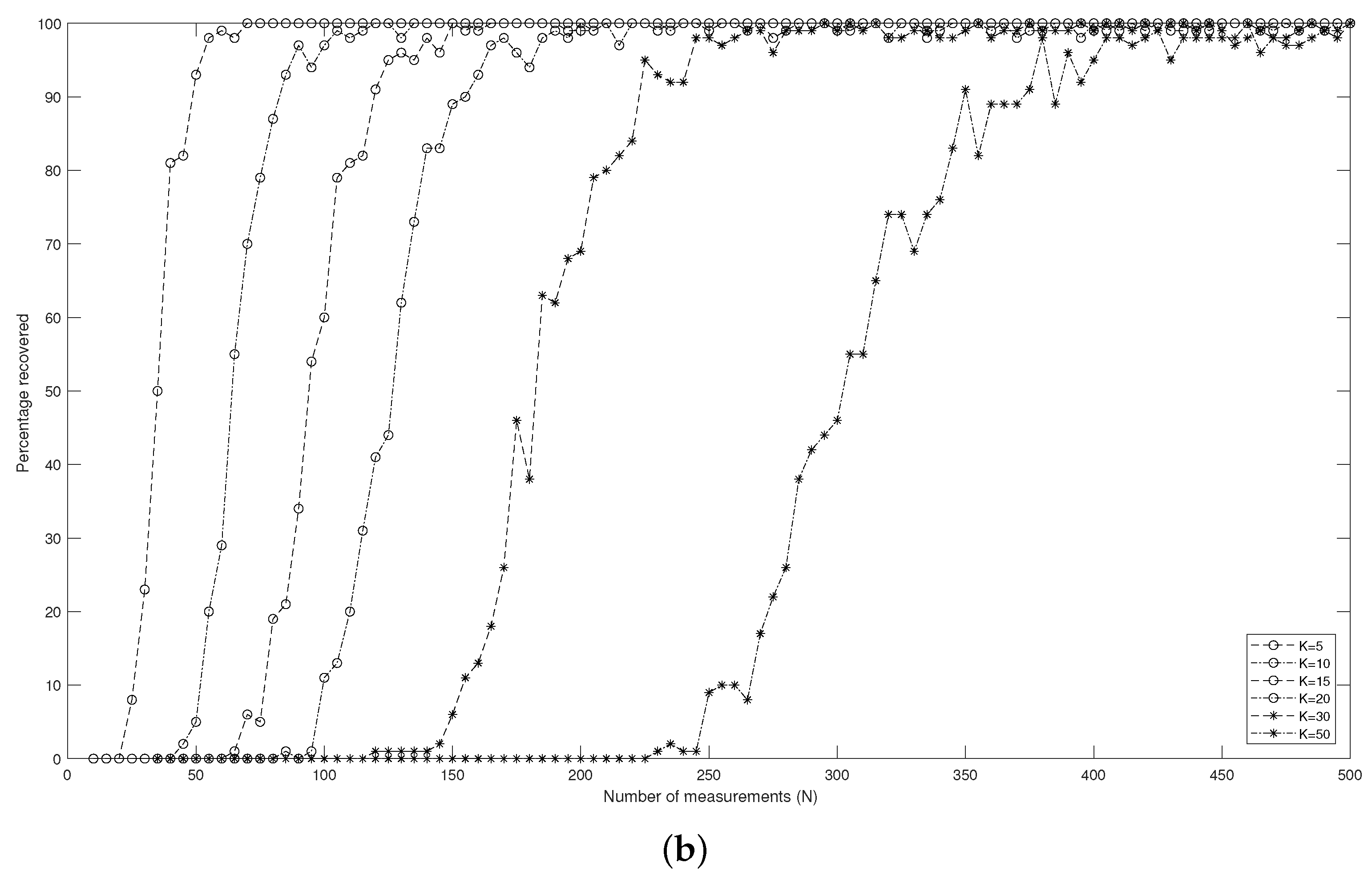
Figure 3 displays the relation between the percentage (of 100 input signals) of the support that can be determined correctly and the number N of measurements in different dimensions d. It reveals how many measurements are necessary to reconstruct a k-sparse signal $x\in {\mathbb{R}}^d$ with a high probability. A percentage equal to $100\%$ means that support for all 100 input signals can be found. That is to say, the support of the input signal can be exactly recovered. Furthermore, Figure 3 indicates that to guarantee the success of recovering the target signal, the number N of the measurements must increase when the sparsity level k increases.

The numerical experiments show that the RMP is efficient for the recovery of the sparse signals even in the noised case. The RMP can determine the support of the target signal in a high-dimension Euclidean space with a high probability, if the number N is large enough.

6. Conclusions

We design the Rescaled Matching Pursuit (RMP) algorithm for the recovery of the target signal in Euclidean space with a high dimension. The RMP algorithm performs with great advantages in terms of computational complexity over other greedy-based compressive sensing algorithms, such as the OMP algorithm, since its total cost is $O\left(N\right)$ at m iterations. By using the RIP condition, we derive the convergence rate of the error between the original signal and its approximation for the RMP algorithm. Moreover, we prove that the RMP algorithm can recover the support of the original sparse signal by using an admissible matrix with a high probability. Our numerical simulation results also verify this conclusion. And, we show that the RMP can obtain a good approximation for original sparse signal under noise, namely, the RMP is stable with noise. Thus, in both theory and practice, we show that the RMP algorithm is powerful in random cases. Although the computational cost of the RMP is smaller than that of the OMP, the performance of the RMP is not better than the OMP in the deterministic case. However, in randomized cases, the two algorithms perform similarly. Thus, if the sparsity level k of the target signal is large and computational resources are limited, then the RMP with random measurements may be a good choice.

References

1. Donoho, D.L. Compressed sensing. IEEE Trans. Inf. Theory 2006, 52, 1289–1306. [Google Scholar] [CrossRef]
2. Candès, E.J.; Romberg, J.; Tao, T. Robust uncertainty principles: Exact signal reconstruction from highly incomplete frequency information. IEEE Trans. Inf. Theory 2006, 52, 489–509. [Google Scholar] [CrossRef]
3. Yuan, X.; Haimi-Cohen, R. Image compression based on compressive sensing: End-to-end comparison with JPEG. IEEE Trans. Multimed. 2020, 22, 2889–2904. [Google Scholar] [CrossRef]
4. Berger, C.R.; Wang, Z.; Huang, J.; Zhou, S. Application of compressive sensing to sparse channel estimation. IEEE Commun. Mag. 2010, 48, 164–174. [Google Scholar] [CrossRef]
5. Barranca, V.J. Reconstruction of sparse recurrent connectivity and inputs from the nonlinear dynamics of neuronal networks. J. Comput. Neurosci. 2023, 51, 43–58. [Google Scholar] [CrossRef] [PubMed]
6. Dai, W.; Sheikh, M.A.; Milenkovic, O.; Baraniuk, R.G. Compressive sensing DNA microarrays. EURASIP J. Bioinform. Syst. Biol. 2009, 2009, 162824. [Google Scholar] [CrossRef]
7. Gross, D.; Liu, Y.K.; Flammia, S.T.; Becker, S.; Eisert, J. Quantum state tomography via compressed sensing. Phys. Rev. Lett. 2010, 105, 150401. [Google Scholar] [CrossRef] [PubMed]
8. Candès, E.J.; Wakin, M.B. An introduction to compressive sampling. IEEE Signal Proc. Mag. 2008, 25, 21–30. [Google Scholar] [CrossRef]
9. Candès, E.J.; Tao, T. Decoding by linear programming. IEEE Trans. Inf. Theory 2005, 51, 4203–4215. [Google Scholar] [CrossRef]
10. Cai, T.T.; Zhang, A.R. Sparse representation of a polytope and recovery of sparse signals and low-rank matrices. IEEE Trans. Inf. Theory 2014, 60, 122–132. [Google Scholar] [CrossRef]
11. Kim, S.J.; Koh, K.; Lustig, M.; Boyd, S.; Gorinevsky, D. An interior-point method for large-scale 1-regularized least squares. IEEE J. Sel. Top. Signal Process. 2007, 1, 606–617. [Google Scholar] [CrossRef]
12. Candès, E.J.; Tao, T. Near-optimal signal recovery from random projections: Universal encoding strategies? IEEE Trans. Inf. Theory 2006, 52, 5406–5425. [Google Scholar] [CrossRef]
13. Aziz, A.; Salim, A.; Osamy, W. Sparse signals reconstruction via adaptive iterative greedy algorithm. Int. J. Comput. Appl. 2014, 90, 5–11. [Google Scholar]
14. Goyal, P.; Singh, B. Greedy algorithms for sparse signal recovery based on temporally correlated experimental data in WSNs. Arab. J. Sci. Eng. 2018, 43, 7253–7264. [Google Scholar] [CrossRef]
15. Chae, J.; Hong, S. Greedy algorithms for sparse and positive signal recovery based on bit-wise MAP detection. IEEE Trans. Signal Process. 2020, 68, 4017–4029. [Google Scholar] [CrossRef]
16. Lv, X.L.; Wan, C.R.; Bi, G.A. Block orthogonal greedy algorithm for stable recovery of block-sparse signal representations. Signal Process. 2010, 90, 3265–3277. [Google Scholar] [CrossRef]
17. Tropp, J.A.; Gilbert, A.C. Signal recovery from random measurements via orthogonal matching pursuit. IEEE Trans. Inf. Theory 2007, 53, 4655–4666. [Google Scholar] [CrossRef]
18. Huber, P.J. Projection pursuit. Ann. Stat. 1985, 13, 435–475. [Google Scholar] [CrossRef]
19. DeVore, R.A.; Temlyakov, V.N. Some remarks on greedy algorithms. Adv. Comput. Math. 1996, 5, 173–187. [Google Scholar] [CrossRef]
20. Barron, A.R.; Cohen, A.; Dahmen, W.; DeVore, R.A. Approximation and learning by greedy algorithms. Ann. Stat. 2008, 36, 64–94. [Google Scholar] [CrossRef]
21. Pati, Y.C.; Rezaiifar, R.; Krishnaprasad, P.S. Orthogonal matching pursuit: Recursive function approximation with applications to wavelet decomposition. In Proceedings of the 27th Asilomar Conference on Signals, Systems and Computers, Pacific Grove, CA, USA, 1–3 November 1993; Volume 1, pp. 40–44. [Google Scholar]
22. Shao, C.F.; Wei, X.J.; Ye, P.X.; Xing, S. Efficiency of orthogonal matching pursuit for group sparse recovery. Axioms 2023, 12, 389. [Google Scholar] [CrossRef]
23. Davis, G.; Mallat, S.; Avellaneda, M. Adaptive greedy approximations. Constr. Approx. 1997, 13, 57–98. [Google Scholar] [CrossRef]
24. Zhang, T. Sparse recovery with orthogonal matching pursuit under RIP. IEEE Trans. Inf. Theory 2011, 57, 6215–6221. [Google Scholar] [CrossRef]
25. Eldar, Y.C.; Kutyniok, G. Compressed Sensing: Theory and Applications; Cambridge University Press: Cambridge, UK, 2012. [Google Scholar]
26. Petrova, G. Rescaled pure greedy algorithm for Hilbert and Banach spaces. Appl. Comput. Harmon. Anal. 2016, 41, 852–866. [Google Scholar] [CrossRef]
27. Gao, Z.M.; Petrova, G. Rescaled pure greedy algorithm for convex optimization. Calcolo 2019, 56, 15. [Google Scholar] [CrossRef]
28. Guo, Q.; Liu, X.H.; Ye, P.X. The learning performance of the weak rescaled pure greedy algorithms. J. Inequal. Appl. 2024, 2024, 30. [Google Scholar] [CrossRef]
29. Zhang, W.H.; Ye, P.X.; Xing, S. Optimality of the rescaled pure greedy learning algorithms. Int. J. Wavelets Multiresolut. Inf. Process. 2023, 21, 2250048. [Google Scholar] [CrossRef]
30. Jiang, B.; Ye, P.X. Efficiency of the weak rescaled pure greedy algorithm. Int. J. Wavelets Multiresolut. Inf. Process. 2021, 19, 2150001. [Google Scholar] [CrossRef]
31. Zhang, W.H.; Ye, P.X.; Xing, S.; Xu, X. Optimality of the approximation and learning by the rescaled pure super greedy algorithms. Axioms 2022, 11, 437. [Google Scholar] [CrossRef]
32. Nguyen, H.; Petrova, G. Greedy strategies for convex optimization. Calcolo 2017, 54, 207–224. [Google Scholar] [CrossRef]
33. Temlyakov, V.N. Greedy Approximation; Cambridge University Press: Cambridge, UK, 2011. [Google Scholar]
34. Shao, C.F.; Chang, J.C.; Ye, P.X.; Zhang, W.H.; Xing, S. Almost optimality of the orthogonal super greedy algorithm for μ-coherent dictionaries. Axioms 2022, 11, 186. [Google Scholar] [CrossRef]
Figure 1. The recovery of an input signal for the OMP and the RMP under different sparsity levels k, different dimensions d, and different numbers of measurements N. (a) k = 40, N = 250, d = 512; (b) k = 40, N = 250, d = 1024; (c) k = 40, N = 250, d = 2048, (d) k = 125, N = 500, d = 5000.
Axioms 13 00288 g001
Figure 2. The recovery of an input signal with sparsity level k = 40 and number of measurments N = 250 via RMP in different dimensions d and different noise levels: (a) d = 512 , no noise; (b) d = 512 , Gaussian noise; (c) d = 1024 , no noise; (d) d = 1024 , Gaussian noise. The red line denotes the original signal. The blue squares stand for the approximation obtained by applying the RMP.
Axioms 13 00288 g002
Figure 3. The percentage of the support of 100 input signals being recovered correctly as a function of the number N of Bernoulli measurements for different sparsity levels k in different dimensions d via RMP: (a) d = 512 ; (b) d = 1024 .
Axioms 13 00288 g003aAxioms 13 00288 g003b
Disclaimer/Publisher’s Note: The statements, opinions and data contained in all publications are solely those of the individual author(s) and contributor(s) and not of MDPI and/or the editor(s). MDPI and/or the editor(s) disclaim responsibility for any injury to people or property resulting from any ideas, methods, instructions or products referred to in the content.