Conformal-Based Surface Morphing and Multi-Scale Representation

Abstract

This paper presents two algorithms, based on conformal geometry, for the multi-scale representations of geometric shapes and surface morphing. A multi-scale surface representation aims to describe a 3D shape at different levels of geometric detail, which allows analyzing or editing surfaces at the global or local scales effectively. Surface morphing refers to the process of interpolating between two geometric shapes, which has been widely applied to estimate or analyze deformations in computer graphics, computer vision and medical imaging. In this work, we propose two geometric models for surface morphing and multi-scale representation for 3D surfaces. The basic idea is to represent a 3D surface by its mean curvature function, H, and conformal factor function λ, which uniquely determine the geometry of the surface according to Riemann surface theory. Once we have the $(\lambda ,H)$ parameterization of the surface, post-processing of the surface can be done directly on the conformal parameter domain. In particular, the problem of multi-scale representations of shapes can be reduced to the signal filtering on the λ and H parameters. On the other hand, the surface morphing problem can be transformed to an interpolation process of two sets of $(\lambda ,H)$ parameters. We test the proposed algorithms on 3D human face data and MRI-derived brain surfaces. Experimental results show that our proposed methods can effectively obtain multi-scale surface representations and give natural surface morphing results.

1. Introduction

Mathematical geometry processing is an active research field and has found important applications in different areas, such as in computer vision, computer graphics and medical imaging. Surface morphing and multi-scale representations of 3D shapes are two important geometry processing problems. A multi-scale surface representation aims to describe a 3D shape at different levels of geometric detail. Through a multi-scale representation of the surface, micro and macro geometric information can be extracted or represented at different scales, which allows the analyzing or editing of the surface at the global or local scales effectively. For example, in medical imaging, extracting feature landmarks from anatomical structures using different geometric quantities, such as curvatures, are important. Using the multi-scale representation of the surface, salient features can be extracted at both the global and local levels of detail. The extract features can provide a more comprehensive description of the anatomical structure [1,2,3]. Besides, most existing algorithms for surface registration require huge amounts of computational cost [4,5], which is impractical in medical imaging or computer vision. With the multi-scale representations of surfaces, one can easily obtain an approximated registration at the global scale and refine the registration at the local scale. This significantly speeds up of the computation and improves the accuracy of registering localized geometric details on surfaces [6,7]. Surface morphing is another important topic in computer vision. Surface morphing refers to the process of interpolating between two geometric shapes, which has been widely applied to estimate or analyze deformations in computer graphics, computer vision and medical imaging. For example, surface morphing has been extensively applied to 3D computer animation production and video games [8]. By modeling gradual evolutionary changes of surfaces, we can smoothly transform one 3D surface into another, thus producing a continuous deformation of shape blending. Furthermore, applications of surface morphing for biological studies have also been widely studied. For example, morphing of anatomical structures, like skeletons, organs or body movements, are also essential for improving surgical visualization, medical diagnosis and analysis. Therefore, developing effective algorithms to compute multi-scale representations of 3D surfaces and model shape evolution between surfaces are of utmost important.

Throughout this paper, we propose two geometric models for surface morphing and multi-scale representations for 3D surfaces using conformal geometry. According to Riemann surface theory, a Riemann surface can be uniquely determined by its conformal factor and mean curvature up to a rigid motion. Motivated by this, in this work, we represent the Riemann surface using its conformal factor function, λ, and mean curvature function, H. The problem of finding the multi-scale representations and the morphing of surfaces can be transformed to the $(\lambda ,H)$ parameter domains. Given a Riemann surface, S, its conformal factor, λ, and mean curvature, H, can be obtained easily through the conformal parameterization of the surface. Conversely, given λ and H, we can reconstruct the corresponding Riemann surface by solving the natural frame equations on the parameter domain. For the problem of multi-scale representations of shapes, once we obtain the $(\lambda ,H)$ representation of the surface, a Fourier transform can be applied to λ and H separately, and some filtering processes can be carried out on the Fourier coefficients. Once the filtered $(\tilde{\lambda },\tilde{H})$ representation is obtained, we can restore a corresponding Riemann surface, $\tilde{S}$, that best satisfies the Gauss–Codazzi and natural frame equations. A multi-scale representation of the surface can then be obtained. On the other hand, with the $(\lambda ,H)$ representations of the surfaces, the surface morphing problem can be transformed to an interpolation process of two sets of $(\lambda ,H)$ parameters. In particular, given two Riemann surfaces, $S_1$ and $S_2$, instead of interpolating the coordinate functions of $S_1$ to $S_2$ directly, we propose to interpolate between $({\lambda }_1,H_1)$ and $({\lambda }_2,H_2)$ (which are the conformal factor and mean curvature representations of $S_1$ and $S_2$, respectively). The intermediate surfaces can then be reconstructed, which give a surface morphing between $S_1$ and $S_2$. To test the effectiveness of the proposed algorithms, we test the methods on 3D human face data and MRI-derived brain surfaces. Experimental results show that our proposed methods can effectively obtain multi-scale surface representations and give natural surface morphing results.

In short, the contributions of this paper are two-folded. First, we propose algorithms for obtaining the multi-scale representations of 3D surfaces by considering the representation of a Riemann surface using its conformal factor, λ, and mean curvature, H. By performing Fourier filtering on both λ and H, our algorithm can effectively represent a surface at different scales of geometric details. Second, we propose an algorithm for morphing between two 3D surfaces using their corresponding $(\lambda ,H)$ representation. As λ and H can fully describe the geometric information of the surfaces, a natural interpolation between two surfaces can be obtained through interpolating between the two sets of $(\lambda ,H)$ representations. Experimental results show that the proposed morphing algorithm can produce natural surface morphing results effectively.

This paper is organized as follows. In Section 2, some related work will be reported. In Section 3, some basic mathematical background will be described. The proposed algorithms for surface morphing and multi-scale representations of shapes will be explained in detail in Section 4. The numerical implementation details will be described in Section 5. We report the the experimental results in Section 6. The paper is summarized in Section 7.

2. Previous Work

Conformal parameterization has been extensively studied [9,10,11,12,13]. For example, Hurdal et al. proposed to use circle packing for computing conformal parameterization and to apply it to register human brain surfaces [14]. Gu et al. [9,10,11] proposed to compute conformal parameterization using harmonic energy minimization with holomorphic one-forms and use it for brain surface registration. The authors in [15,16] use a least squares approach to find the conformal parameterization of surfaces, in which a free boundary parameterization will be the result. By using conformal factor and curvatures, the authors in [17,18] proposed to use the shape index to measure geometric difference between hippocampal surfaces.

In computer vision, the multi-scale representations of shapes have also been widely used and studied. For example, the multi-scale representation has been applied in surface compression and progressive transmission [19,20]. Multi-scale representations of shapes have also been effectively applied in shape analysis [21,22], since the idea of multi-scale representation is to represent a surface with different scales of geometric details. For example, in [21], the authors proposed to construct a parameterization of a surface onto a simple domain, which is then used for remeshing and multi-resolution shape analysis. Cipriano et al. [23] proposed localized shape descriptors that compactly characterize regions of a surface. The basic idea of these descriptors is to use a quadratic surface to fit the original surface. Multiscale representation has also been applied to 3D surface feature extraction [24]. The basic idea is to compute the shape index of a surface at multiple scales by fitting a surface to a local neighborhood of different sizes. The maxima of surface variation, which is calculated by the variation of shape index, is chosen as the features of the 3D surfaces. Further applications of these features are used in surface registration. In computer graphics, multi-scale representation for point clouds has also been studied [25]. The authors suggested to first compute the point-based surface approximately at coarser levels, followed by an application of geometric low pass filtering. This step is repeated successively to obtain a multi-scale representation.

Various algorithms for surface morphing, which tells us how a surface evolves, have been proposed. Liu et al. [26] proposed a modified as-rigid-as possible surface morphing algorithm for surface mesh evolution, which was originally proposed by Alexa [27]. Kanai et al. [28] first partition the original and target surfaces into pieces for constructing local parameterizations, such that consistent meshes can be formed. In [29], a consistent surface controlling approach is proposed for shape optimization. By solving the optimization problem, the morphing problem is solved in the control space with some regularity and smoothness constraints. Morphing has also been applied in various fields. For example, in anatomical analysis, Rajamani et al. [30] proposed to construct a statistical model using principal component analysis (PCA) through the training objects and by using weighted least squares to fit the deformable model. A different approach to surface morphing is to create implicit functions for surfaces and to apply a smooth interpolation between these implicit functions to construct the surface morphing. Hughes [31] proposed to transform the iso-surfaces of the models and to interpolate between their corresponding Fourier transforms of the models. Turk et al. [32] combined both implicit function creation and interpolation steps to obtain the surface/volumes transformation.

3. Mathematical Background

In this section, we describe some basic mathematical concepts relevant to our algorithms.

3.1. Conformal Factor and Curvature of a Riemann Surface

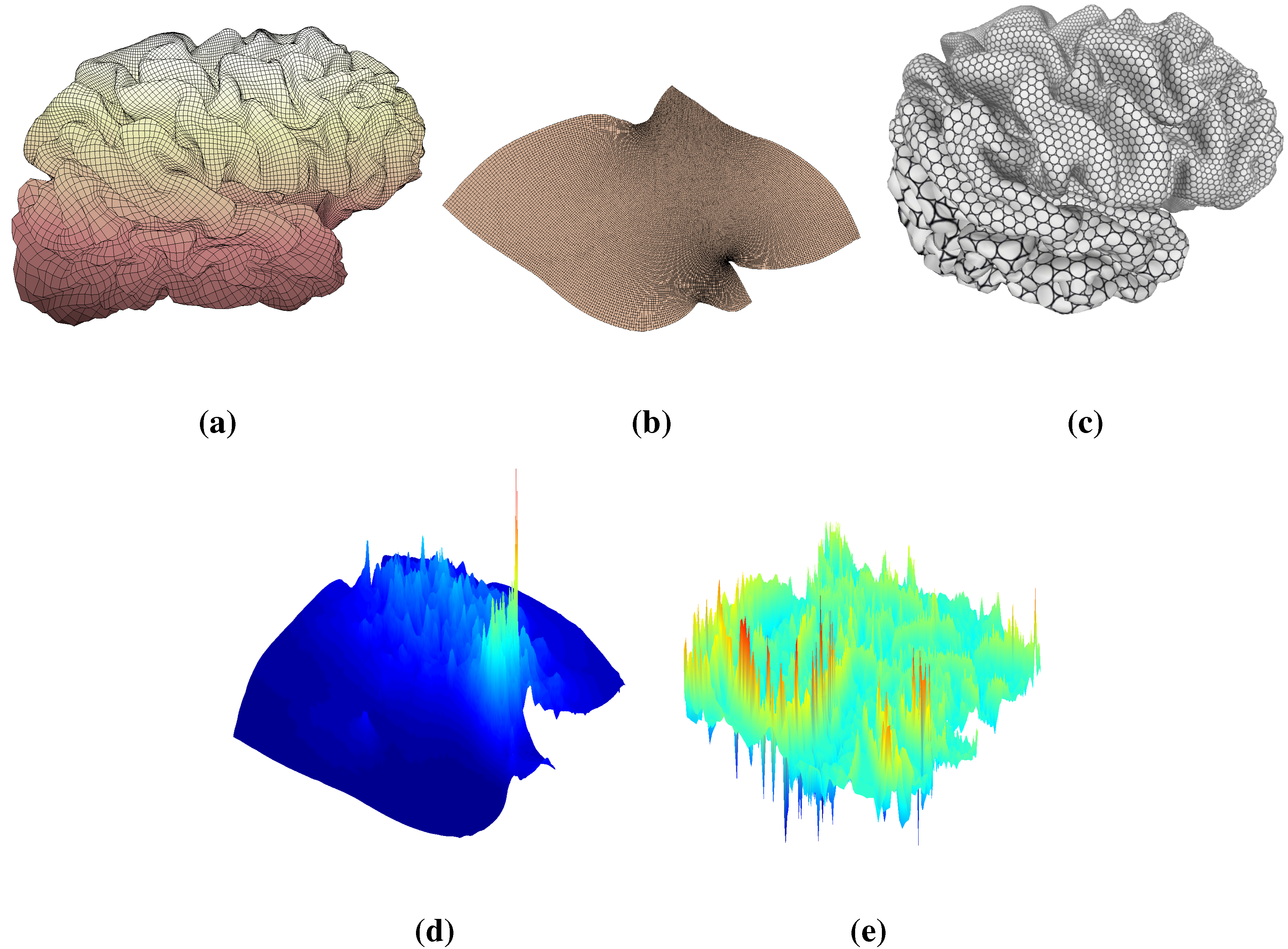
Recall that a Riemann surface, S, is an oriented manifold of dimension two with a conformal structure. Locally, every Riemann surface is Euclidean. Therefore, given two Riemann surfaces, $S_k$, $k=1,2$, they can be represented locally by:

$${\varphi }_{S_k}(x_1,x_2):U_k\in {\mathbb{R}}^2\to S_k\in {\mathbb{R}}^3,k=1,2$$

(1)

The Riemannian metric on $S_k$ can then be written as:

$$d{s}_{S_k}^2=\sum _{i,j}{g}_{i,j}^{k}d{x}^{1}d{x}^2$$

(2)

where

$$g_{i,j}^k=\frac{\partial {\varphi }_{S_k}}{\partial x}·\frac{\partial {\varphi }_{S_k}}{\partial y},k=1,2$$

(3)

With this local parameterization, for any given map $f:S_1\to S_2$, f can be represented locally by the coordinates $(x_1,x_2)$ as:

$$\tilde{f}={\varphi }_{S_2}^{-1}\circ f\circ {\varphi }_{S_1}:U_1\to U_2$$

(4)

Denote $\tilde{f}=(\widetilde{f_1},\widetilde{f_2})$, and let $v_1$ and $v_2$ be tangent vectors on $S_1$. By the mapping, f, the tangent vectors can be mapped to $f_{*}\left(v_1\right)$ and $f_{*}\left(v_2\right)$, respectively. Using this new pair of tangent vectors, a new Riemannian metric, $f^{*}(d{s}_{S_2}^2)$, defined on $S_1$, can be induced by f and $d{s}_{S_2}^2$:

$$\begin{array}{cc}\hfill f^{*}(d{s}_{S_2}^2)(v_1,v_2)& :=<f_{*}\left(v_1\right),f_{*}\left(v_2\right)>\hfill \\ & =\sum _{i,j}{g}_{i,j}^2{f}_{*}\left(v_i\right)·f_{*}\left(v_j\right)\hfill \\ & =\sum _{i,j}\left(\sum _{m,n}{g}_{mn}^2\frac{\partial \widetilde{f_i}}{\partial x^m}\frac{\partial \widetilde{f_j}}{\partial x^n}\right)v_i{v}_j\hfill \end{array}$$

(5)

With this new Riemannian metric, we say the map, f, is conformal if:

$$f^{*}(d{s}_{S_2}^2)=\lambda {(x_1,x_2)}^{2}d{s}_{S_1}^2$$

(6)

where $\lambda (x_1,x_2)$ is called the conformal factor. Then, for any parameterization $\phi :S_1=U\in {\mathbb{R}}^2\to S_2$ satisfying the Equation (6) is called a conformal parameterization. Intuitively, Equation (6) tells us that a conformal map preserves the inner product of tangent vectors up to a scaling factor, which is the conformal factor, λ. By using the properties of the inner product, it can be shown that any conformal map preserves angles.

Another important geometric quantities is the curvature of a Riemann surface. Recall the mean curvature, H, is defined as the average of the principal curvatures:

$$H=\frac{k_1+k_2}{2}$$

(7)

where $k_1$ and $k_2$ are the eigenvalues of the shape operator; the Gaussian curvature, K, is defined as the product of the principal curvatures:

$$K=k_1{k}_2$$

(8)

If the conformal parameterization $\varphi :U\in {\mathbb{R}}^2\to S$ is given, the mean curvature, H, and the Gaussian curvature, K, can be computed using the conformal factor, λ:

$$H=\frac{1}{2{\lambda }^2}\text{sign}\left(\varphi \right)|\Delta \varphi |$$

(9)

$$K=-\frac{1}{2{\lambda }^2}\Delta log\lambda$$

(10)

where $\text{sign}\left(\varphi \right)=\frac{<\Delta \varphi ,\overrightarrow{n}>}{|\Delta \varphi |}$ and $\overrightarrow{n}$ is the unit surface normal.

Figure 1 shows the results of the conformal parameterization and the computation of λ and H of a typical MRI-derived brain surface. Figure 1a shows the original brain surface mesh. Figure 1b shows the conformal parameterization of the brain, $U\in {\mathbb{R}}^2$. By defining texture coordinates with the conformal parameterization in Figure 1b, we synthesize a texture mapping onto the brain mesh, as shown in Figure 1c. Note that small circles are preserved after the texture mapping, which is consistent with our intuitive understanding of a conformal parameterization: a conformal mapping maps infinitesimal circles to infinitesimal circles up to a scaling factor. Figure 1d,e shows the corresponding conformal factor, λ, and mean curvature, H, of the brain surface.

Figure 1. Conformal parameterization of a brain cortical surface. (a) The original brain mesh; (b) the conformal parameterization onto a rectangular conformal parameter domain in ${\mathbb{R}}^2$. We then texture the brain using the parameterization obtained from (b), as shown in (c). Note that conformal parameterization maps infinitesimal circles to circles; (d,e) the conformal factor of the parameterization and the mean curvature of the brain surface, respectively.

Figure 1. Conformal parameterization of a brain cortical surface. (a) The original brain mesh; (b) the conformal parameterization onto a rectangular conformal parameter domain in ${\mathbb{R}}^2$. We then texture the brain using the parameterization obtained from (b), as shown in (c). Note that conformal parameterization maps infinitesimal circles to circles; (d,e) the conformal factor of the parameterization and the mean curvature of the brain surface, respectively.

3.2. $(\lambda ,H)$ Representation for Surface

Let S be a Riemann surface embedded in ${\mathbb{R}}^3$. Since every Riemann surface is locally Euclidean, we can find $\varphi (u,v)$, which parameterize S:

$$\varphi (u,v)=\left(X(u,v),Y(u,v),Z(u,v)\right)\in {\mathbb{R}}^3$$

(11)

Recall that the first and the second fundamental forms are:

$$\begin{array}{cc}\hfill d{s}^2& =<{\varphi }_u,{\varphi }_u>d{u}^2+2<{\varphi }_u,{\varphi }_v>dudv+<{\varphi }_v,{\varphi }_v>d{v}^2\hfill \\ \hfill II& =<{\varphi }_{uu},\overrightarrow{n}>d{u}^2+2<{\varphi }_u,\overrightarrow{n}>dudv+<{\varphi }_{vv},\overrightarrow{n}>v^2\hfill \end{array}$$

(12)

where $\overrightarrow{n}$ is the unit surface normal.

Let $z=u+iv$ ($i=\sqrt{-1}$), $dz=du+idv$, $d\overline{z}=du-idv$ $\partial z=\frac{1}{2}(\frac{\partial }{\partial u}-i\frac{\partial }{\partial v})$ and $\partial \overline{z}=\frac{1}{2}(\frac{\partial }{\partial u}+i\frac{\partial }{\partial v})$. By assuming $\varphi$ to be a conformal parameterization, we can rewrite the equations of the natural frame $({\varphi }_z,{\varphi }_{\overline{z}},\overrightarrow{n})$ as:

$$\frac{\partial }{\partial z}\left(\begin{array}{c}{\varphi }_z\\ {\varphi }_{\overline{z}}\\ \overrightarrow{n}\end{array}\right)=\left(\begin{array}{c}\frac{2}{\lambda }{\lambda }_z{\varphi }_z+\mu \overrightarrow{n}\\ \frac{{\lambda }^2}{2}H\overrightarrow{n}\\ -H{\varphi }_z-\frac{2\mu {\varphi }_{\overline{z}}}{{\lambda }^2}\end{array}\right)$$

(13)

where $\mu =<{\varphi }_{zz},\overrightarrow{n}>$. From Equation (13), we know that $\varphi$ can be determined by the conformal factor, λ, mean curvature, H, and μ. Recall the Gauss–Codazzi equation:

$${\mu }_{\overline{z}}=\frac{{\lambda }^2}{2}{H}_z$$

(14)

which can be further differentiated with respect to z to obtain:

$$\Delta \mu =\frac{1}{2}\lambda \left(2{\lambda }_z{H}_z+\lambda H_{zz}\right)$$

(15)

In other words, we can represent μ by the conformal factor, λ, and H as $\mu =\frac{1}{2}{\Delta }^{-1}\left[\lambda \left(2{\lambda }_z{H}_z+\lambda H_{zz}\right)\right]$. Therefore, given the Dirichlet boundary condition of $\varphi$ on the neighborhood, V, we can obtain $\varphi$ by solving the system of partial differential Equation (13). As a consequence, given the boundary correspondence, ${\varphi |}_{\partial S}$, S can be uniquely represented by the pair $(\lambda ,H)$.

We summarize the above discussion as the following theorem.

Theorem 1. 

($(\lambda ,H)$ representation). Let S be an open Riemann surface with mean curvature, H. Let $\varphi :U\in mathbb{R}^2$ be the conformal parameterization of S with conformal factor λ. Suppose V is a boundary neighborhood of S. Given the boundary value, ${\varphi }_{\partial V}$, of $\varphi$, S is uniquely determined by λ and H.

The $(\lambda ,H)$ representation was proposed in [33] and applied for surface inpainting in [34].

4. Methodology

In this section, we propose two algorithms, which are the multi-scale representation algorithm and the surface morphing algorithm.

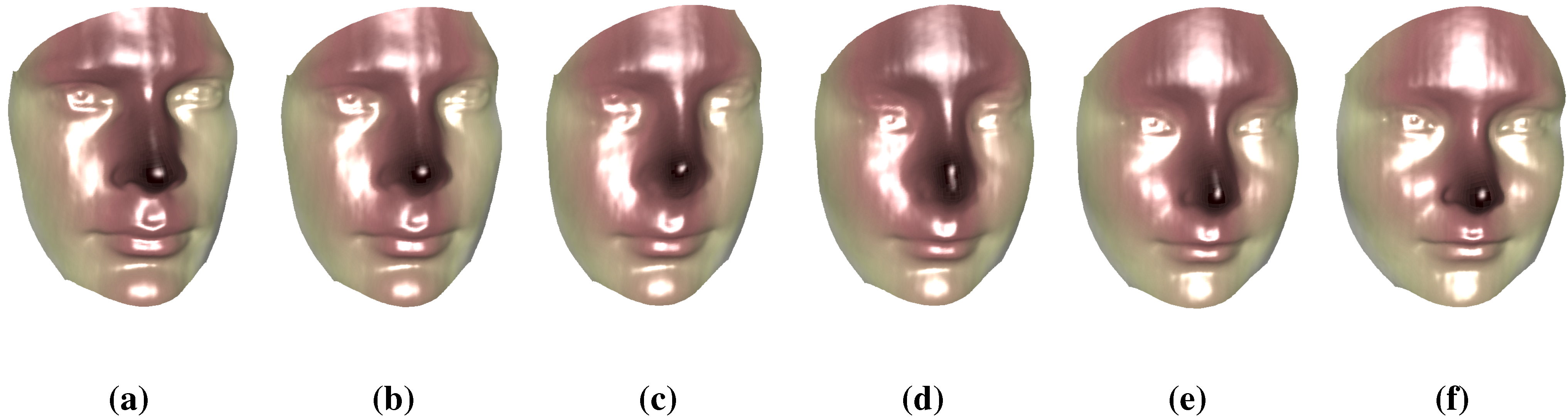
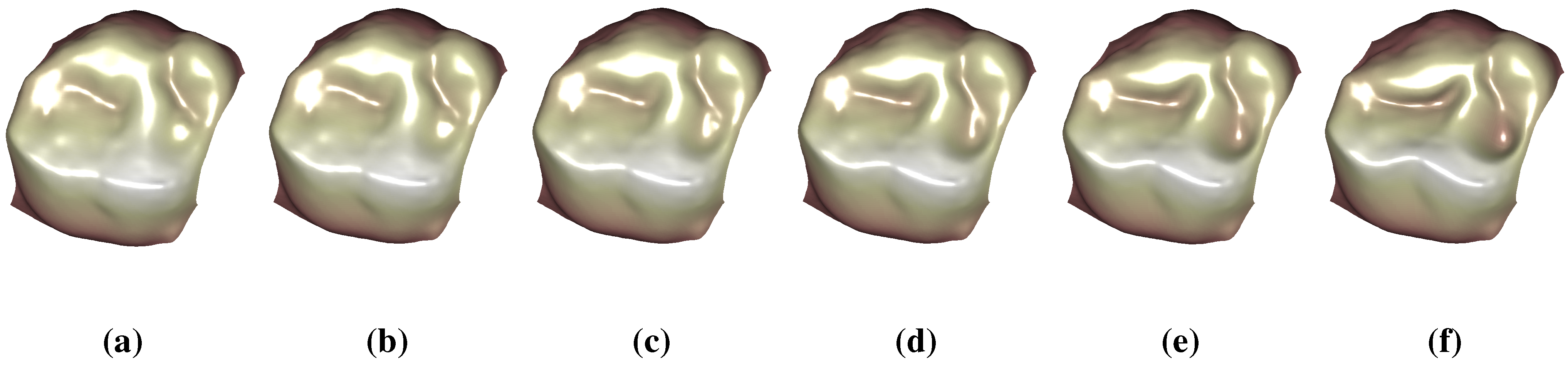
4.1. Multi-Scale Representation of Surfaces

Given a surface, S, our goal is to find a multi-scale representation of the surface that provides different scales of geometric details of the original surface. Instead of directly working on the coordinate functions of the surface embedded in ${\mathbb{R}}^3$, our proposed algorithm considers the $(\lambda ,H)$ representation of the surface. We first obtain a rectangular conformal parameterization $U=[-T_1,T_1]\times [-T_2,T_2]\in {\mathbb{R}}^2$ of the surface, S. By using Equations (6) and (9), we can calculate the corresponding λ and H of the surface, S. By viewing different scales of geometric details as different scales of noises, the main idea of our algorithm is to apply the traditional denoising method on the geometric quantities, λ and H, to find the multi-scale representation of the surface. In other words, for a specific scale, K, we first apply a Fourier transform on λ and H, respectively, in U to obtain two sets of Fourier coefficients, $C^{\lambda }$ and $C^H$:

$$C_{m,n}^{\lambda }=\frac{1}{4\pi }{\int }_{-T_2}^{T_2}{\int }_{-T_1}^{T_1}\lambda (x,y)e^{-i\pi jx/T_1}{e}^{-i\pi ky/T_2}dxdy$$

(16)

$$C_{m,n}^H=\frac{1}{4\pi }{\int }_{-T_2}^{T_2}{\int }_{-T_1}^{T_1}H(x,y)e^{-i\pi jx/T_1}{e}^{-i\pi ky/T_2}dxdy$$

(17)

where the original λ and H can be expressed by the Fourier expansion as follows:

$$\lambda (x,y)=\sum _{m,n-\infty }^{\infty }{C}_{m,n}^{\lambda }{e}^{i\pi mx/T_1}{e}^{j\pi ny/T_2}$$

(18)

$$H(x,y)=\sum _{m,n-\infty }^{\infty }{C}_{m,n}^H{e}^{i\pi mx/T_1}{e}^{j\pi ny/T_2}$$

(19)

Treating as denoising white noise in signal processing, we consider coefficients with magnitude smaller than K as pure noise and set them to zero. The corresponding truncated Fourier expansions of λ and H form a new pair of denoised $(\tilde{\lambda },\tilde{H})$ parameterization, which represents a “denoised” surface with some of the geometric details removed. Using the $(\lambda ,H)$ reconstruction scheme, we can get the corresponding surface, $\tilde{S}$, of scale K as required.

In summary, the proposed multi-scale representation algorithm can be described as follows:

Algorithm 1: Multi-scale representation of a surface.

Input: Surface S, scale K Output: Surface $\tilde{S}$ of scale K 1  Conformally parameterize S into $U=[-T_1,T_1]\times [-T_2,T_2]\in {\mathbb{R}}^2$; 2  Compute conformal factor λ and mean curvature H; 3  Apply Fourier transform on λ and H to get $C_{m,n}^{\lambda }$ and $C_{m,n}^H$, respectively; 4  Truncate the Fourier coefficients less than the bound, K, to obtain ${\tilde{C}}_{m,n}^{\lambda }$, ${\tilde{C}}_{m,n}^H$; 5  Apply inverse Fourier transform to get $\tilde{\lambda }$ and $\tilde{H}$; 6  Carry out $(\lambda ,H)$ reconstruction scheme to get $\tilde{S}$ of scale K.

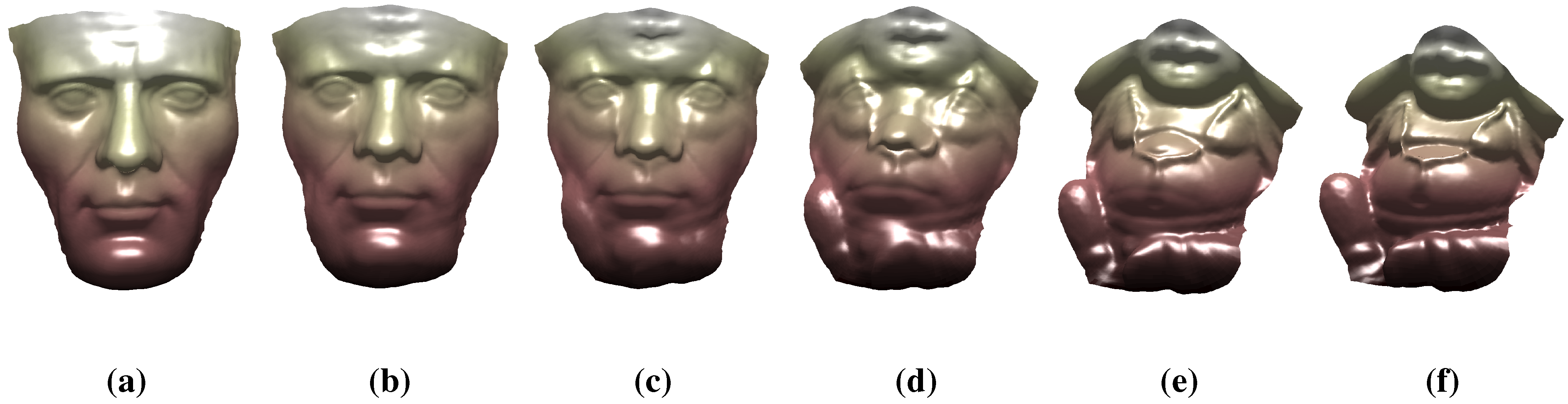
4.2. Surface Morphing

Given two surfaces, $S_1$ and $S_2$, the process of finding the evolution from surface $S_1$ to $S_2$ is called surface morphing. In other words, our goal is to compute every $S\left(t\right)$, where $t\in [0,1]$, $S\left(0\right)=S_1$ and $S\left(1\right)=S_2$. To achieve this, we again consider the $(\lambda ,H)$ representation rather than the ${\mathbb{R}}^3$ space directly. Let $\partial S_i$ be the boundary of surface $S_i$, $i=1,2$. By assuming that we already have the boundary matching obtained from arc-length parameterization or some other curve matching algorithms [35], we interpolate every point on $\partial S_1$ linearly in ${\mathbb{R}}^3$ to corresponding points in $\partial S_2$:

$$\left(\begin{array}{c}x\left(t\right)\\ y\left(t\right)\\ z\left(t\right)\end{array}\right)=(1-t)\left(\begin{array}{c}{x}_1\\ y_1\\ z_1\end{array}\right)+t\left(\begin{array}{c}{x}_2\\ y_2\\ z_2\end{array}\right)$$

(20)

where ${\left(x_1,y_1,z_1\right)}^T\in \partial S_1$ and ${\left(x_2,y_2,z_2\right)}^T\in \partial S_2$. From this, we obtain a simple boundary morphing approximation from surfaces $S_1$ to $S_2$. Next, we compute rectangular conformal parameterization for both surfaces $S_1$ and $S_2$, respectively, as in Algorithm 1. Two pairs, $({\lambda }_1,H_1)$ and $({\lambda }_2,H_2)$, corresponding to surfaces $S_1$ and $S_2$ can then be obtained. To approximate the evolution naturally, we propose to morph the geometric quantities, λ and H, from the pair, $({\lambda }_1,H_1)$ to $({\lambda }_2,H_2)$, by simply linear interpolation:

$$\lambda \left(t\right)=(1-t){\lambda }_1+t{\lambda }_2$$

(21)

$$H\left(t\right)=(1-t)H_1+t{H}_2$$

(22)

Substituting $t\in [0,1]$ with different values, we get a sequence of pairs $\left(\lambda \right(t),H(t\left)\right)$ with boundary constraint $\partial S\left(t\right)$. By using the $(\lambda ,H)$ reconstruction algorithm, the corresponding surface $S\left(t\right)$, which best fits the Gauss–Codazzi and natural frame equations, can be constructed. This gives a morphing surface at time $t\in [0,1]$.

Our proposed morphing algorithm can be summarized as follows:

Algorithm 2: Morphing of surfaces.

Input: Surface $S_1$ and $S_2$, time t Output: Intermediate surface $S\left(t\right)$ between $S_1$ and $S_2$ 1  Obtain the boundary matching between $S_1$ and $S_2$; 2  Compute the boundary morphing $\partial S\left(t\right)$ by linear interpolation pointwisely; 3  Compute conformal parameterization for both $S_1$ and $S_2$; 4  Compute $({\lambda }_1,H_1)$ and $({\lambda }_2,H_2)$ corresponding to $S_1$ and $S_2$, respectively; 5  Use the $(\lambda ,H)$ reconstruction algorithm with $\left(\lambda \right(t),H(t\left)\right)$ and $\partial S\left(t\right)$ to compute $S\left(t\right)$.

5. Numerical Algorithms

In this section, we discuss the numerical implementation of the algorithms we proposed in this paper. Firstly, we will briefly describe how we obtain the $(\lambda ,H)$ representation and the implementation of the reconstruction scheme of the surface, S, with the given conformal factor, λ, and mean curvature, H. Secondly, we will explain how the algorithms for multi-scale representation and surface morphing proposed in the previous section can be implemented.

5.1. Numerical Implementation of the $(\lambda ,H)$ Representation and Surface Reconstruction

We basically follow the numerical implementation in [34]. Given a surface, S, the conformal parameterization can be obtained by using some well-established conformal parameterization algorithms [9,10,11,13,14]. By applying the algorithm proposed in [36], we obtain the rectangular conformal parameterization $U=[0,1]\times [0,T]\in {\mathbb{R}}^2$ of the surface, S. Denote the discretized parameterization domain, U, to be:

$$U_{ij}=(ih,Tjh),h=\frac{1}{N},0\le i\le N,0\le j\le N$$

(23)

Correspondingly, we have:

$${\varphi }_{ij}=\varphi \left(U_{ij}\right)H_{ij}=H\left(U_{ij}\right)\text{and}{\lambda }_{ij}=\lambda \left(U_{ij}\right)$$

(24)

To obtain the conformal factor, ${\lambda }_{ij}$, recall that a conformal parameterization, $\varphi$, preserves the first fundamental form up to the conformal factor. Therefore, we can approximate the discrete conformal factor, ${\lambda }_{ij}$, by:

$$\begin{array}{cc}\hfill {\lambda }_{ij}& =<\frac{\partial \varphi \left(U_{ij}\right)}{\partial z},\frac{\partial \varphi \left(U_{ij}\right)}{\partial \overline{z}}>\hfill \\ & \approx \frac{1}{2}\left[{\left|\frac{{\varphi }_{i+1,j}-{\varphi }_{i-1,j}}{2h}\right|}^2+{\left|\frac{{\varphi }_{i,j+1}-{\varphi }_{i,j-1}}{2h}\right|}^2\right]\hfill \end{array}$$

(25)

For the mean curvature, $H_{ij}$, we consider Equation (9):

$$H_{ij}=H\left(U_{ij}\right)=\frac{1}{2{\lambda }_{ij}}\text{sign}\left({\varphi }_{ij}\right)|\Delta {\varphi }_{ij}|$$

(26)

where we approximate:

$$\Delta {\varphi }_{ij}=\frac{{\varphi }_{i+1,j}+{\varphi }_{i-1,j}-4{\varphi }_{i,j}+{\varphi }_{i,j+1}+{\varphi }_{i,j-1}}{h^2}$$

(27)

$$\text{sign}\left({\varphi }_{ij}\right)=\text{sign}(<\Delta {\varphi }_{ij},\overrightarrow{n_{ij}}>)$$

(28)

$$\overrightarrow{n_{ij}}=\left(\frac{{\varphi }_{i+1,j}-{\varphi }_{i-1,j}}{2h}\right)\times \left(\frac{{\varphi }_{i,j+1}-{\varphi }_{i,j-1}}{2h}\right)/∥\left(\frac{{\varphi }_{i+1,j}-{\varphi }_{i-1,j}}{2h}\right)\times \left(\frac{{\varphi }_{i,j+1}-{\varphi }_{i,j-1}}{2h}\right)∥$$

(29)

If we are given the $(\lambda ,H)$ representation, we can reconstruct the surface, S, by solving Equation (13). Let $({\left({\varphi }_z\right)}_{ij},{\left({\varphi }_{\overline{z}}\right)}_{ij},{\overrightarrow{n}}_{ij})=(P_{ij},Q_{ij},N_{ij})$ be the natural frame at $U_{ij}$. Similarly as above, we can discretize the system into the following:

$$\frac{1}{2h}\left(\begin{array}{c}(P_{i+1,j}-P_{i-1,j})-\sqrt{-1}(P_{i,j+1}-P_{i,j-1})\\ (Q_{i+1,j}-Q_{i-1,j}-\sqrt{-1}(Q_{i,j+1}-Q_{i,j-1})\\ 2h{N}_{ij}\end{array}\right)=\left(\begin{array}{c}\frac{2}{{\lambda }_{ij}}{\left({\lambda }_z\right)}_{ij}{P}_{ij}+{\mu }_{ij}{N}_{ij}\\ \frac{{\lambda }_{ij}^2}{2}{H}_{ij}{N}_{ij}\\ -H_{ij}{P}_{ij}-\frac{2{\mu }_{ij}{Q}_{ij}}{{\lambda }_{ij}^2}\end{array}\right)$$

(30)

We solve Equation (30) by the least squares method.

Once we obtain $(P_{ij},Q_{ij},N_{ij})$ by solving Equation (30), we can reconstruct the surface by solving:

$$\frac{1}{2h}\left(\begin{array}{c}{\varphi }_{i+1,j}-{\varphi }_{i-1,j}\\ {\varphi }_{i,j+1}-{\varphi }_{i,j-1}\end{array}\right)=\left(\begin{array}{c}(P_{ij}+Q_{ij})/2\\ \sqrt{-1}(P_{ij}-Q_{ij})/2\end{array}\right)$$

(31)

For more details, please refer to [34].

5.2. Numerical Implementation of the Multi-Scale Representation of a Surface

Given a surface, S, Algorithm 1 produces a surface, $\tilde{S}$, with a coarser scale of geometric details. Since we have chosen the conformal parameterization domain, U, to be a rectangle, conformal factor λ and mean curvature H are well defined on U, as well. Then, by using the discrete fast Fourier transform (DFT), we are able to get $C_{ij}^{\lambda }$ and $C_{ij}^H$ immediately. The truncation process is simply by:

$$\begin{array}{c}\hfill C_{ij}^{\lambda }=0\text{if}\left|C_{ij}^{\lambda }\right|\le K\\ \hfill C_{ij}^H=0\text{if}\left|C_{ij}^H\right|\le K\end{array}$$

(32)

By using inverse discrete fast Fourier transform (IDFT) on the updated $C_{ij}^{\lambda }$ and $C_{ij}^H$, $(\tilde{\lambda },\tilde{H})$ can be obtained.

5.3. Numerical Implementation of Surface Morphing

In Algorithm 2, there are many ways to obtain meaningful boundary registration results. Here, we discuss the method of arc-length parameterization for boundary matching that works very well, as shown in our experimental results in the next section.

Given two surfaces, $S_1$ and $S_2$, with boundaries $\partial S_1$ and $\partial S_2$, denote the vertices on boundaries to be ${\left\{v_1\left(k\right)\right\}}_k$ and ${\left\{v_2\left(h\right)\right\}}_h$, respectively. We assume we have labeled a few point-correspondences:

$$v_1\left(p_i\right)=v_2\left(q_i\right),1\le p_i\le I,I\le q_i\le J,i=1:N$$

(33)

Consider the line segments $[v_1\left(p_i\right),v_1(p_i+1),...,v_1\left(p_{i+1}\right)]\subset {\left\{v_1\left(k\right)\right\}}_k\subset {\mathbb{R}}^3$ and $[v_2\left(q_i\right),v_2(q_i+1),...,$ $v_2\left(q_{i+1}\right)]\subset {\left\{v_2\left(h\right)\right\}}_h\subset {\mathbb{R}}^3$; two arc-length parameterizations, $(\alpha ,f_1\left(\alpha \right))$ and $(\beta ,f_2\left(\beta \right))$, can be obtained, where $p_i\le \alpha \le p_{i+1}$, $q_i\le \beta \le q_{i+1}$, $f_1\left(\alpha \right)=v_1\left(\alpha \right)$ and $f_2\left(\beta \right)=v_2\left(\beta \right)$, respectively. To obtain the boundary registration, we define $P\left(\alpha \right)$ as:

$$P\left(\alpha \right)=f_2\left(q_i+(q_{i+1}-q_i)\frac{\alpha -p_i}{p_{i+1}-p_i}\right)$$

(34)

where $P\left(\alpha \right)\in {\mathbb{R}}^3$. By substituting α, such that $p_i\le \alpha \le p_{i+1}$, we can obtain the corresponding position of each $v_1\left(\alpha \right)\in {\left\{v_1\left(k\right)\right\}}_k$ on $\partial S_2$.

6. Experimental Results

We have tested our multi-scale algorithm and morphing algorithm on both synthetic data and real medical data. In the following subsections, the experimental results of the proposed algorithms are reported.

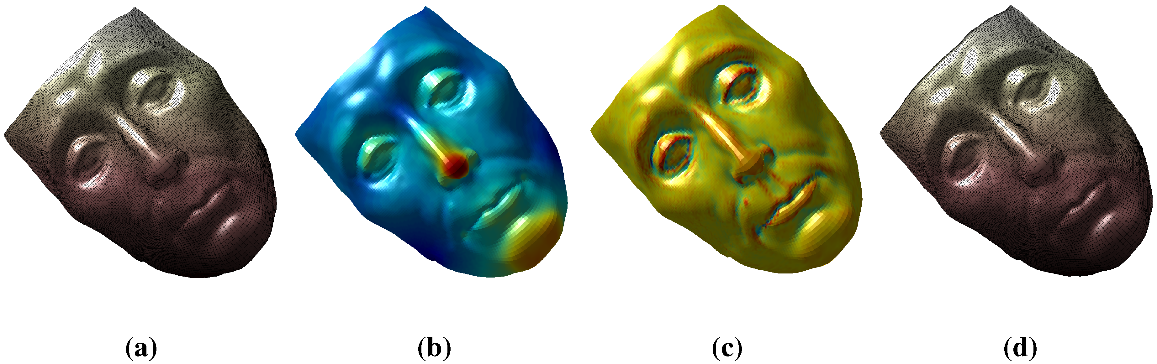
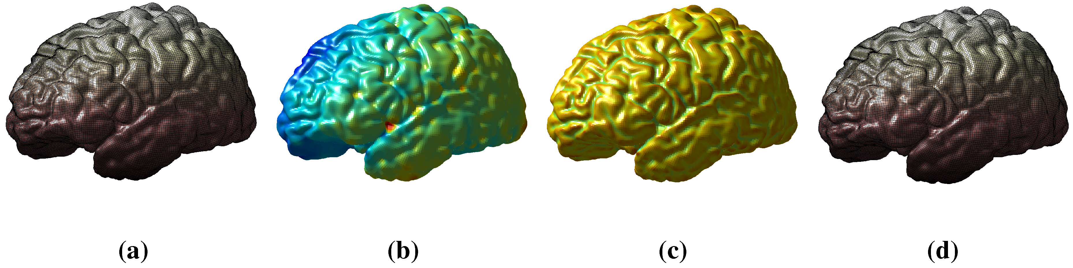
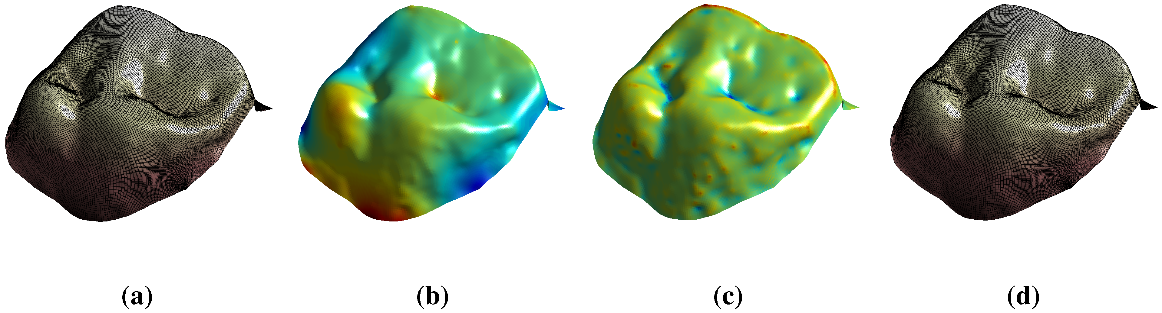
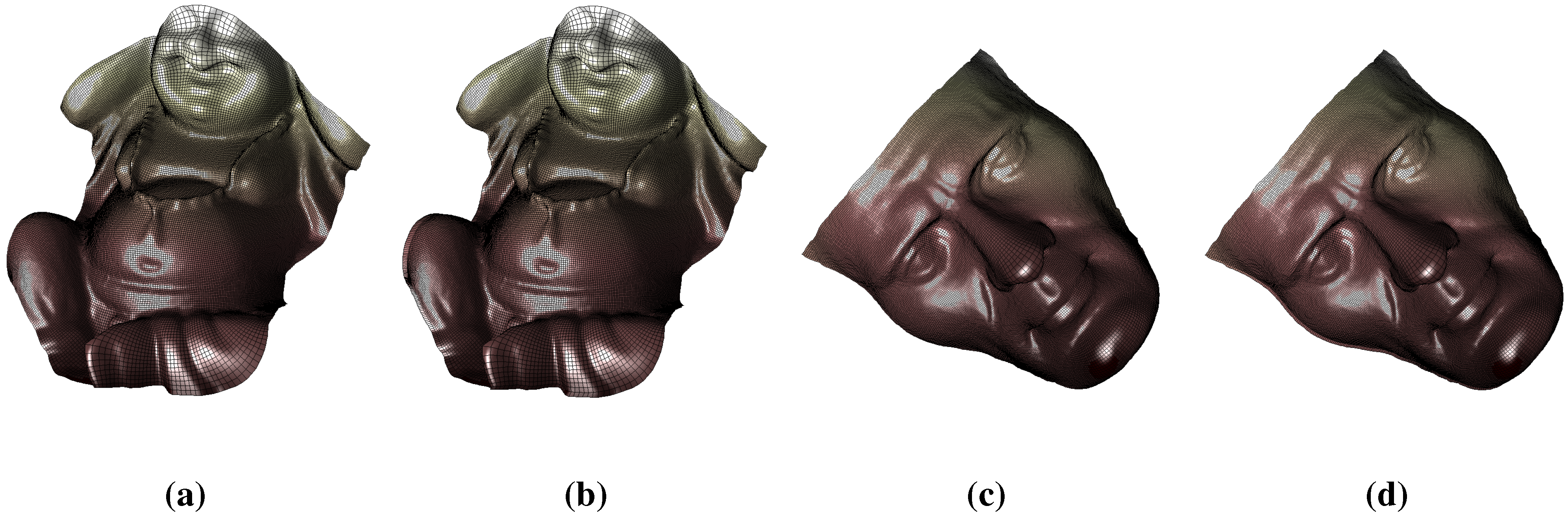
6.1. Surface Reconstruction

Our proposed algorithms depend on the $(\lambda ,H)$ representations of the Riemann surfaces. To examine how effective and accurate this geometric representation can represent the surface, we consider the $(\lambda ,H)$ representation of human faces, a brain cortical surface, a teeth surface and a partition of the Buddha surface. Figure 2a shows the original human face. We parameterize the surface onto the 2D rectangular conformal parameter domain and compute the conformal factor. The conformal factor is visualized as the colormap on the surface, which is shown in Figure 2b. The mean curvature of the surface is shown in Figure 2c. The conformal factor and mean curvature determine the surface. In Figure 2d, we reconstruct the surface from the conformal factor and mean curvature. Note that the surface closely resembles the original surface in (a). We also examine the $(\lambda ,H)$ representations for another human face, the brain cortical surface, the teeth surface and the Buddha surface, as shown in Figure 3, Figure 4 and Figure 5, respectively. Again, the $(\lambda ,H)$ representations can accurately represent the surfaces. Table 1 shows the summary of the reconstruction error of each example. We measure the reconstruction error by using the maximum distance between the original surfaces and the corresponding reconstructed surfaces in the L2sense. Since the surfaces in our experiment are at different scales, we also measure the relative error for each example by using the maximum L2 error over the square root of the surface area. As shown in the fourth column in the table, our reconstruction algorithm produces a small relative error of around 1%, which is visually unobservable. The result shows that using $(\lambda ,H)$ representations, the surfaces reconstructed closely resemble the original ones.

Figure 2. $(\lambda ,H)$ representation of a human face. (a) shows the original mesh of a face. By finding the conformal parameterization of the human face to a rectangular conformal parameter domain in ${\mathbb{R}}^2$, we calculate the conformal factor, as shown in (b)/ (c) The mean curvature of the human face. By using λ and H, we can reconstruct the human face, as shown in (d).

Figure 2. $(\lambda ,H)$ representation of a human face. (a) shows the original mesh of a face. By finding the conformal parameterization of the human face to a rectangular conformal parameter domain in ${\mathbb{R}}^2$, we calculate the conformal factor, as shown in (b)/ (c) The mean curvature of the human face. By using λ and H, we can reconstruct the human face, as shown in (d).

Figure 3. $(\lambda -H)$ representation of a human brain. (a) The original mesh of a brain. By finding the conformal parameterization of the brain to a rectangular conformal parameter domain, we calculate the conformal factor, as shown in (b). (c) The mean curvature of the brain. By using λ and H, we can reconstruct the brain, as shown in (d).

Figure 3. $(\lambda -H)$ representation of a human brain. (a) The original mesh of a brain. By finding the conformal parameterization of the brain to a rectangular conformal parameter domain, we calculate the conformal factor, as shown in (b). (c) The mean curvature of the brain. By using λ and H, we can reconstruct the brain, as shown in (d).

Figure 4. $(\lambda ,H)$ representation of a human tooth. (a) The original mesh of a tooth. By finding the conformal parameterization of the tooth to a rectangular conformal parameter domain, we calculate the conformal factor, as shown in (b). (c) The mean curvature of the tooth. By using λ and H, we can reconstruct the tooth, as shown in (d).

Figure 4. $(\lambda ,H)$ representation of a human tooth. (a) The original mesh of a tooth. By finding the conformal parameterization of the tooth to a rectangular conformal parameter domain, we calculate the conformal factor, as shown in (b). (c) The mean curvature of the tooth. By using λ and H, we can reconstruct the tooth, as shown in (d).

Figure 5. $(\lambda ,H)$ reconstruction of surfaces. (a) The original mesh of a partition of the Buddha surface. We reconstruct the surface using the corresponding λ and H in (b). (c) The original mesh of another human face surface. By using λ and H, we can reconstruct the face, as shown in (d).

Figure 5. $(\lambda ,H)$ reconstruction of surfaces. (a) The original mesh of a partition of the Buddha surface. We reconstruct the surface using the corresponding λ and H in (b). (c) The original mesh of another human face surface. By using λ and H, we can reconstruct the face, as shown in (d).

Table 1. Summary of the $\lambda -H$ reconstruction error.

Surface	Max L2 error	Mean L2 error	Max (L2/$\sqrt{\mathbf{Area}}$) error
Human face	3.0033	1.0771	0.0167
Human face 2	2.5706	0.7239	0.0150
Cortical surface	2.2157	0.5967	0.0114
Teeth surface	0.1189	0.0329	0.0098
Buddha surface	8.7897	2.1967	0.0183

Table 1. Summary of the $\lambda -H$ reconstruction error.

Surface	Max L2 error	Mean L2 error	Max (L2/$\sqrt{\mathbf{Area}}$) error
Human face	3.0033	1.0771	0.0167
Human face 2	2.5706	0.7239	0.0150
Cortical surface	2.2157	0.5967	0.0114
Teeth surface	0.1189	0.0329	0.0098
Buddha surface	8.7897	2.1967	0.0183

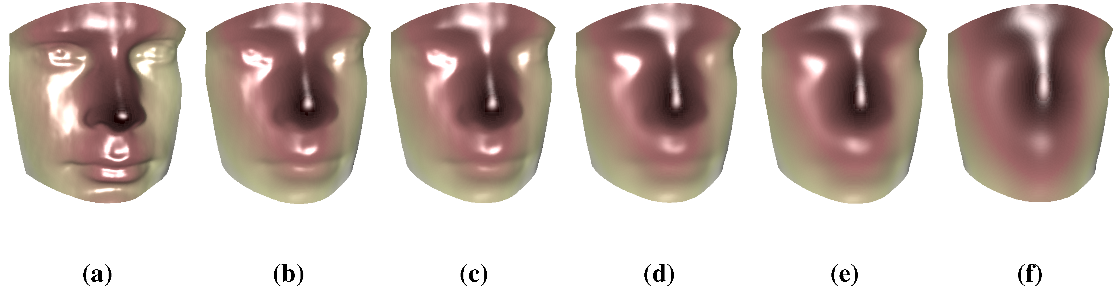
6.2. Multi-Scale Representation of Surfaces

We first test our proposed surface multi-scale representation algorithm on a synthetic human surface. Figure 6a shows the original surface mesh of a human face model. Using Algorithm 1, we compute different levels of geometric details, as shown in Figure 6b–f. The approximation levels decrease from Figure 6b to Figure 6f by increasing the bound, K, in the algorithm. In other words, we truncated more and more terms in the Fourier expansion of both λ and H. Therefore, facial characteristics, like eyes, nose and mouth, are fading gradually.

We have also tested our multi-scale algorithm on a human brain surface, which has a more complicated surface geometric structure. Figure 7a shows the original brain surface. There are lots of different sizes and lengths of sulci located on the brain surface. By applying Algorithm 1 to the brain surface, we obtain the multi-scale representation, as shown in Figure 7b–i. Similarly, the approximation levels decreases from Figure 7b to Figure 7i by increasing the bound, K, in Algorithm 1. Note that from Figure 7b to Figure 7i, geometric features, like the sulci, are fading out. This is consistent with our reduction in the number of effective Fourier coefficients. This also shows that our algorithm works well on complicated surfaces and provides a multi-scale representation of different surfaces.

Figure 6. Result of the multi-scale representation of a human face surface. (a) The original human face. (b–f) The multi-scale representation of the face obtained from the proposed algorithm. The approximation levels of the multi-scale representation decreases from the fine-scale (see (b)) to the coarse-scale (see (f)). Note that from (b) to (f), the facial characteristics, such as eyes, nose and mouth, are fading out. This is consistent with our algorithm, which coarsens the $(\lambda ,H)$ representation throughout the process.

Figure 6. Result of the multi-scale representation of a human face surface. (a) The original human face. (b–f) The multi-scale representation of the face obtained from the proposed algorithm. The approximation levels of the multi-scale representation decreases from the fine-scale (see (b)) to the coarse-scale (see (f)). Note that from (b) to (f), the facial characteristics, such as eyes, nose and mouth, are fading out. This is consistent with our algorithm, which coarsens the $(\lambda ,H)$ representation throughout the process.

Figure 7. Result of the multi-scale representation of a brain surface. (a) The original brain surface. (b–i) The multi-scale representation of the brain obtained from the proposed algorithm. The approximation levels of the multi-scale representation decreases from the fine-scale (see (b)) to the coarse-scale (see (i)). Note that from (b) to (i), geometric characteristics, like sulci on the brain, are fading out. This is consistent with our algorithm, which coarsens the $(\lambda ,H)$ representation throughout the process.

Figure 7. Result of the multi-scale representation of a brain surface. (a) The original brain surface. (b–i) The multi-scale representation of the brain obtained from the proposed algorithm. The approximation levels of the multi-scale representation decreases from the fine-scale (see (b)) to the coarse-scale (see (i)). Note that from (b) to (i), geometric characteristics, like sulci on the brain, are fading out. This is consistent with our algorithm, which coarsens the $(\lambda ,H)$ representation throughout the process.

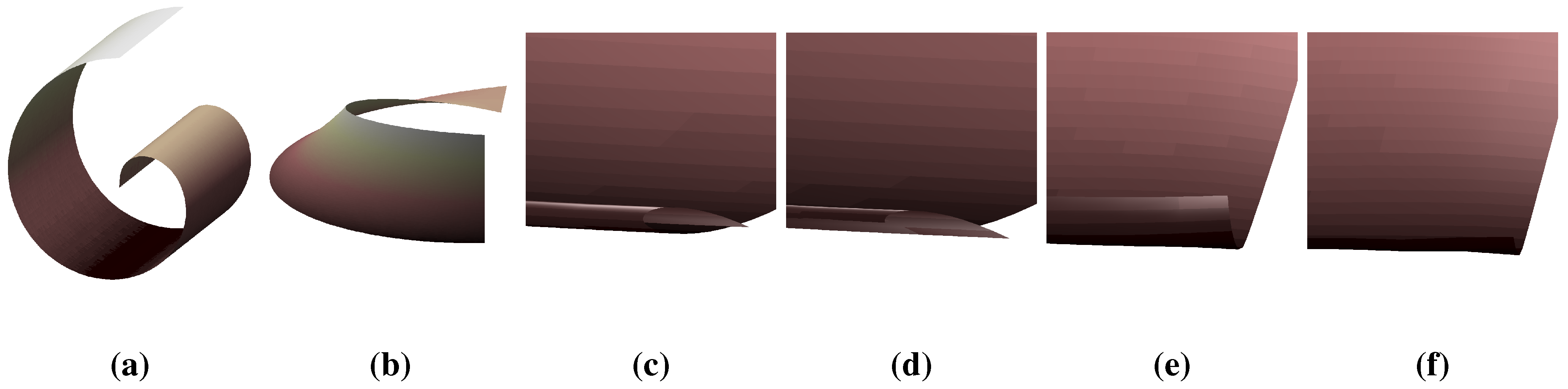
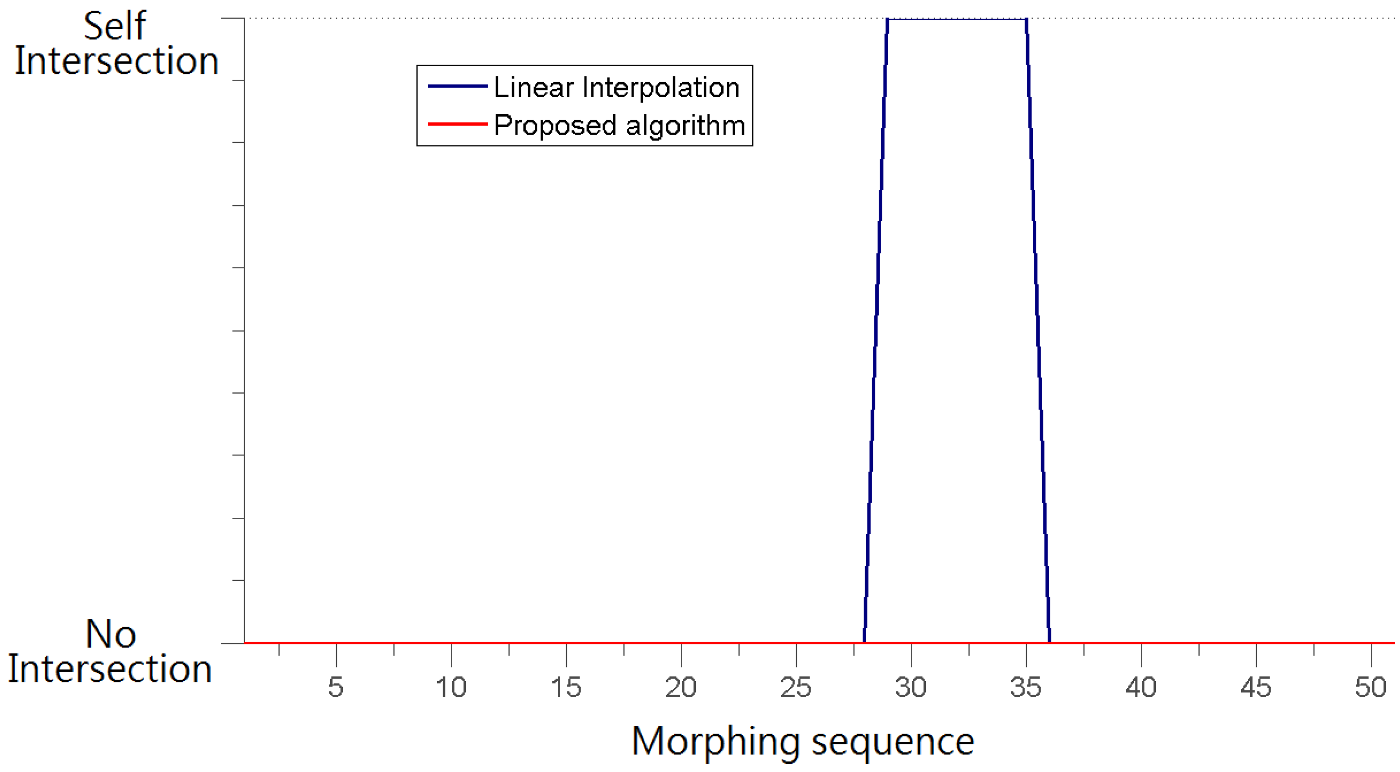
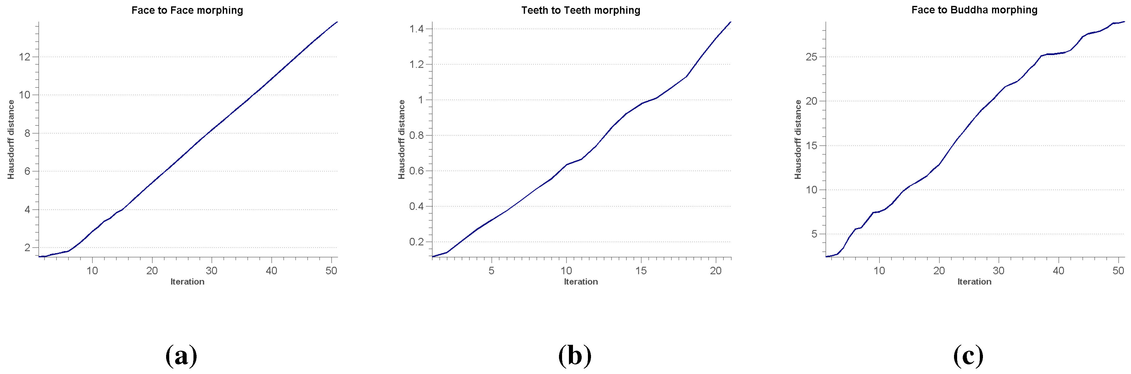
6.3. Surface Morphing

In the first experiment, we compare our method with the direct linear interpolation method. Figure 8a,b shows a spiral-generated surface and a partition of a Mobius strip surface, respectively, which are the original and the target surface of our morphing experiment. Figure 8c,d shows the 25th and 26th morphing sequence using linear interpolation, respectively. This example shows that an unnatural surface self-intersection may occur when morphing complicated surfaces with direct linear interpolation. Figure 8e,f shows the corresponding morphing sequence using our proposed algorithm. No self-intersection occurs in the morphing approximation. The occurrence of surface self-intersection using linear interpolation and our proposed algorithm is recorded in Figure 9.

Figure 8. Surface morphing between a spiral-generated surface and part of a Mobius strip. (a,b) The spiral-generated surface and Mobius strip part, respectively. (c,e) The 25th morphing sequence using linear interpolation and our proposed morphing algorithm, respectively. (d,f) The 26th morphing sequence using linear interpolation and our proposed morphing algorithm, respectively. The surface intersection occurs in the linear interpolation method.

Figure 8. Surface morphing between a spiral-generated surface and part of a Mobius strip. (a,b) The spiral-generated surface and Mobius strip part, respectively. (c,e) The 25th morphing sequence using linear interpolation and our proposed morphing algorithm, respectively. (d,f) The 26th morphing sequence using linear interpolation and our proposed morphing algorithm, respectively. The surface intersection occurs in the linear interpolation method.

Figure 9. Occurrence of surface self-intersection using linear interpolation and our proposed morphing algorithm. The plot shows the occurrence of surface self-intersection in morphing the spiral-generated surface to the part of the Mobius strip (see Figure 8a,b). Self-intersection occurs during the 29th–35th frames. Note also that no self-intersections appears when we apply our proposed morphing algorithm.

Figure 9. Occurrence of surface self-intersection using linear interpolation and our proposed morphing algorithm. The plot shows the occurrence of surface self-intersection in morphing the spiral-generated surface to the part of the Mobius strip (see Figure 8a,b). Self-intersection occurs during the 29th–35th frames. Note also that no self-intersections appears when we apply our proposed morphing algorithm.

We have tested our algorithm for morphing from one surface, $S_1$, to another, surface $S_2$, according to the $(\lambda ,H)$ representation. Figure 10 shows the synthetic human faces of a man (Figure 10a) and a woman (Figure 10f). We first obtain their corresponding $(\lambda ,H)$ representation, $({\lambda }_1,H_1)$ and $({\lambda }_2,H_2)$, and their boundary correspondence. Then, we approximate the surface evolution by linearly interpolating the $(\lambda ,H)$ representation between them. From this, we can get a sequence of pairs $\left(\lambda \right(t),H(t\left)\right)$, which approximate the morphing from surfaces $S_1$ to $S_2$. With these sequences of $(\lambda ,H)$ representation, we reconstruct the corresponding surfaces, as shown in Figure 10b–e. Experimental results show that the proposed algorithm can produce a natural morphing between different surfaces by simply interpolating the geometric quantities, λ and H, that can fully describe the surfaces.

Figure 10. Surface morphing between two human faces (from a male face to a female face) using the $(\lambda ,H)$ representations. (a,f) A male and a female face, respectively. By using the morphing algorithm, we interpolate λ and H and reconstruct the corresponding surface from the $(\lambda ,H)$ representation. (b–e) The morphing results.

Figure 10. Surface morphing between two human faces (from a male face to a female face) using the $(\lambda ,H)$ representations. (a,f) A male and a female face, respectively. By using the morphing algorithm, we interpolate λ and H and reconstruct the corresponding surface from the $(\lambda ,H)$ representation. (b–e) The morphing results.

We also test our morphing algorithm to interpolate between two teeth surfaces. Figure 11a,f shows the two human teeth surfaces. By using Algorithm 2, we interpolate λ and H and reconstruct the corresponding surfaces from the $(\lambda ,H)$ representation, as shown in Figure 11b–e. Figure 12 shows another example of morphing a human face to a partition of a Buddha surface. Figure 12a,f shows the original human face and the Buddha surface, respectively. With the proposed morphing algorithm, we first obtain the $(\lambda ,H)$ representations of the two surfaces. We again interpolate λ and H and reconstruct the morphing sequences, as shown in Figure 12b–e. Notice that by using the proposed algorithm, surface features, like local valleys and ridges, can naturally deform, as both are described by the mean curvature and conformal factor. Therefore, our proposed algorithm produces good morphing approximation, which follows the geometry of the two surfaces.

Figure 11. Surface morphing between two teeth using $(\lambda ,H)$ representation. (a,f) Tooth 1 and Tooth 2, respectively. By using the morphing algorithm, we interpolate λ and H and reconstruct the corresponding surface from the $(\lambda ,H)$ representation. (b–e) The morphing results. Note that a natural evolution of ridges and valleys from Tooth 1 to Tooth 2 is obtained.

Figure 11. Surface morphing between two teeth using $(\lambda ,H)$ representation. (a,f) Tooth 1 and Tooth 2, respectively. By using the morphing algorithm, we interpolate λ and H and reconstruct the corresponding surface from the $(\lambda ,H)$ representation. (b–e) The morphing results. Note that a natural evolution of ridges and valleys from Tooth 1 to Tooth 2 is obtained.

Figure 12. Surface morphing between a male face and a Buddha surface using $(\lambda ,H)$ representation. (a,f) The human face and the partition of a Buddha surface, respectively. By using the morphing algorithm, we interpolate λ and H and reconstruct the corresponding surface from the $(\lambda ,H)$ representation. (b–e) The morphing results.

Figure 12. Surface morphing between a male face and a Buddha surface using $(\lambda ,H)$ representation. (a,f) The human face and the partition of a Buddha surface, respectively. By using the morphing algorithm, we interpolate λ and H and reconstruct the corresponding surface from the $(\lambda ,H)$ representation. (b–e) The morphing results.

Figure 13 summaries the changes of the Hausdorff distance between the original surfaces and the corresponding morphing sequences of each example. Figure 13a–c shows the changes of the Hausdorff distance in the morphing results, as shown in Figure 10, Figure 11 and Figure 12, respectively. As shown in the figure, the Hausdorff distance increases monotonically during the morphing process. This assures that our algorithm gives a natural and smooth morphing result. To visualize the change of magnitude of the conformal factor, we obtain the harmonic parameterization of the morphing surfaces with the arc-length parameterized boundary condition from the original surface (see Figure 14). The color on the parameterized domains denotes the absolute value of the conformal factor from the corresponding morphing surfaces. Figure 14a–c corresponds to the parameterization of the 15th and 35th morphing surfaces from the morphing sequence results in Figure 10, Figure 11 and Figure 12, respectively.

Figure 13. Hausdorff distance between the morphing sequences of each example from their corresponding original surfaces. (a–c) The changes of the Hausdorff distance during the morphing examples, as shown in Figure 10 and Figure 11, respectively.

Figure 13. Hausdorff distance between the morphing sequences of each example from their corresponding original surfaces. (a–c) The changes of the Hausdorff distance during the morphing examples, as shown in Figure 10 and Figure 11, respectively.

Figure 14. Harmonic mapping of the morphing surfaces from the 15th and 35th frames with arc-length parameterized boundary conditions from the original surface. The color represents the conformal factor of the corresponding morphing surfaces. (a–c) The morphing examples, correspondingly as in Figure 10, Figure 11 and Figure 12, respectively.

Figure 14. Harmonic mapping of the morphing surfaces from the 15th and 35th frames with arc-length parameterized boundary conditions from the original surface. The color represents the conformal factor of the corresponding morphing surfaces. (a–c) The morphing examples, correspondingly as in Figure 10, Figure 11 and Figure 12, respectively.

7. Conclusions

This paper presents two novel algorithms for computing the multiscale representation of a surface and morphing between two surfaces. Instead of directly tackling the problems with the coordinate functions of the surfaces, we adopt the $(\lambda ,H)$ representation proposed earlier in [33,34]. By the Riemann surface theory, given any surface, S, we can find the conformal factor, λ, and mean curvature, H, which uniquely determine the surface, S. By using the $(\lambda ,H)$ representation, the problem of multi-scale representation is transformed to a signal processing problem of both geometric quantities λ and H. In other words, by treating the geometric quantities, λ and H, as signals, we can extract different scales of geometric detail from the surface through the surface reconstruction from the truncated $(\lambda ,H)$ representation.

Moreover, a surface morphing algorithm has also been proposed in this work. We consider to approximate the deformation of surfaces through their corresponding $(\lambda ,H)$ representations. To morph between two surfaces, we propose to linearly interpolate between the $(\lambda ,H)$ representations of the two surfaces. Since conformal factor and mean curvature can fully describe the geometric characteristics of the surface, our algorithm can effectively compute a natural morphing between two surfaces, as shown in the experimental results.

Note that our algorithms work on simply-connected open surfaces. In the future, we will consider extending our proposed algorithms on genus zero closed surfaces by making use of the spherical harmonic expansion and spherical harmonic conformal mapping. We will also consider extending our algorithms to point clouds.

References

1. Yuen, P.C. Multi-Scale Representation and Recognition of Three Dimensional Surfaces Using Geometric Invariants. Doctoral Dissertation, University of Surrey, Guildford, UK, 2001. [Google Scholar]
2. Pauly, M.; Keiser, R.; Gross, M. Multi-scale Feature Extraction on Point Sampled Surfaces. Comput. Graph. Forum 2003, 22, 281–289. [Google Scholar] [CrossRef]
3. Fadaifard, H.; Wolberg, G. Multiscale 3D feature extraction and matching. In Proceedings of the 3D Imaging, Modeling, Processing, Visualization and Transmission (3DIMPVT), Hangzhou, China, 16–19 May 2011; pp. 228–235.
4. Vaillant, M.; Glaunes, J. Surface matching via currents. In Information Processing in Medical Imaging; Springer: New York, NY, USA, 2005; pp. 381–392. [Google Scholar]
5. Yeo, B.T.; Sabuncu, M.R.; Vercauteren, T.; Ayache, N.; Fischl, B.; Golland, P. Spherical demons: Fast diffeomorphic landmark-free surface registration. IEEE Trans. Med. Imaging 2010, 29, 650–668. [Google Scholar] [CrossRef] [PubMed]
6. Granger, S.; Pennec, X. Multi-scale EM-ICP: A fast and robust approach for surface registration. Lect. Notes Comput. Sci. 2002, 2353, 418–432. [Google Scholar]
7. Risser, L.; Vialard, F.; Wolz, R.; Murgasova, M.; Holm, D.D.; Rueckert, D. Simultaneous multi-scale registration using large deformation diffeomorphic metric mapping. IEEE Trans. Med. Imaging 2011, 30, 1746–1759. [Google Scholar] [CrossRef] [PubMed]
8. Kircher, S.; Garland, M. Editing arbitrarily deforming surface animations. ACM Trans. Graph. (TOG) 2006, 25, 1098–1107. [Google Scholar] [CrossRef]
9. Gu, X.; Wang, Y.; Chan, T.F.; Thompson, P.M.; Yau, S.T. Genus zero surface conformal mapping and its application to brain surface mapping. In Information Processing in Medical Imaging; Springer: Berlin/Heidelberg, Germany, 2003; pp. 172–184. [Google Scholar]
10. Wang, Y.; Lui, L.M.; Gu, X.; Hayashi, K.M.; Chan, T.F.; Toga, A.W.; Yau, S.T. Brain surface conformal parameterization using Riemann surface structure. IEEE Trans. Med. Imaging 2007, 26, 853–865. [Google Scholar] [CrossRef] [PubMed]
11. Gu, X.; Yau, S.T. Computing conformal structure of surfaces. Communications in Information and Systems 2002, 2, 121–146. [Google Scholar] [CrossRef]
12. Fischl, B.; Sereno, M.I.; Tootell, R.B.; Dale, A.M. High-resolution intersubject averaging and a coordinate system for the cortical surface. Human brain mapping 1999, 8, 272–284. [Google Scholar] [CrossRef]
13. Haker, S.; Angenent, S.; Tannenbaum, A.; Kikinis, R.; Sapiro, G.; Halle, M. Conformal surface parameterization for texture mapping. IEEE Trans. Vis. Comput. Graph. 2000, 6, 181–189. [Google Scholar] [CrossRef]
14. Hurdal, M.K.; Stephenson, K. Discrete conformal methods for cortical brain flattening. Neuroimage 2009, 45, S86–S98. [Google Scholar] [CrossRef] [PubMed]
15. Lévy, B.; Petitjean, S.; Ray, N.; Maillot, J. Least squares conformal maps for automatic texture atlas generation. ACM Trans. Graph. 2002, 21, 362–371. [Google Scholar] [CrossRef]
16. Desbrun, M.; Meyer, M.; Alliez, P. Intrinsic parameterizations of surface meshes. In Proceedings of the Eurographics, Saarbruecken, Germany, 2–6 September, 2002; pp. 209–218.
17. Lui, L.M.; Wong, T.W.; Zeng, W.; Gu, X.; Thompson, P.M.; Chan, T.F.; Yau, S.T. Optimization of surface registrations using beltrami holomorphic flow. J. Sci. Comput. 2012, 50, 557–585. [Google Scholar] [CrossRef]
18. Lui, L.M.; Wong, T.W.; Thompson, P.; Chan, T.; Gu, X.; Yau, S.T. Shape-based diffeomorphic registration on hippocampal surfaces using beltrami holomorphic flow. In Proceedings of the Medical Image Computing and Computer-Assisted Intervention MICCAI, Beijing, China, 20–24 September, 2010; pp. 323–330.
19. Khodakovsky, A.; Schroder, P.; Sweldens, W. Progressive geometry compression. In Proceedings of the 27th Annual Conference on Computer Graphics and Interactive Techniques, New Orleans, LA, USA, 23–28 July, 2000; pp. 271–278.
20. Peyré, G.; Mallat, S. Surface compression with geometric bandelets. ACM Trans. Graph. (TOG) 2005, 24, 601–608. [Google Scholar] [CrossRef]
21. Eck, M.; DeRose, T.; Duchamp, T.; Hoppe, H.; Lounsbery, M.; Stuetzle, W. Multiresolution analysis of arbitrary meshes. In Proceedings of the 22nd Annual Conference on Computer Graphics and Interactive Techniques, Los Angeles, CA, USA, 6–11 August, 1995; pp. 173–182.
22. Gross, M.H.; Hubeli, A. Eigenmeshes. Technical Report. Department of Computer Science, ETH Zurich: Zurich, Switzerland, 2000. [Google Scholar]
23. Cipriano, G.; Phillips, G.N.; Gleicher, M. Multi-scale surface descriptors. IEEE Trans. Vis. Comput. Graph. 2009, 15, 1201–1208. [Google Scholar] [CrossRef] [PubMed]
24. Ho, H.T.; Gibbins, D. Multi-scale feature extraction for 3D surface registration using local shape variation. In Proceedings of the IEEE 23rd International Conference Image and Vision Computing New Zealand, IVCNZ 2008, Christchurch, New Zealand, 26–28 November, 2008; pp. 1–6.
25. Pauly, M.; Kobbelt, L.P.; Gross, M. Point-based multiscale surface representation. ACM Trans. Graph. (TOG) 2006, 25, 177–193. [Google Scholar] [CrossRef]
26. Liu, Y.S.; Yan, H.B.; Martin, R.R. As-Rigid-As-Possible Surface Morphing. J. Comput. Sci. Technol. 2011, 26, 548–557. [Google Scholar] [CrossRef]
27. Alexa, M.; Cohen-Or, D.; Levin, D. As-rigid-as-possible shape interpolation. In Proceedings of the 27th Annual Conference on Computer Graphics and Interactive Techniques, New Orleans, LA, USA, 23–28 July, 2000; pp. 157–164.
28. Kanai, T.; Suzuki, H.; Kimura, F. Three-dimensional geometric metamorphosis based on harmonic maps. Vis. Comput. 1998, 14, 166–176. [Google Scholar] [CrossRef]
29. Hojjat, M.; Stavropoulou, E.; Bletzinger, K.U. The vertex morphing method for node-based shape optimization. Comput. Methods Appl. Mech. Eng. 2014, 268, 494–513. [Google Scholar] [CrossRef]
30. Rajamani, K.T.; Ballester, M.A.G.; Nolte, L.P.; Styner, M. A novel and stable approach to anatomical structure morphing for enhanced intraoperative 3D visualization. Medical Imaging 2005, 718–725, Proc. SPIE 2005, 5744, 718–725. [Google Scholar]
31. Hughes, J.F. Scheduled Fourier volume morphing. In Proceedings of the ACM SIGGRAPH Computer Graphics, Chicago, IL, 27–31 July, 1992; Volume 26, pp. 43–46.
32. Turk, G.; O’Brien, J.F. Shape transformation using variational implicit functions. In Proceedings of the ACM SIGGRAPH 2005 Courses, New York, NY, USA, 2–4, August, 2005. [CrossRef]
33. Gu, X.; Wang, Y.; Yau, S.T. Geometric compression using Riemann surface structure. Commun. Inf. Syst. 2004, 2, 171–182. [Google Scholar] [CrossRef]
34. Lui, L.M.; Wen, C.; Gu, X. A Conformal Approach for Surface Inpainting. AIM Inverse Problems Imaging 2013, 7, 863–884. [Google Scholar]
35. Gruen, A.; Akca, D. Least squares 3D surface and curve matching. ISPRS J. Photogramm. Remote Sens. 2005, 59, 151–174. [Google Scholar] [CrossRef]
36. Lui, L.M.; Lam, K.C.; Wong, T.W.; Gu, X. Texture map and video compression using Beltrami representation. SIAM J. Imaging Sci. 2013, 6, 1880–1902. [Google Scholar] [CrossRef]