The Generalized Schur Algorithm and Some Applications


1
Istituto per le Applicazioni del Calcolo “M. Picone”, CNR, Sede di Bari, via G. Amendola 122/D, 70126 Bari, Italy
2
Catholic University of Louvain, Department of Mathematical Engineering, Avenue Georges Lemaitre 4, B-1348 Louvain-la-Neuve, Belgium
*
Author to whom correspondence should be addressed.
Axioms 2018, 7(4), 81; https://doi.org/10.3390/axioms7040081
Submission received: 2 October 2018
/
Revised: 5 November 2018
/
Accepted: 7 November 2018
/
Published: 9 November 2018
(This article belongs to the Special Issue Advanced Numerical Methods in Applied Sciences)
Abstract
:The generalized Schur algorithm is a powerful tool allowing to compute classical decompositions of matrices, such as the and factorizations. When applied to matrices with particular structures, the generalized Schur algorithm computes these factorizations with a complexity of one order of magnitude less than that of classical algorithms based on Householder or elementary transformations. In this manuscript, we describe the main features of the generalized Schur algorithm. We show that it helps to prove some theoretical properties of the R factor of the factorization of some structured matrices, such as symmetric positive definite Toeplitz and Sylvester matrices, that can hardly be proven using classical linear algebra tools. Moreover, we propose a fast implementation of the generalized Schur algorithm for computing the rank of Sylvester matrices, arising in a number of applications. Finally, we propose a generalized Schur based algorithm for computing the null-space of polynomial matrices.
1. Introduction
The generalized Schur algorithm (GSA) allows computing well-known matrix decompositions, such as and factorizations [1]. In particular, if the involved matrix is structured, i.e., Toeplitz, block-Toeplitz or Sylvester, the GSA computes the R factor of the factorization with complexity of one order of magnitude less than that of the classical algorithm [2], since it relies only on the knowledge of the so-called generators [2] associated to the given matrix, rather than on the knowledge of the matrix itself. The stability properties of the GSA are described in [3,4,5], where it is proven that the algorithm is weakly stable provided the involved hyperbolic rotations are performed in a stable way.
In this manuscript, we first show that, besides the efficiency properties, the GSA provides new theoretical insights on the bounds of the entries of the R factor of the factorization of some structured matrices. In particular, if the involved matrix is a symmetric positive definite (SPD) Toeplitz or a Sylvester matrix, we prove that all or some of the diagonal entries of R monotonically decrease in absolute value.
We then propose a faster implementation of the algorithm described in [6] for computing the rank of a Sylvester matrix whose entries are the coefficients of two polynomials of degree m and n, respectively. This new algorithm is based on the GSA for computing the R factor of the factorization of The proposed modification of the GSA-based method has a computational cost of floating point operations, where and r is the computed numerical rank.
It is well known that the upper triangular factor R factor of the factorization of a matrix is equal to the upper triangular Cholesky factor of up to a diagonal sign matrix D, i.e., In this manuscript, we assume, without loss of generality, that the diagonal entries of R and are positive and since the matrices are then equal, we denote both matrices by R.
Finally, we propose a GSA-based approach for computing a null-space basis of a polynomial matrix, which is an important problem in several systems and control applications [7,8]. For instance, the computation of the null-space of a polynomial matrix arises when solving the column reduction problem of a polynomial matrix [9,10].
The manuscript is structured as follows. The main features of the GSA are provided in Section 2. In Section 3, a GSA implementation for computing the Cholesky factor R of a SPD Toeplitz matrix is described, which allows proving that the diagonal entries of R monotonically decrease. In Section 4, a GSA-based algorithm for computing the rank of a Sylvester matrix S is introduced, based on the computation of the Cholesky factor R of In addition, in this case, it is proven that the first diagonal entries of R monotonically decrease. The GSA-based method to compute the null-space of polynomial matrices is proposed in Section 5. The numerical examples are reported in Section 6 followed by the conclusions in Section 7.
2. The Generalized Schur Algorithm
Many of the classical factorizations of a symmetric matrix, e.g., and can be obtained by the GSA. If the matrix is Toeplitz-like, the GSA computes these factorizations in a fast way. For the sake of completeness, the basic concepts of the GSA for computing the R factor of the factorization of structured matrices, such as Toeplitz and block-Toeplitz matrices, are introduced in this Section. A comprehensive treatment of the topic can be found in [1,2].
Let be a symmetric positive definite (SPD) matrix. The semidefinite case is considered in Section 4 and Section 5. The displacement of A with respect to a matrix Z of order is defined as
while the displacement rank k of A with respect to Z is defined as the rank of If Equation (1) can be written as the sum of k rank-one matrices,
where is the inertia of and the vectors are called the positive and the negative generators of A with respect to respectively, conversely, if there is no ambiguity, simply the positive and negative generators of A. The matrix is called the generator matrix.
The matrix Z is a nilpotent matrix. In particular, for Toeplitz and block-Toeplitz matrices, the matrix Z can be chosen as the shift and the block shift matrix
respectively.
The implementation of the GSA relies only on the knowledge of the generators of A rather than on the knowledge of the matrix itself [1].
Let
Since
then, adding all members of the left and right-hand sides of Equation (2) yields
which expresses the matrix A in terms of its generators.
Exploiting Equation (2), we show how the GSA computes R by describing its first iteration. Observe that the matrix products involved in the right-hand side of Equation (2) have their first row equal to zero, with the exception of the first product, .
Any such matrix can be constructed in different ways [11,12,13,14]. For instance, it can be considered as the product of Givens and hyperbolic rotations. In particular, a Givens rotation acting on rows i and j of the generator matrix is chosen if Otherwise, a hyperbolic rotation is considered. Indeed, suitable choices of allow efficient implementations of GSA, as shown in Section 4.
Let and be a J-orthogonal matrix such that
and be the ith column of the identity matrix. Furthermore, let and be the first and last rows of respectively, i.e.,
From Equation (4), it turns out that the first column of is zero. Let be the matrix obtained by deleting the first row and column from J. Then, Equation (2) can be written as follows,
where that is, is obtained from by multiplying with and If A is a Toeplitz matrix, this multiplication with Z corresponds to displacing the entries of one position downward, while it corresponds to a block-displacement downward in the first generator if A is a block-Toeplitz matrix.
Thus, the first column of is zero and, hence, is the first row of the R factor of the factorization of The above procedure is recursively applied to to compute the other rows of
The jth iteration of GSA, involves the products and . The former multiplication can be computed in operations [11,12], and the latter is done for free if Z is either a shift or a block–shift matrix. Therefore, if the displacement rank k of A is small compared to the GSA computes the R factor in rather than in operations, as required by standard algorithms [15].
For the sake of completeness, the described GSA implementation is reported in the following matlab style function. (The function givens is the matlab function having as input two scalars, and and as output an orthogonal matrix such that The function Hrotate computes the coefficients of the hyperbolic rotation such that, given two scalars and The function Happly applies to two rows of the generator matrix. Both functions are defined in [12]).
functionGSA
fori = 1 : n,
for j = 2 : k1,
givens
end % for
for j = k1 + 2 : k1 + k2,
Θ = govens(G(k1 + 1, i), G(j, i));
G([k1 + 1, j], i : n) = Θ ∗ G[k1 + 1, j], i : n);
end % for
[c1, s1] = Hrotate(G(1, i), G(k1 + 1, i));
G([1, k1 + 1], i : n) = Happly(c1, s1, G([1, k1 + 1], i : n), n − i + 1);
R(i, i : n) = G(1, i : n);
G(1, i + 1 : n) = G(1, i : n − 1); G(1, i) = 0;
end % for
3. GSA for SPD Toeplitz Matrices
In this section, we describe the GSA for computing the R factor of the Cholesky factorization of a SPD Toeplitz matrix A, with R upper triangular, i.e., Moreover, we show that the diagonal entries of R decrease monotonically.
Let and be a SPD Toeplitz matrix and a shift matrix, respectively, i.e.,
and let Then,
i.e., is a symmetric rank-2 matrix. Moreover, the generator matrix G is given by
In this case, the GSA can be implemented in matlab-like style as follows.
functionGSA_chol
fori = 1 : n,
[c1, s1] = Hrotate(Gi − 1(1, i), G(i)(2, i)); Gi − 1(:, i : n) = Happly(c1, s1, Gi − 1(:, i : n), n − i + 1);
R(i, i : n) = Gi − 1(1, i : n);
Gi(1, i + 1 : n) = Gi − 1(1, i : n − 1); Gi(2, i + 1 : n) = Gi − 1(2, i + 1 : n − 1);
end % for
The following lemma holds.
Lemma 1.
Let A be a SPD Toeplitz matrix and let R be its Cholesky factor, with R upper triangular. Then,
Proof.
At each step i of GSA_chol, first a hyperbolic rotation is applied to in order to annihilate the element Hence, the first row of becomes the row i of Finally, is obtained displacing the entries of the first row of one position right, while is equal to Taking into account that the diagonal entries of R are
□
4. Computing the Rank of Sylvester Matrices
In this section, we focus on the computation of the rank of Sylvester matrices. The numerical rank of a Sylvester matrix is a useful information for determining the degree of the greatest common divisor of the involved polynomials [6,16,17].
A GSA-based algorithm for computing the rank of S has been recently proposed in [6]. It is based on the computation of the Cholesky factor R of with R upper triangular, i.e.,
Here, we propose a more efficient variant of this algorithm that allows proving that the first entries of R monotonically decrease.
Let and let Denote by and two univariate polynomials,
Let be the Sylvester matrix defined as follows,
with and band Toeplitz matrices.
We now describe how the GSA-based algorithm proposed in [6] for computing the rank of S can be implemented in a faster way. This variant is based on the computation of the Cholesky factor of with R upper triangular, i.e.,
Defining
the generator matrix G of with respect to Z is then given by [6]
where
with the jth vector of the canonical basis of and .
The algorithm proposed in [6] is based on the following GSA implementation for computing the R factor of the factorization of
functionGSA_chol2
fori = 1 : n,
Θ1 = givens(G(1, i), G(2, i)); Θ2 = givens(G(3, i), G(4, i));
G(1 : 2, i : n) = Θ1G(1 : 2, i : n); G(3 : 4, i : n) = Θ2G(3 : 4, i : n);
[c1, s1] = Hrotate(G(1, i), G(3, i));
G([1,3], i : n) = Happly(c1, s1, G([1,3], i : n), n − i + 1);
R(i, i : n) = Gi(1, i : n);
G(1, i + 1 : n) = G(1, i : n − 1)ZT; G(2, i + 1 : n) = G(2 : 4, i + 1 : n − 1);
end % for
At the ith iteration of the algorithm, the Givens rotations and are computed and applied, respectively, to the first and second generators, and to the third and fourth generators, to annihilate and Hence, the hyperbolic rotation is applied to the first and the third row of G to annihilate Finally, the first row of G becomes the ith row of R and the first row of G is multiplied by
Summarizing, at the first step of the ith iteration of GSA, all entries of the ith column but the first one of G, are annihilated. If the number of rows of G is greater than this can be accomplished in different ways (see [5,14]).
Analyzing the pattern of the generators in Equation (8), we are able to derive a different implementation of that costs , with . Moreover, this implementation allows proving that the first l diagonal entries of R are monotonically decreasing.
Since
if from Equation (9), it turns out that Moreover, the rows and have their first entry equal to zero and differ only in their entry in column This particular pattern of G is close to the ones described in [13,14,18], allowing to design an alternative GSA implementation with respect to that considered in [6], and thereby reducing the complexity from to , where r is the computed rank of S and
Since the description of the above GSA implementation is quite cumbersome and similar to the algorithms reported in [13,14,18], we omit it here. The corresponding matlab pseudo–code can be obtained from the authors upon request.
If the matrix S has rank at the st iteration, it turns out that in exact arithmetic [6]. Therefore, at each iteration of the algorithm we check whether
where is a fixed tolerance. If Equation (10) is not satisfied, we stop the computation considering k as the computed numerical rank of
The R factor of the factorization of S is unique if the diagonal entries of R are positive. The considered GSA implementation, yielding the rank of S and based on computing the R factor of the factorization of S, allows us to prove that the first l entries of the diagonal of R are ordered in a decreasing order, with In fact, the following theorem holds.
Theorem 1.
Let be the Cholesky factorization of with S the Sylvester matrix defined in Equation (6) with rank Then,
Proof.
Each entry i of the diagonal of R is determined by the ith entry of the first row of G at the end of iteration for Let us define and consider the following alternative implementation of the GSA for computing the first l columns of the Cholesky factor of
for
givens
Hrotate
Hrotate
end % for
We observe that, for , is the only entry in the first column of different from Hence, and the first iteration amounts only to shifting one position rightward, i.e.,
At the beginning of iteration the second and the fourth row of are equal Equation (8). Hence, when applying a Givens rotation to the first and the second row in order to annihilate the entry and when subsequently applying a hyperbolic rotation to the first and fourth row of in order to annihilate it turns out that and are then modified but still equal to each other, while remains unchanged. The equality between and is maintained throughout the iterations
Therefore, the second and the fourth row of do not play any role in computing and can be neglected. Hence, the GSA for computing reduces only to applying a hyperbolic rotation to the first and the third generators, as described in the following algorithm.
for
Hrotate
end % for
Since at the beginning of iteration then the involved hyperbolic rotation is such that
where the updated is equal to Therefore, and thus □
Remark 1.
The above GSA implementation allows to prove the inequality Equation (11). This property is difficult to obtain if the factorization is performed via Householder transformations or if the classical Cholesky factorization of is used.
5. GSA for Computing the Null-Space of Polynomial Matrices
In this section, we consider the problem of computing a polynomial basis of the null-space of an polynomial matrix of degree and rank
As described in [8,19,20], the above problem is equivalent to that of computing the null-space of a related block-Toeplitz matrix. Algorithms to solve this problem are proposed in [8,19] but they do not explicitly exploit the structure of the involved matrix. Algorithms to solve related problems have also been described in the literature, e.g., in [8,19,21,22].
In this paper, we propose an algorithm for computing the null-space of polynomial matrices based on a variant of the GSA for computing the null-space of a related band block-Toeplitz matrix [8].
5.1. Null-Space of Polynomial Matrices
A polynomial vector is said to belong to the null-space of (12) if
The polynomial vector belongs to the null-space of iff is a vector belonging to the null-space of the band block-Toeplitz matrix
where with the number of block columns of that can be determined, e.g., by the algorithm described in [8]. Hence, the problem of computing the null-space of the polynomial matrix in Equation (12) is equivalent to the problem of computing the null-space of the matrix in Equation (13). To normalize the entries in this matrix, it is appropriate to first perform a QR factorization of each block column of T:
and to absorb the upper triangular factor U in the vector . The convolution equation then becomes an equation of the type but where the coefficient matrices of form together an orthonormalized matrix.
Remark 2.
Above, we have assumed that there are no constant vectors in the kernel of . If there are, then, the block column of matrices has rank less than n and the above factorization will discover it in the sense that the matrix U is nonsquare and the matrices have less columns than This trivial null-space can be eliminated and we therefore assume that the rank was full. For simplicity, from now on, we also assume that the coefficient matrices of the polynomial matrix were already normalized in this way and the norm of the block columns of T are thus orthonormalized. This normalization proves to be very useful in the sequel.
Denote by
where is the null–matrix of order
If and i.e.,
and then also In this case, the vector is said to be a generator vector of a chain of length of the null-space of
The proposed algorithm for the computation of the null-space of polynomial matrices is based on the GSA for computing the R factor of the -factorization of the matrix T in Equation (13) and, if R is full column rank, its inverse .
Let us first assume that the matrix T is full rank, i.e., Without loss of generality, we suppose If the algorithm still computes the R factor in trapezoidal form [23]. Moreover, in this case, we compute the first rows of the inverse of the matrix obtained appending the last rows of the identity matrix of order to
Let us consider the SPD block-Toeplitz matrix
whose blocks are
Notice that, because of the normalization introduced before, we have that and . This is used below. The matrix
can be factorized in the following way,
where is the factor R of the -factorization of i.e., the Cholesky factor of Hence, R and its inverse can be retrieved from the first columns of the matrix
The displacement matrix and the displacement rank of W with respect to are given by
and respectively, with
Then, taking the order n of the matrices into account, it turns out that
Since the construction of G does not require any computation: it is easy to check that G is given by
Remark 3.
Observe that increasing with the structures of W and do not change due to the block band structure of the matrix W. Consequently, the length of the corresponding generators changes but their structure remains the same since only and are different from zero in the first block row.
The computation by the GSA of the R factor of T and of its inverse is made by only using the matrix G rather than the matrix T. Its implementation is a straightforward block matrix extension of the GSA described in Section 2.
Remark 4.
By construction, the initial generator matrix has the first block rows and the block row different from zero. Therefore, the multiplication of by the J-orthogonal matrix does not modify the structure of the generator matrix.
Let At each iteration i (for ), we start from the generator matrix having the blocks (of length n) and different form zero. We then look for a J-orthogonal matrix such that the product has in position and a nonsingular upper triangular and zero matrix, respectively.
Then, is obtained from by multiplying the first n columns with i.e.,
The computation of the J-orthogonal matrix at the ith iteration of the GSA can be constructed as a product of n Householder matrices and n hyperbolic rotations
The multiplication by the Householder matrices modifies the last n columns of the generator matrix, annihilating the last n entries but the st in the row while the multiplication by the hyperbolic rotations acts on the columns i and annihilating the entry in position
Given a hyperbolic matrix can be computed
such that
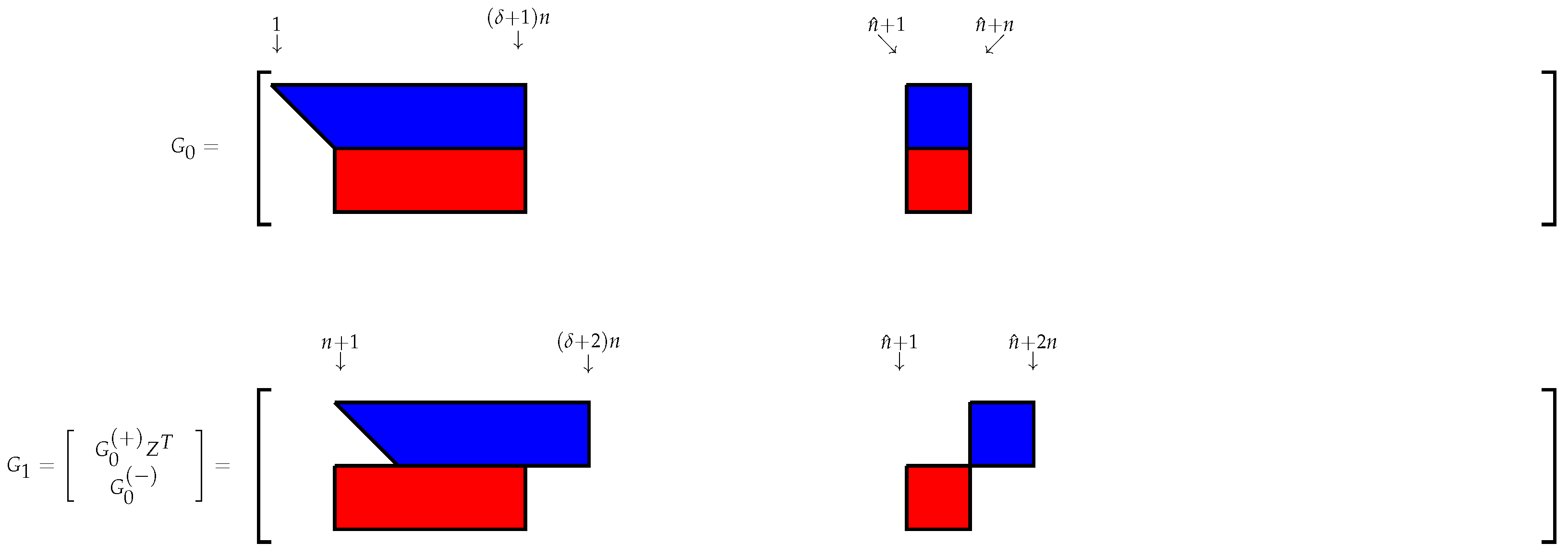
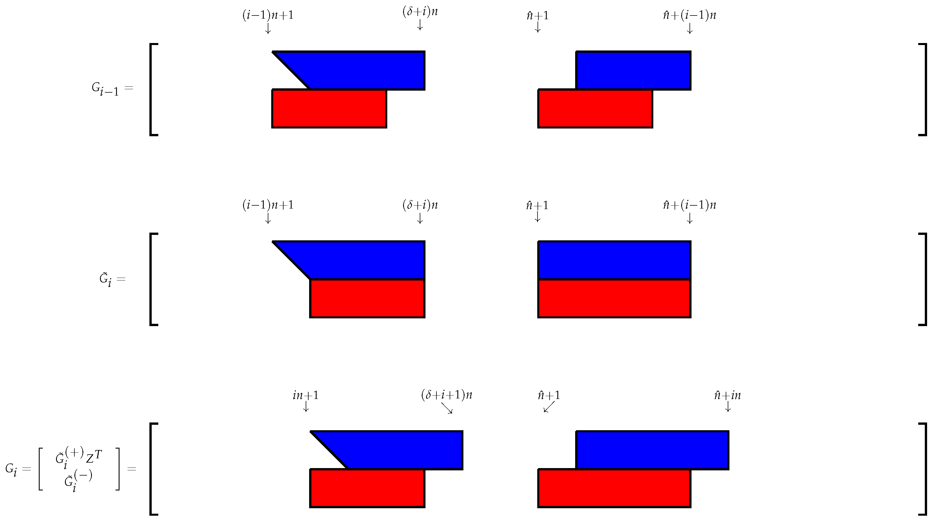
The modification of the sparsity pattern of the generator matrix after the first and ith iteration of the GSA are displayed in Figure 1 and Figure 2, respectively.
The reliability of the GSA strongly depends on the way the hyperbolic rotation is computed. In [4,5,24], it is proven that the GSA is weakly stable if the hyperbolic rotations are implemented in an appropriate manner [3,11,12,24].
Let
Then,
As previously mentioned, GSA relies only on the knowledge of the generators of W rather than on the matrix itself. Its computation involves the product which can be accomplished with flops. The ith iteration of the GSA involves the multiplication of n Householder matrices of size n times a matrix of size Therefore, since the cost of the multiplication by the hyperbolic rotation is negligible with respect to that of the multiplication by the Householder matrices, the computational cost at iteration i is . Hence, the computational cost of GSA is .
5.2. GSA for Computing the Right Null-Space of Semidefinite Block Toeplitz Matrices
As already mentioned in Section 5.1, the number of desired blocks of the matrix T in Equation (13) can be computed as described in [8]. For the sake of simplicity, in the considered examples, we choose large enough to compute the null-space of
The structure and the computation via the GSA of the R factor of the factorization of the singular block Toeplitz matrix T with rank is considered in [23].
A modification of the GSA for computing the null-space of Toeplitz matrices is described in [25]. In this paper, we extend the latter results to compute the null-space of T by modifying GSA.
Without loss of generality, let us assume that the first columns of T are linear independent and suppose that the th column linearly depends on the previous ones. Therefore, the first principal minors of are positive while the th one is zero. Let be the spectral decomposition of with orthogonal and with
and let with with Hence,
Let be the Cholesky factor of with upper triangular, i.e., Then,
On the other hand,
where Hence, as the last column of becomes closer and closer to a multiple of the eigenvector corresponding to the 0 eigenvalue of
Therefore, given
we have that
Let
Define
Hence,
We observe that column of the generator matrix is not involved in the GSA until the very last iteration, since only its th entry is different from At the very last iteration, the hyperbolic rotation
with
is applied to the th and st rows of i.e., to the nth row of and the first one of . Since is singular, it turns out that (see [23,25]). Thus,
where
We observe that, as
Since a vector of the right null-space of T is determined except for the multiplication by a constant, neglecting the term such a vector can be computed at the last iteration as the first column of the product
When detecting a vector of the null-space as a linear combination of row n of and row one of the new generator matrix G for the GSA is obtained removing the latter columns from G [23,25].
The implementation of the modified GSA for computing the null-space of band block-Toeplitz matrices in Equation (13) is rather technical and can be obtained from the authors upon request.
6. Numerical Examples
All the numerical experiments were carried out in matlab with machine precision . Example 1 concerns the computation of the rank of a Sylvester matrix, while Examples 2 and 3 concern the computation of the null-space of polynomial matrices.
Example 1.
Let and be random numbers generated by thematlabfunctionrandn. Let and be the two polynomials of degree 15 and 18, constructed by the matlab functionpoly, whose roots are, respectively, and and and
The greatest common divisor of w and y has degree 3 and, therefore, the Sylvester matrix constructed from anf has rank The diagonal entries of the R factor computed by the implementation described in Section 4 are displayed in Figure 3. Observe that the rank of the matrix can be retrieved by the number of entries of R above a certain tolerance. Moreover, it can be noticed that the first diagonal entries monotonically decrease.
Example 2.
As second example, we consider the computation of the coprime factorization of a transfer function matrix, described in [9,26]. The results obtained by the proposed GSA-based algorithm were compared with those obtained computing the null-space of the considered matrix by the functionsvdofmatlab.
Let be the transfer function with
Let
Let us consider Then, is the block-Toeplitz matrix constructed from as described in Section 5.1. Let and be the rank and the singular value decomposition of T computed bymatlab, respectively, and let us define and the matrices of the right singular vectors corresponding to the nonzero and zero singular values of respectively. The modified GSA applied to T yields four vectors belonging to the right null-space of with Let In Table 1, the relative norm of , the relative norm of , the norm of and the norm of are reported in Columns 1–4, respectively.
Such values show that the results provided bysvdofmatlaband by the algorithm based on a modification of GSA are comparable in terms of accuracy.
Example 3.
Let A right coprime pair for is given by
Let us choose Then, is the block-Toeplitz matrix constructed from as described in Section 5.1. Let and be the rank and the singular value decomposition of T computed bymatlab, respectively, and let define and the matrices of the right singular vectors corresponding to the nonzero and zero singular values of respectively. The modified GSA applied to T yields the vectors of the right null-space, with Let In Table 2, the relative norm of , the relative norm of , the norm of and the norm of are reported in Columns 1–4, respectively.
As in Example 2, the results yielded by the considered algorithms are comparable in accuracy.
7. Conclusions
The Generalized Schur Algorithm is a powerful tool allowing to compute classical decompositions of matrices, such as the and factorizations. If the involved matrices have a particular structure, such as Toeplitz or Sylvester, the GSA computes the latter factorizations with a complexity of one order of magnitude less than that of classical algorithms based on Householder or elementary transformations.
After having emphasized the main features of the GSA, we have shown in this manuscript that the GSA helps to prove some theoretical properties of the R factor of the factorization of some structured matrices. Moreover, a fast implementation of the GSA for computing the rank of Sylvester matrices and the null-space of polynomial matrices is proposed, which relies on a modification of the GSA for computing the R factor and its inverse of the factorization of band block-Toeplitz matrices with full column rank. The numerical examples show that the proposed approach yields reliable results comparable to those ones provided by the function svd of matlab.
Author Contributions
All authors contributed equally to this work.
Funding
This research was partly funded by INdAM-GNCS and by CNR under the Short Term Mobility Program.
Conflicts of Interest
The authors declare no conflict of interest.
References
- Kailath, T.; Sayed, A.H. Fast Reliable Algorithms for Matrices with Structure; SIAM: Philadelphia, PA, USA, 1999. [Google Scholar]
- Kailath, T.; Sayed, A. Displacement Structure: Theory and Applications. SIAM Rev. 1995, 32, 297–386. [Google Scholar] [CrossRef]
- Chandrasekaran, S.; Sayed, A. Stabilizing the Generalized Schur Algorithm. SIAM J. Matrix Anal. Appl. 1996, 17, 950–983. [Google Scholar] [CrossRef]
- Stewart, M.; Van Dooren, P. Stability issues in the factorization of structured matrices. SIAM J. Matrix Anal. Appl. 1997, 18, 104–118. [Google Scholar] [CrossRef]
- Mastronardi, N.; Van Dooren, P.; Van Huffel, S. On the stability of the generalized Schur algorithm. Lect. Notes Comput. Sci. 2001, 1988, 560–567. [Google Scholar]
- Li, B.; Liu, Z.; Zhi, L. A structured rank-revealing method for Sylvester matrix. J. Comput. Appl. Math. 2008, 213, 212–223. [Google Scholar] [CrossRef]
- Forney, G. Minimal bases of rational vector spaces with applications to multivariable linear systems. SIAM J. Control Optim. 1975, 13, 493–520. [Google Scholar] [CrossRef]
- Zúñiga Anaya, J.; Henrion, D. An improved Toeplitz algorithm for polynomial matrix null-space computation. Appl. Math. Comput. 2009, 207, 256–272. [Google Scholar] [CrossRef] [Green Version]
- Beelen, T.; van der Hurk, G.; Praagman, C. A new method for computing a column reduced polynomial matrix. Syst. Control Lett. 1988, 10, 217–224. [Google Scholar] [CrossRef] [Green Version]
- Neven, W.; Praagman, C. Column reduction of polynomial matrices. Linear Algebra Its Appl. 1993, 188, 569–589. [Google Scholar] [CrossRef]
- Bojańczyk, A.; Brent, R.; Van Dooren, P.; de Hoog, F. A note on downdating the Cholesky factorization. SIAM J. Sci. Stat. Comput. 1987, 8, 210–221. [Google Scholar] [CrossRef]
- Higham, N.J. J-orthogonal matrices: properties and generation. SIAM Rev. 2003, 45, 504–519. [Google Scholar] [CrossRef]
- Lemmerling, P.; Mastronardi, N.; Van Huffel, S. Fast algorithm for solving the Hankel/Toeplitz Structured Total Least Squares Problem. Numer. Algorithm. 2000, 23, 371–392. [Google Scholar] [CrossRef]
- Mastronardi, N.; Lemmerling, P.; Van Huffel, S. Fast structured total least squares algorithm for solving the basic deconvolution problem. SIAM J. Matrix Anal. Appl. 2000, 22, 533–553. [Google Scholar] [CrossRef]
- Golub, G.H.; Van Loan, C.F. Matrix Computations, 4th ed.; Johns Hopkins University Press: Baltimore, MD, USA, 2013. [Google Scholar]
- Boito, P. Structured Matrix Based Methods for Approximate Polynomial GCD; Edizioni Della Normale: Pisa, Italy, 2011. [Google Scholar]
- Boito, P.; Bini, D.A. A Fast Algorithm for Approximate Polynomial GCD Based on Structured Matrix Computations. In Numerical Methods for Structured Matrices and Applications; Bini, D., Mehrmann, V., Olshevsky, V., Tyrtyshnikov, E., Van Barel, M., Eds.; Birkhauser: Basel, Switzerland, 2010; Volume 199, pp. 155–173. [Google Scholar]
- Mastronardi, N.; Lernmerling, P.; Kalsi, A.; O’Leary, D.; Van Huffel, S. Implementation of the regularized structured total least squares algorithms for blind image deblurring. Linear Algebra Its Appl. 2004, 391, 203–221. [Google Scholar] [CrossRef]
- Basilio, J.; Moreira, M. A robust solution of the generalized polynomial Bezout identity. Linear Algebra Its Appl. 2004, 385, 287–303. [Google Scholar] [CrossRef]
- Kailath, T. Linear Systems; Prentice Hall: Englewood Cliffs, NJ, USA, 1980. [Google Scholar]
- Bueno, M.; De Terán, F.; Dopico, F. Recovery of Eigenvectors and Minimal Bases of Matrix Polynomials from Generalized Fiedler Linearizations. SIAM J. Matrix Anal. Appl. 2011, 32, 463–483. [Google Scholar] [CrossRef]
- De Terán, F.; Dopico, F.; Mackey, D. Fiedler companion linearizations and the recovery of minimal indices. SIAM J. Matrix Anal. Appl. 2010, 31, 2181–2204. [Google Scholar] [CrossRef]
- Gallivan, K.; Thirumalai, S.; Van Dooren, P.; Vermaut, V. High performance algorithms for Toeplitz and block Toeplitz matrices. Linear Algebra Its Appl. 1996, 241–243, 343–388. [Google Scholar] [CrossRef]
- Stewart, M. Cholesky Factorization of Semi-definite Toeplitz Matrices. Linear Algebra Its Appl. 1997, 254, 497–526. [Google Scholar] [CrossRef]
- Mastronardi, N.; Van Barel, M.; Vandebril, R. On the computation of the null space of Toeplitz-like matrices. Electron. Trans. Numer. Anal. 2009, 33, 151–162. [Google Scholar]
- Antoniou, E.; Vardulakis, A.; Vologiannidis, S. Numerical computation of minimal polynomial bases: A generalized resultant approach. Linear Algebra Its Appl. 2005, 405, 264–278. [Google Scholar] [CrossRef]
Figure 1.
Modification of the sparsity pattern of the generator matrix G after the first iteration.

Figure 2.
Modification of the sparsity pattern of the generator matrix G after the ith iteration.

Figure 3.
Diagonal entries of R.


Table 1.
Relative norm of , relative norm of , norm of and norm of for Example 2.
Table 2.
Relative norm of , relative norm of , norm of and norm of for Example 3.
© 2018 by the authors. Licensee MDPI, Basel, Switzerland. This article is an open access article distributed under the terms and conditions of the Creative Commons Attribution (CC BY) license (http://creativecommons.org/licenses/by/4.0/).
Share and Cite
MDPI and ACS Style
Laudadio, T.; Mastronardi, N.; Van Dooren, P. The Generalized Schur Algorithm and Some Applications. Axioms 2018, 7, 81. https://doi.org/10.3390/axioms7040081
AMA Style
Laudadio T, Mastronardi N, Van Dooren P. The Generalized Schur Algorithm and Some Applications. Axioms. 2018; 7(4):81. https://doi.org/10.3390/axioms7040081
Chicago/Turabian StyleLaudadio, Teresa, Nicola Mastronardi, and Paul Van Dooren. 2018. "The Generalized Schur Algorithm and Some Applications" Axioms 7, no. 4: 81. https://doi.org/10.3390/axioms7040081
Note that from the first issue of 2016, this journal uses article numbers instead of page numbers. See further details here.