Stability Issues for Selected Stochastic Evolutionary Problems: A Review

Abstract

We review some recent contributions of the authors regarding the numerical approximation of stochastic problems, mostly based on stochastic differential equations modeling random damped oscillators and stochastic Volterra integral equations. The paper focuses on the analysis of selected stability issues, i.e., the preservation of the long-term character of stochastic oscillators over discretized dynamics and the analysis of mean-square and asymptotic stability properties of $\vartheta$-methods for Volterra integral equations.

1. Introduction

This paper provides a brief review of recent results obtained in the context of stability analysis for stochastic numerical methods. The treatise is essentially twofold: regarding stability properties as the preservation of qualitative features of the continuous problem as well as the numerical preservation of stable behaviors in the solution of the continuous problem.

The first highlighted aspect, i.e., stability as numerical preservation of qualitative properties, is here framed in the context of stochastic differential equations (SDEs), with special emphasis on problems describing stochastic oscillators [1,2,3,4].The perspective we follow consists of providing a long-term analysis of numerical methods for SDEs in terms of preserving invariance laws that characterize the dynamics provided by the exact solution. A first contribution in this sense was given in [5], where the author analyzed the invariance of asymptotic laws characterizing linear stochastic systems under given discretizations. The analysis of partitioned methods for linear oscillators in the presence of additive noise has been an object of [6], while the analysis of linear second order SDEs describing damped stochastic oscillators has been provided by Burrage and Lythe in [1,2] and inspired the paper [3] giving a more general two-step framework. More recent contributions have regarded stochastic Hamiltonian problems [7,8] and stochastic oscillators with multiplicative noise [9].

The second highlighted issue, i.e., numerical preservation of stable behaviors in the solution of the continuous problem, the attention is focused on stochastic Volterra integral equations (SVIEs). For such operators, whose numerical discretization has been considered by the recent literature (see, for instance, [10,11,12] and references therein), researchers have started to provide a parallel with the classical theory of the numerical approximation of SDEs [13,14]. However, as far as the authors are aware, the first contribution in developing a stability analysis in the time-stepping numerics for SVIEs is the recent paper [15], where the analysis is given both in terms of mean-square stability properties as well as on asymptotic ones.

The treatise is divided into two parts: the first one, presented in Section 2, is regarding the approximation of stochastic differential equations modeling the dynamics of damped oscillators subject to both deterministic and random forcing terms; the second part, contained in Section 3, gives a glance on stochastic $\vartheta$-methods for stochastic Volterra integral equations and, in particular, on the analysis of the stability properties with respect to suitable test equations.

2. Damped Linear Stochastic Oscillators: Long-Term Stability Issues

2.1. The Problem

The motion of a particle constrained by a deterministic forcing and a stochastic one, in the presence of damping, can be modeled by the following scalar second order SDE [1,2]

$$\ddot{x}=f\left(x\right)-\eta \dot{x}+\epsilon \xi \left(t\right),$$

(1)

where $f\left(x\right)$ is a deterministic forcing, $\eta$ is the damping parameter, and $\epsilon \xi \left(t\right)$ is the stochastic forcing of amplitude $\epsilon$. Clearly, assuming a linear forcing $f\left(x\right)=-gX\left(t\right)$, Equation (1) admits the following first order It$\widehat{\mathrm{o}}$ formulation

$$\begin{array}{cc}\hfill dX\left(t\right)& =V\left(t\right)dt,\hfill \\ \hfill dV\left(t\right)& =-\left(\eta V\left(t\right)+gX\left(t\right)\right)dt+\epsilon dW\left(t\right),\hfill \end{array}$$

(2)

where $X\left(t\right)$ and $V\left(t\right)$ are, respectively, position and velocity of the particle at time t whose dynamics is also governed by the occurences of the Wiener process $W\left(t\right)$ [13,14]. The long-term character of the problem described by Equation (2) is clearly highlighted by its stationary density [1,2]

$$\begin{array}{cc}\hfill {\mathsf{\Pi }}_{\infty }(x,v)& =\underset{t\to \infty }{\lim }\frac{d}{dx}\frac{d}{dv}\mathbb{P}(X\left(t\right)<x,V\left(t\right)<v)=N_0\exp \left(-\frac{\eta }{{\epsilon }^2}(g{x}^2+v^2)\right),\hfill \end{array}$$

(3)

where the constant $N_0$ is the unknown of the equality

$${\int }_{-\infty }^{\infty }{\int }_{-\infty }^{\infty }{\mathsf{\Pi }}_{\infty }(x,v)dxdv=1.$$

In other terms, the stochastic dynamics described by Equation (2) has a Gaussian distributed velocity, uncorrelated with the position. An effective representation of such a long-term behavior is given by the following correlation matrix

$$\Sigma =\left[\begin{array}{cc}{\sigma }_X^2& \mu \\ \mu & {\sigma }_V^2\end{array}\right]=\frac{{\epsilon }^2}{2\eta }\left[\begin{array}{cc}{\displaystyle \frac{1}{g}}& 0\\ 0& 1\end{array}\right],$$

(4)

where

$${\sigma }_X^2=\underset{t\to \infty }{\lim }{\mathbb{E}|X\left(t\right)|}^2=\frac{{\epsilon }^2}{2g\eta },{\sigma }_V^2=\underset{t\to \infty }{\lim }{\mathbb{E}|V\left(t\right)|}^2=\frac{{\epsilon }^2}{2\eta },\mu =\underset{t\to \infty }{\lim }\mathbb{E}|X\left(t\right)V\left(t\right)|=0.$$

2.2. The Methodology: Indirect Stochastic Linear Two-Step Methods

In [1,2,3], the authors have analyzed the ability of some of the most common numerical methods for SDEs in preserving the correlation matrix over long times. The analysis given in [1,2] only involves one-step methods, while that provided in [3] is focused on the larger class of indirect two-step methods (ITS methods), i.e., the family of stochastic two-step methods applied to the first order representation given by Equation (2) of the second order SDE in Equation (1). ITS methods assume the form

$$\left[\begin{array}{c}{X}_{i+1}\\ V_{i+1}\end{array}\right]=R_1\left(h\right)\left[\begin{array}{c}{X}_i\\ V_i\end{array}\right]+R_0\left(h\right)\left[\begin{array}{c}{X}_{i-1}\\ V_{i-1}\end{array}\right]+r_1\left(h\right)\Delta W_i+r_0\left(h\right)\Delta W_{i-1},$$

(5)

where the matrices $R_1\left(h\right),R_0\left(h\right)\in {\mathbb{R}}^{2\times 2}$ and the vectors $r_1\left(h\right),r_0\left(h\right)\in {\mathbb{R}}^2$ are the characteristic coefficients, collected in the Butcher tableau

$$\mathcal{M}=\left[\begin{array}{cc}{R}_1\left(h\right)& R_0\left(h\right)\\ r_1\left(h\right)& r_0\left(h\right)\end{array}\right].$$

(6)

The corresponding discretized correlation matrix is then given by

$$\tilde{\Sigma }=\left[\begin{array}{cc}{\tilde{\sigma }}_X^2& \tilde{\mu }\\ \tilde{\mu }& {\tilde{\sigma }}_V^2\end{array}\right],$$

(7)

with

$${\tilde{\sigma }}_X^2=\underset{t_n\to \infty }{\lim }\mathbb{E}|X_n{|}^2,{\tilde{\sigma }}_V^2=\underset{t_n\to \infty }{\lim }\mathbb{E}|V_n{|}^2,\tilde{\mu }=\underset{t_n\to \infty }{\lim }\mathbb{E}|X_n{V}_n|,$$

where $X_n$ and $V_n$ are numerical solutions of Equation (2) generated by the ITS method given by Equation (5). As proved in [3], $\tilde{\Sigma }$ satisfies the matrix equation

$$\tilde{\Sigma }=R_1\left(h\right)\tilde{\Sigma }{R}_1{\left(h\right)}^{\mathrm{T}}+R_0\left(h\right)\tilde{\Sigma }{R}_0{\left(h\right)}^{\mathrm{T}}+r_1\left(h\right)r_1{\left(h\right)}^{\mathrm{T}}h+r_0\left(h\right)r_0{\left(h\right)}^{\mathrm{T}}h,$$

(8)

which is the most relevant tool in analyzing the long-term dynamics along the solutions computed by the ITS method defined in Equation (5). Indeed, for a fixed ITS method, the matrix in Equation (7) can be a priori computed in order to appreciate how far it is from the exact correlation matrix defined in Equation (4). Alternatively, for those particularly interested in developing new methods, the matrix equality (8) can be used to derive the constraints that the coefficients of an ITS method have to fulfill in order to provide a measure-exact numerical scheme [1,2].

As an example, let us provide the analysis of the famous Euler-Maruyama method [13] that, in the form of the ITS method, assumes the form

$$\mathcal{M}=\left[\begin{array}{cccc}1& h& 0& 0\\ -gh& 1-\eta h& 0& 0\\ 0& \epsilon & 0& 0\end{array}\right].$$

Solving Equation (8) with respect to the $\tilde{\Sigma }$ gives

$$\tilde{\Sigma }=\left[\begin{array}{cc}{\displaystyle -\frac{{\epsilon }^2(2-h\eta +g{h}^2)}{g(2{\eta }^{2}h+gh(4+g{h}^2)-\eta (4+3g{h}^2))}}& {\displaystyle \frac{{\epsilon }^{2}h}{2{\eta }^{2}h+gh(4+g{h}^2)-\eta (4+3g{h}^2)}}\\ {\displaystyle \frac{{\epsilon }^{2}h}{2{\eta }^{2}h+gh(4+g{h}^2)-\eta (4+3g{h}^2)}}& {\displaystyle -\frac{2{\epsilon }^2}{2{\eta }^{2}h+gh(4+g{h}^2)-\eta (4+3g{h}^2)}}\end{array}\right].$$

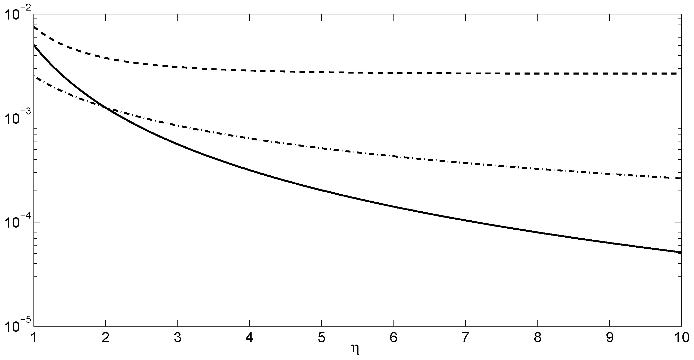
We observe that $\tilde{\Sigma }=\Sigma +\mathcal{O}\left(h\right)$, i.e., the matrix $\tilde{\Sigma }$ associated with the Euler-Maruyama method is a first order approximation of $\Sigma$. In order to appreciate the values of the errors $|{\tilde{\sigma }}_X^2-{\sigma }_X^2|$, $|{\tilde{\sigma }}_V^2-{\sigma }_V^2|$ and $|\tilde{\mu }-\mu |$ over the damping coefficient $\eta$, we depict the corresponding graphs in Figure 1. One can recognize that, for increasing values of the damping parameter, position and velocity become less correlated, as happens for the continuous problem defined by Equation (2).

Let us now analyze a genuine two-step method, i.e., the following Adams-Moulton method [16]

$${\displaystyle \mathcal{M}=\frac{1}{144+60\eta h+25g{h}^2}\tilde{\mathcal{M}},}$$

(9)

where

$$\tilde{\mathcal{M}}=\left[\begin{array}{cccc}144+60\eta h-40g{h}^2& 156h& 5g{h}^2& -12h\\ -156gh& -8(-18+12\eta h+5g{h}^2)& 12gh& h(12\eta +5gh)\\ \\ 60\epsilon h& 144\epsilon & 0& 0\end{array}\right].$$

Solving Equation (8) with respect to the $\tilde{\Sigma }$ gives

$$\tilde{\Sigma }=\left[\begin{array}{cc}\frac{90{\epsilon }^{2}h}{g(468+195\eta h-25g{h}^2)}& \frac{8640{\epsilon }^2{h}^2}{625g^2{h}^4+144{(12+5h\eta )}^2+120g{h}^2(264+25h\eta )}\\ \frac{8640{\epsilon }^2{h}^2}{625g^2{h}^4+144{(12+5h\eta )}^2+120g{h}^2(264+25h\eta )}& -\frac{2592{\epsilon }^2}{125g^2{h}^3+144\eta (-39+5h\eta )+60gh(-39+10h\eta )}\end{array}\right].$$

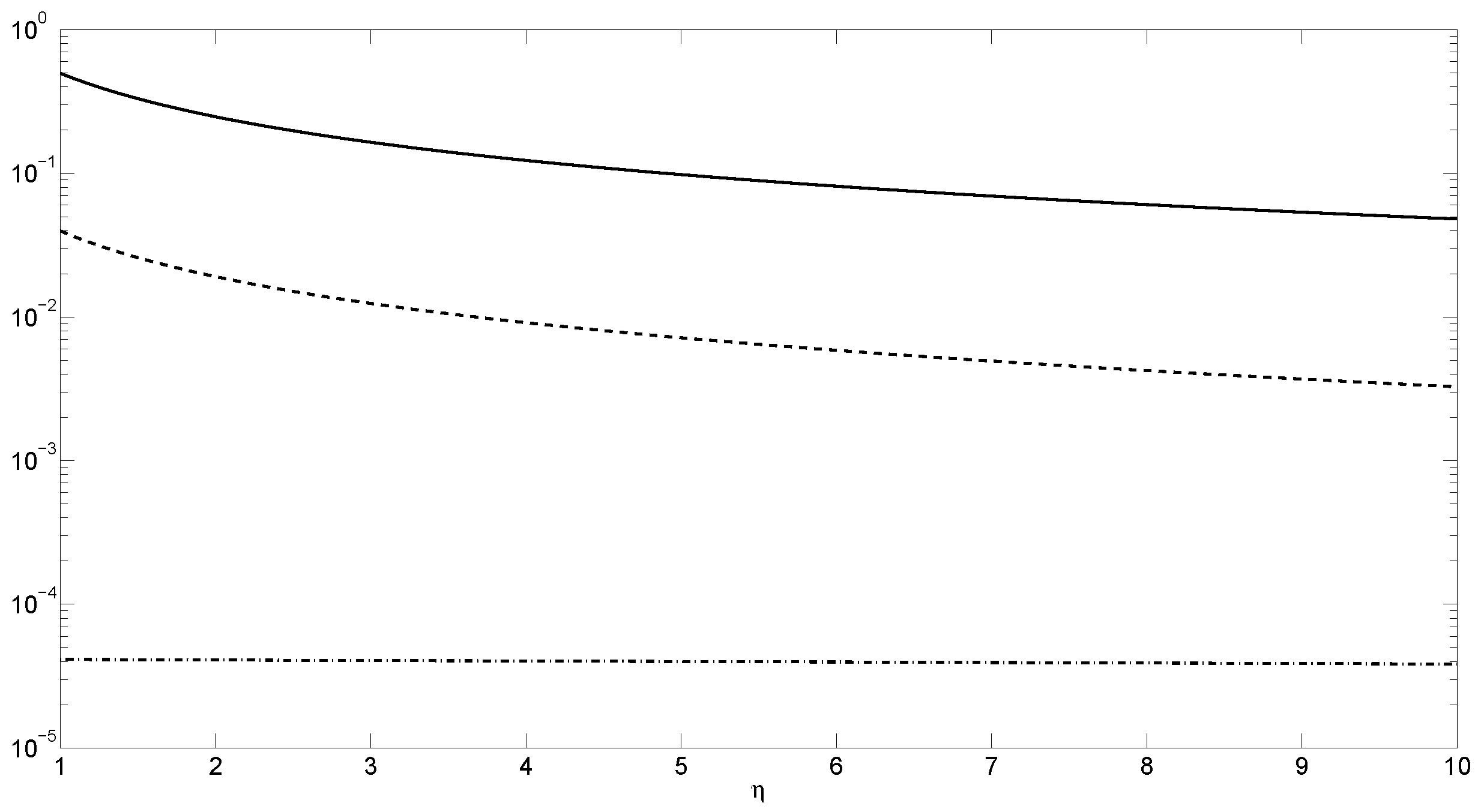
The errors $|{\tilde{\sigma }}_X^2-{\sigma }_X^2|$, $|{\tilde{\sigma }}_V^2-{\sigma }_V^2|$ and $|\tilde{\mu }-\mu |$ over the damping coefficient $\eta$, depicted in Figure 2, show that the more the problem is damped, the more the long-term mean-square of the velocity and the position are approximated with slowly decreasing errors. In the long-term, numerical position and velocity of the particle computed by the Adams-Moulton method are only weakly correlated, as desired. A qualitative comparison arising from Figure 1 and Figure 2 shows that the Euler-Maruyama method better approximates the long-term mean-square of the velocity and the position, while the Adams-Moulton method better captures the long term expectation of the product of the velocity and the position.

While the Euler-Maruyama method is able to reproduce the exact correlation matrix $\Sigma$ as h goes to 0, this is not the case for the Adams-Moulton method. This aspect opens a relevant question on the difference between one-step and genuine multistep methods. The fact that multistep methods do not recover the exact invariants of the continuous problem in the limit as h tends to 0 is typical of the deterministic setting: for instance, multistep methods do not recover the Hamiltonian function of Hamiltonian problems [17]. We conjecture that there are sources of parasitism to be properly addressed also in stochastic linear multistep methods, but this requires a very deep analysis based on the stochastic version of the backward error analysis [17], which will be an object of future investigations.

3. Stability Analysis of $\vartheta$-Methods for Stochastic Volterra Integral Equations

3.1. The Problem

We now focus our attention on stochastic Volterra integral Equations (SVIEs) in It$\widehat{\mathrm{o}}$ form

$$X_t=X_0+\underset{0}{\overset{t}{\int }}a(t,s,X_s)ds+\underset{0}{\overset{t}{\int }}b(t,s,X_s)d{W}_s,t\in [0,T].$$

(10)

The next section introduces the general class of stochastic $\vartheta$-methods [15], for which a stability analysis is provided according to the basic linear test equation,

$$X_t=X_0+\underset{0}{\overset{t}{\int }}\lambda X_{s}ds+\underset{0}{\overset{t}{\int }}\mu X_{s}d{W}_s,t\in [0,T],$$

(11)

with $\lambda ,\mu \in \mathbb{R}$, and the convolution test equation,

$$X_t=X_0+\underset{0}{\overset{t}{\int }}\left(\lambda +\sigma (t-s)\right)X_{s}ds+\underset{0}{\overset{t}{\int }}\mu X_{s}d{W}_s,t\in [0,T],$$

(12)

with $\lambda ,\mu ,\sigma \in \mathbb{R}$.

3.2. The Methodology: $\vartheta$-Methods for SVIEs

According to the classical theory on the numerical approximation of Volterra integral equations [18,19,20,21,22], we refer to the equidistant grid

$${\mathcal{I}}_h=\{t_n=nh,n=0,\dots ,N,Nh=T\}$$

and, by evaluating Equation (10) in $t_n$, we obtain

$${\displaystyle X_{t_n}=X_0+{\int }_0^{t_n}a(t_n,s,X_s)ds+{\int }_0^{t_n}b(t_n,s,X_s)d{W}_s.}$$

The stochastic $\vartheta$-method, introduced in [15], assumes the following form

$$Y_n=Y_0+h\sum _{i=0}^{n-1}\left(\vartheta a(t_n,t_{i+1},Y_{i+1})+(1-\vartheta )a(t_n,t_i,Y_i)\right)+\sqrt{h}\sum _{i=0}^{n-1}b(t_n,t_i,Y_i)G_i,$$

(13)

with $Y_0=X_0$, $h=t_{i+1}-t_i$. $G_i$ is a standard Gaussian random variable, i.e., it is $\mathcal{N}(0,1)$-distributed. Convergence analysis of the stochastic $\vartheta$-method, provided in [15] as well as in [10] for $\vartheta =0$, relies on the same hypothesis of the existence and uniqueness of the solution to Equation (10) [12,23]. In particular, the authors proved that the stochastic $\vartheta$-method is convergent with strong order $1/2$, i.e., there exists a real constant C such that

$$\mathbb{E}|X_n-Y_n{|}^2\le Ch.$$

(14)

However, as is usual in the numerical approximation of SDEs, such an order of convergence can be improved by adding further terms in the expansion of the right-hand side [11,24,25], leading to the following improved stochastic $\vartheta$-method

$$\begin{array}{cc}\hfill Y_n=Y_0& +h\sum _{i=0}^{n-1}\left(\vartheta a(t_n,t_{i+1},Y_{i+1})+(1-\vartheta )a(t_n,t_i,Y_i)\right)+\sqrt{h}\sum _{i=0}^{n-1}b(t_n,t_i,Y_i)G_{i,1}\hfill \\ & +\frac{1}{2}h\sqrt{h}\sum _{i=0}^{n-1}\frac{\partial a}{\partial x}(t_n,t_i,Y_i)b(t_i,t_i,Y_i)\left(G_{i,1}+\frac{G_{i,2}}{\sqrt{3}}\right)+\frac{1}{2}h\sum _{i=0}^{n-1}\frac{\partial b}{\partial x}(t_n,t_i,Y_i)b(t_i,t_i,Y_i)\left(G_{i,1}^2-1\right),\hfill \end{array}$$

(15)

where $\frac{\partial }{\partial x}$ denotes partial differentiation with respect to the second argument, while $G_{i,1}$ and $G_{i,2}$ are mutually independent $\mathcal{N}(0,1)$ random variables. Clearly, the numerical scheme can be made free from any derivative by suitable finite difference approximation. For instance, acting as in [11] leads to the following derivative free method

$$\begin{array}{cc}\hfill Y_n=& Y_0+h\sum _{i=0}^{n-1}\left(\vartheta a(t_n,t_{i+1},Y_{i+1})+(1-\vartheta )a(t_n,t_i,Y_i)\right)+\sqrt{h}\sum _{i=0}^{n-1}b(t_n,t_i,Y_i)G_{i,1}\hfill \\ & +\frac{h}{2}\sum _{i=0}^{n-1}\left(a(t_n,t_i,Y_i+a(t_i,t_i,Y_i)h+b(t_i,t_i,Y_i)\sqrt{h})-a(t_n,t_i,Y_i)\right)\left(G_{i,1}+\frac{G_{i,2}}{\sqrt{3}}\right)\hfill \\ & +\frac{\sqrt{h}}{2}\sum _{i=0}^{n-1}\left(b(t_n,t_i,Y_i+a(t_i,t_i,Y_i)h+b(t_i,t_i,Y_i)\sqrt{h})-b(t_n,t_i,Y_i)\right)\left(G_{i,1}^2-1\right).\hfill \end{array}$$

(16)

One can prove (see [11,15]) that the strong order of convergence of the methods defined by Equations (15) and (16) is equal to 1, since there exists a real constant K such that

$$\mathbb{E}(|X_n-Y_n{|}^2)\le K{h}^2.$$

(17)

3.3. Stability Issues

The stability analysis provided in [15] relies on investigating the behavior of the above methods when applied to the linear test Equation (11) and the convolution one (12). As regards the linear test equation, mean-square and asymptotic stability properties of the exact solution respectively occur when

$$\begin{array}{ccc}\hfill \underset{t\to \infty }{\lim }\mathbb{E}{|X\left(t\right)|}^2=0& \iff & \lambda +\frac{1}{2}{\mu }^2<0,\hfill \end{array}$$

(18)

$$\begin{array}{ccc}\hfill \underset{t\to \infty }{\lim }|X\left(t\right)|=0\mathrm{w}.\mathrm{p}.1& \iff & \lambda -\frac{1}{2}{\mu }^2<0.\hfill \end{array}$$

(19)

The following result, proved in [15], occurs.

Theorem 1.

Let $x=h\lambda$ and $y=h{\mu }^2$. The stochastic ϑ-methods defined by Equations (13), (15), (16) are mean-square stable with respect to the basic test Equation (11) if and only if

$$\left|{\alpha }^2+{\beta }^2+3{\gamma }^2+\frac{{\delta }^2}{3}+2\alpha \gamma +\beta \delta \right|<1,$$

where

(i) 

${\displaystyle \alpha =\frac{1+(1-\vartheta )x}{1-\vartheta x}}$, ${\displaystyle \beta =\frac{\sqrt{y}}{1-\vartheta x}}$, $\gamma =0$, $\delta =0$ for the method given by Equation (13);

(ii) 

${\displaystyle \alpha =\frac{1+(1-\vartheta )x-\frac{1}{2}y}{1-\vartheta x}}$, ${\displaystyle \beta =\frac{\sqrt{y}}{1-\vartheta x}}$, ${\displaystyle \gamma =\frac{y}{2(1-\vartheta x)}}$, ${\displaystyle \delta =\frac{x\sqrt{y}}{1-\vartheta x}}$ for the improved method defined by Equation (15);

(iii) 

${\displaystyle \alpha =\frac{1+(1-\vartheta )x-\frac{1}{2}\left(x\sqrt{y}+y\right)}{1-\vartheta x}}$, ${\displaystyle \beta =\frac{\sqrt{y}}{1-\vartheta x}}$, ${\displaystyle \gamma =\frac{x\sqrt{y}+y}{2(1-\vartheta x)}}$, ${\displaystyle \delta =\frac{x\sqrt{y}+x^2}{1-\vartheta x}}$ for the derivative free method given by Equation (16).

Moreover, the above methods are asymptotically stable if and only if

$$\mathbb{E}\left(\log \left|\alpha +\beta G_{n,1}+\gamma G_{n,1}^2+\delta Z_n\right|\right)<0,$$

(20)

with $Z_n=\frac{1}{2}\left(G_{n,1}+\frac{G_{n,2}}{\sqrt{3}}\right)$.

There is a strict analogy between the above presented methods and some similar formulae for SDEs. Indeed, one can see that the stability properties of the $\vartheta$-method in Equation (13) completely parallels those of the Euler-Maruyama $\vartheta$-method for SDEs [26,27,28,29,30,31]. If we remove from Equation (15) the sum involving the derivative $\frac{\partial a}{\partial x}$, we obtain

$$\begin{array}{cc}\hfill Y_n=Y_0& +h\sum _{i=0}^{n-1}\left(\vartheta a(t_n,t_{i+1},Y_{i+1})+(1-\vartheta )a(t_n,t_i,Y_i)\right)+\sqrt{h}\sum _{i=0}^{n-1}b(t_n,t_i,Y_i)G_{i,1}\hfill \\ & +\frac{1}{2}h\sum _{i=0}^{n-1}\frac{\partial b}{\partial x}(t_n,t_i,Y_i)b(t_i,t_i,Y_i)\left(G_{i,1}^2-1\right),\hfill \end{array}$$

(21)

i.e., this scheme is analogous to the Milstein $\vartheta$-method for SDEs [26], with

$${\displaystyle \alpha =\frac{1+(1-\vartheta )x-\frac{1}{2}y}{1-\vartheta x},\beta =\frac{\sqrt{y}}{1-\vartheta x},\gamma =\frac{y}{2(1-\vartheta x)},\delta =0.}$$

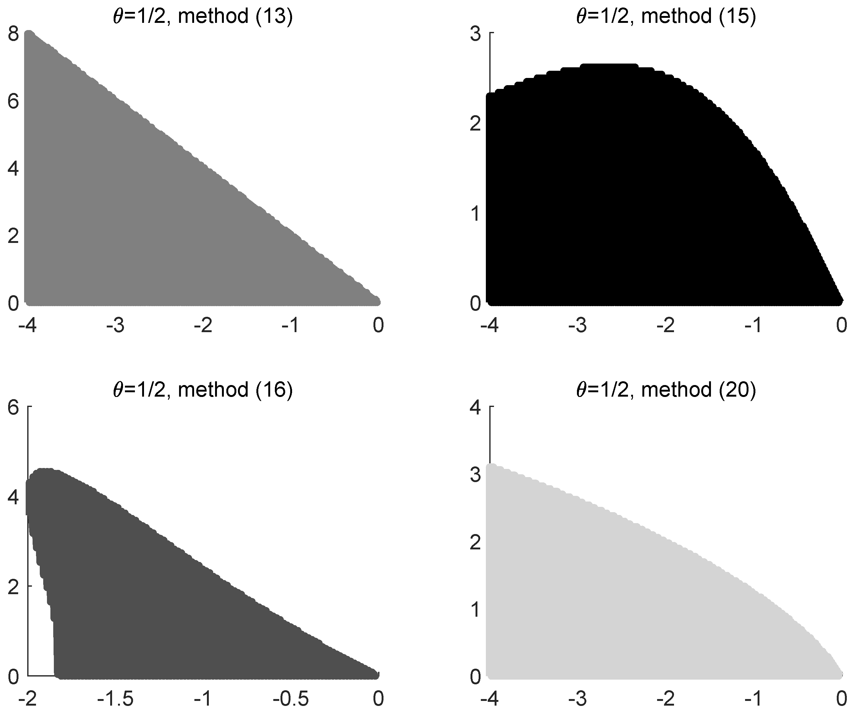
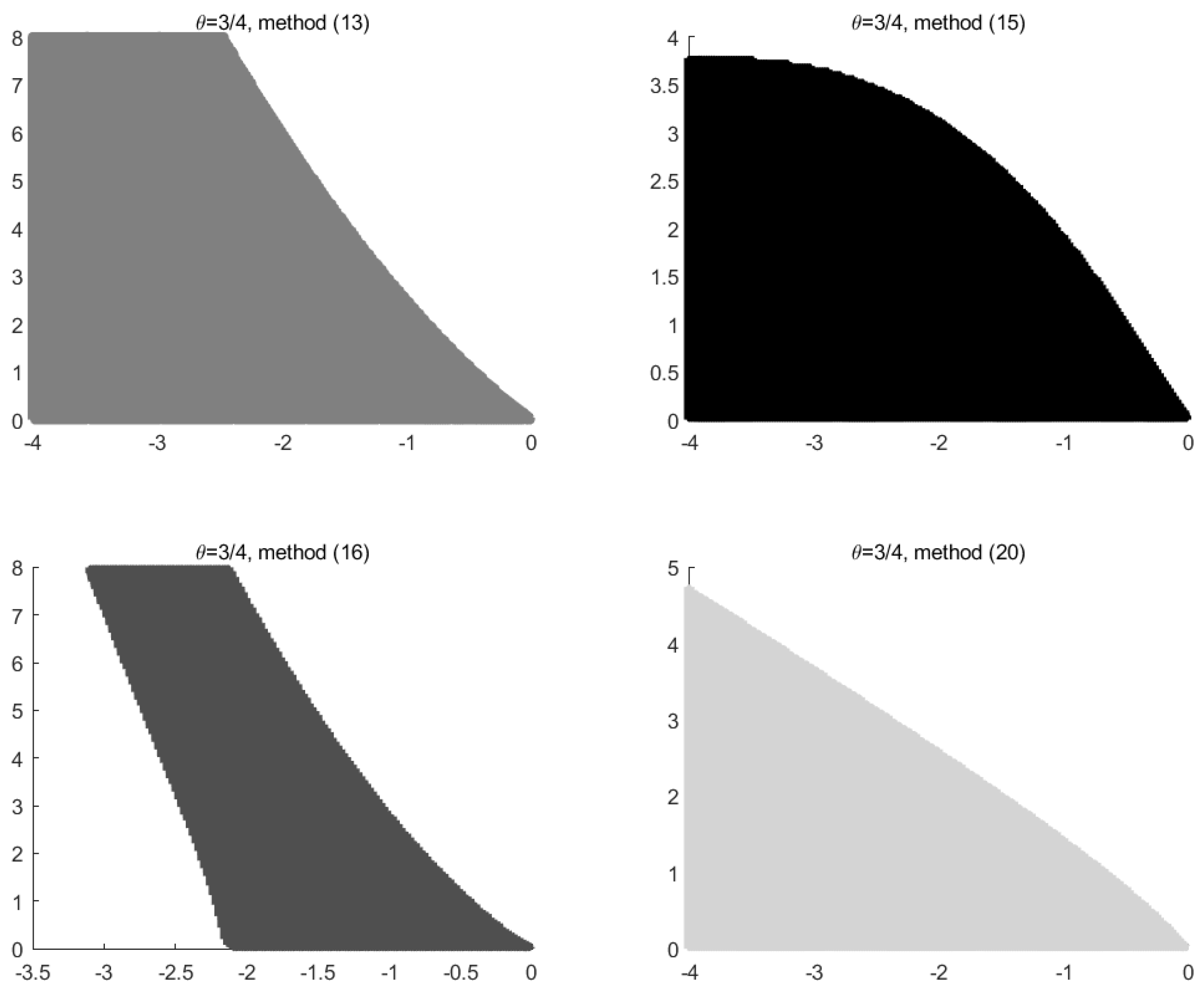
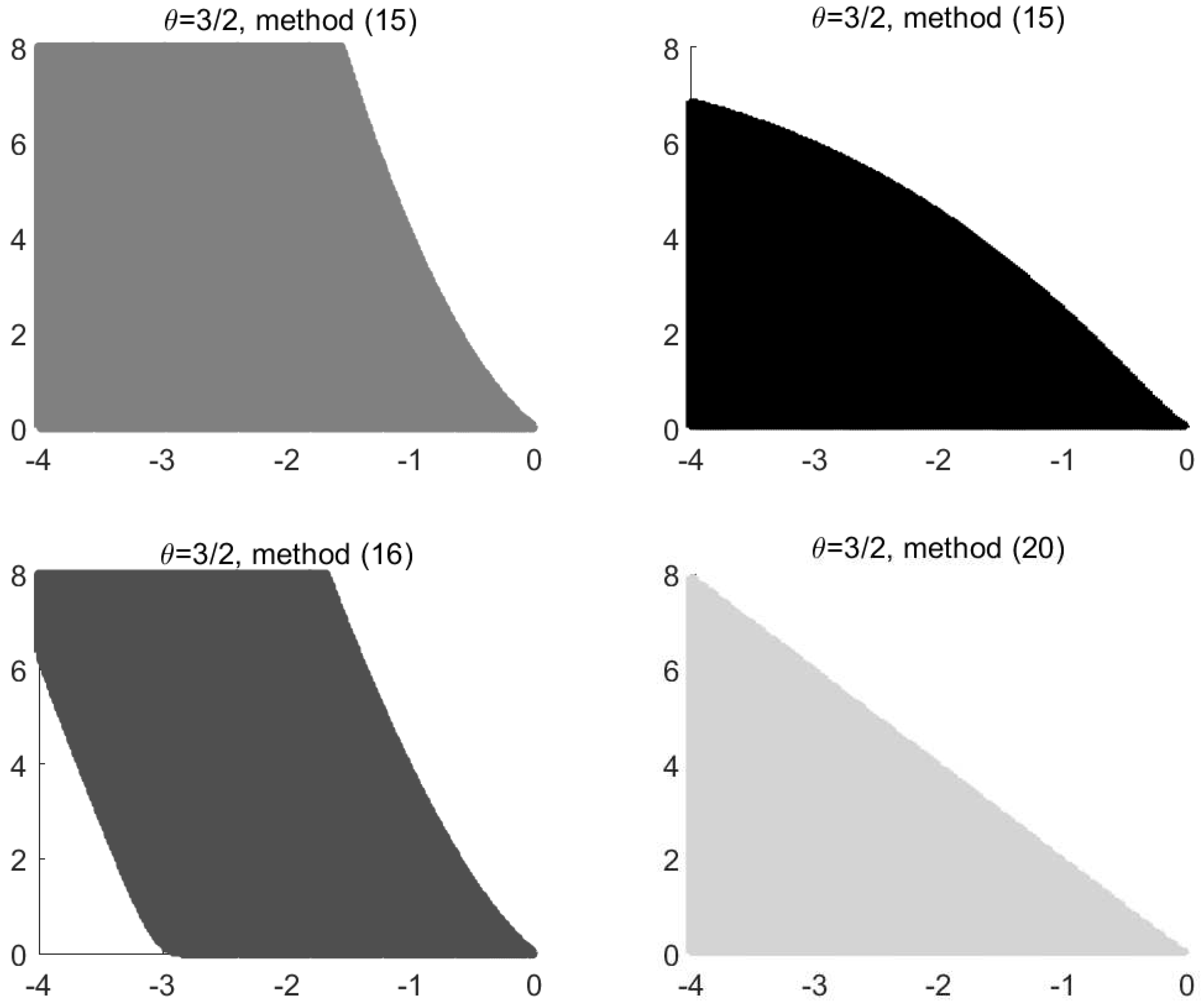
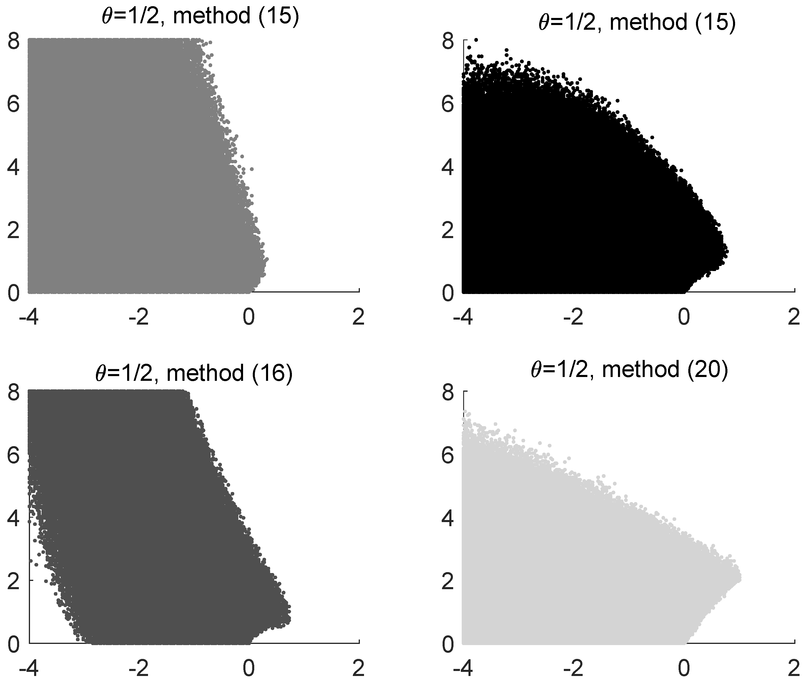
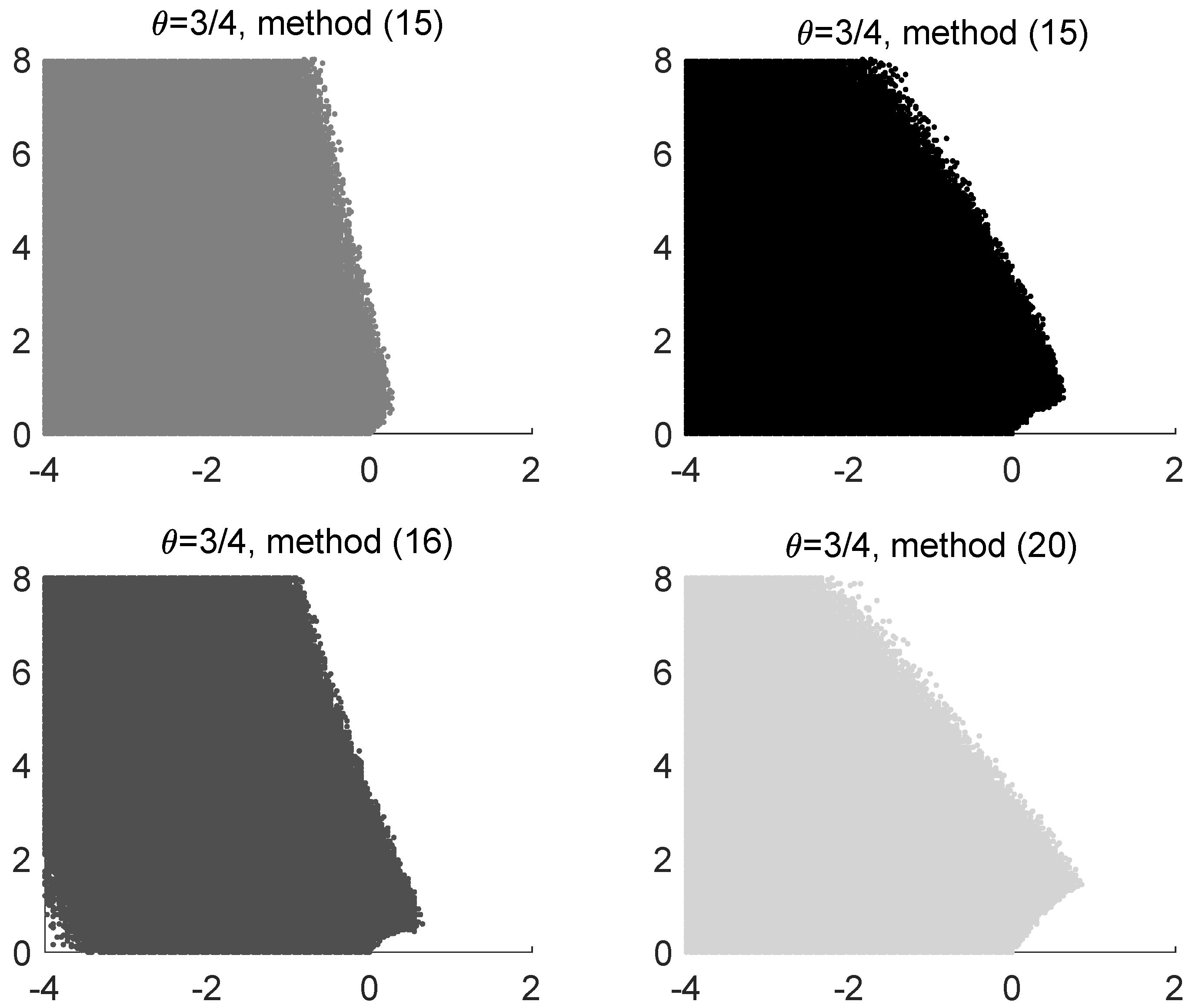
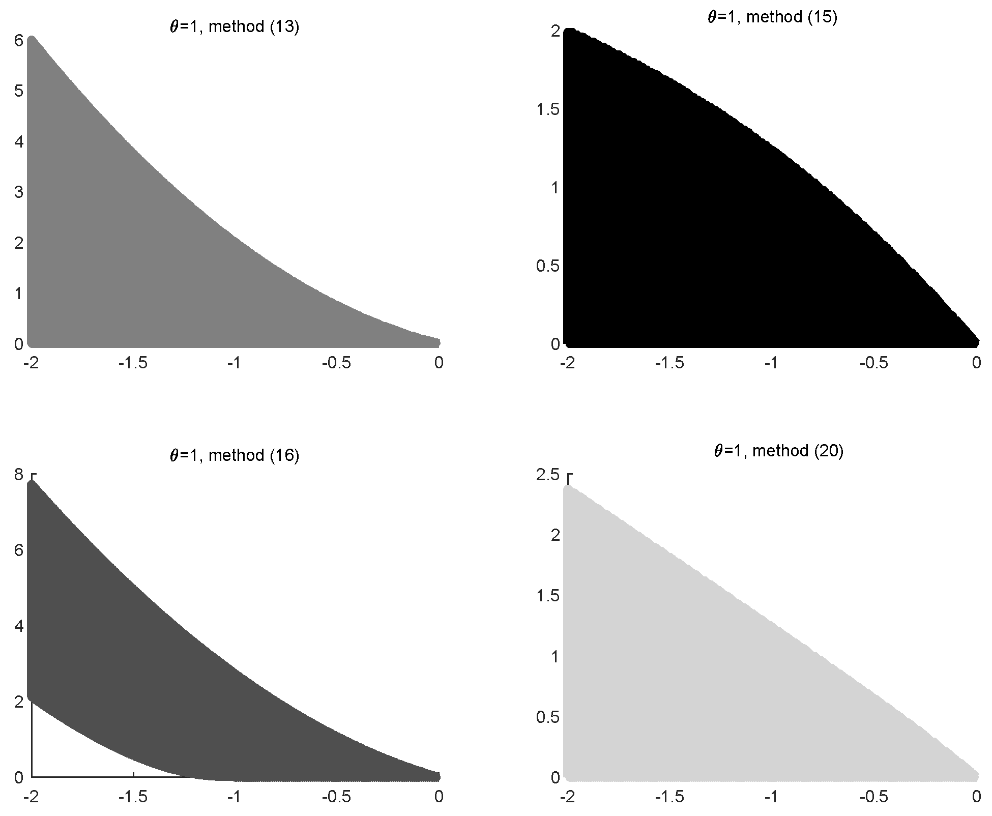
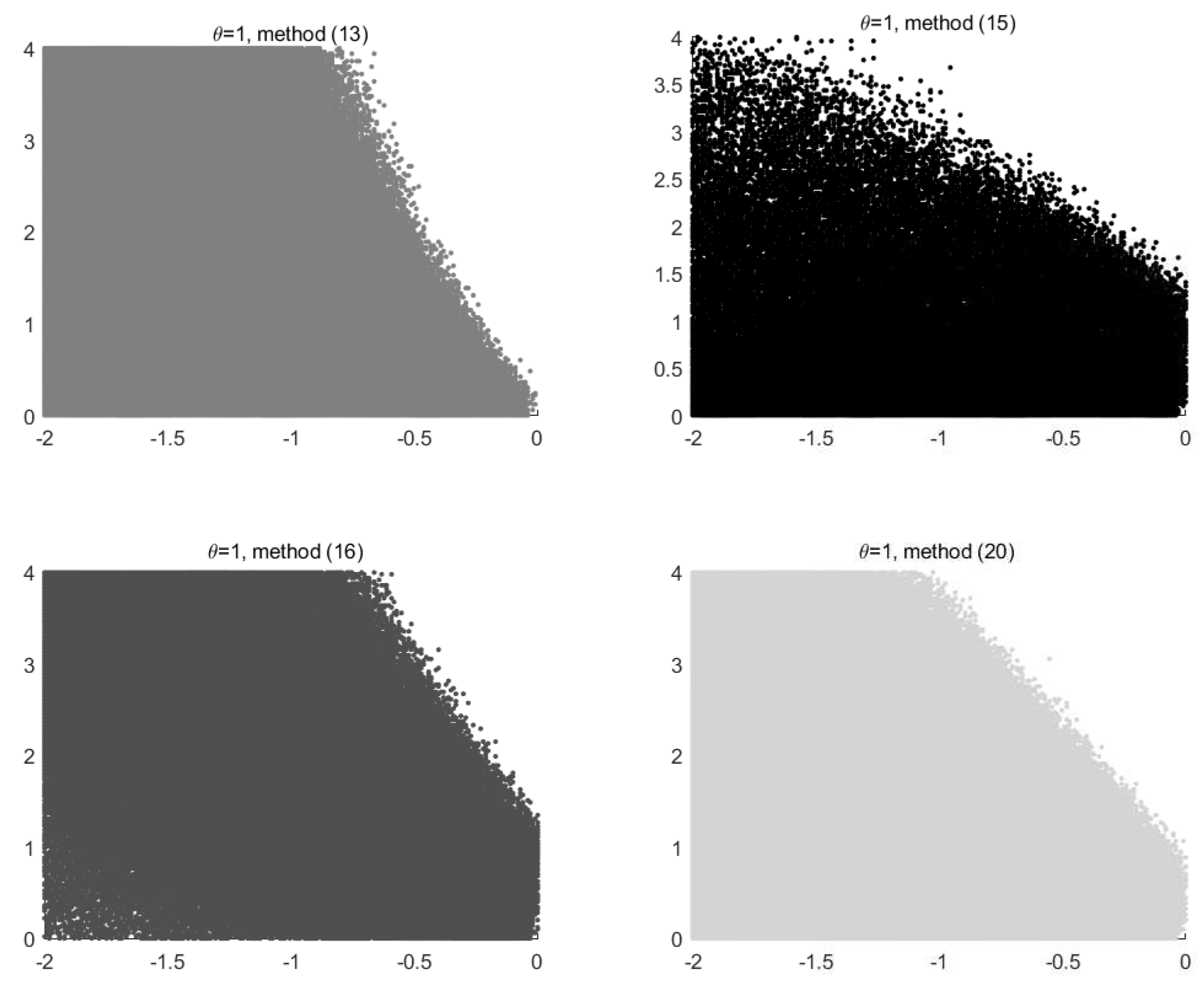
Figure 3 and Figure 4, respectively, show the regions of mean-square stability of the methods defined by Equations (13), (15), (16) and (21) with respect to the basic test Equation (11) for $\vartheta =1/2$ and $\vartheta =3/4$. Such methods, introduced in [15], can achieve unbounded stability regions in correspondence with the some values of the parameter $\vartheta \ge 1/2$. As visible from Figure 5, some methods have unbounded regions when $\vartheta >1$. Regions of asymptotic stability are depicted in Figure 6 and Figure 7, respectively, for $\vartheta =1/2$ and $\vartheta =3/4$. We observe that the regions of asymptotic stability are depicted by computing, for each point in the rectangle $[-4,2]\times [0,8]$, the value of the expectation contained in the left-hand side of the inequality (20) and checking if it is a negative number. Such expectation has been computed over 500 paths.

Let us now move to the analysis with respect to the convolution test Equation (12). The following result occurs.

Theorem 2.

Let $x=h\lambda$, $y=h{\mu }^2$ and $z=h^2\sigma$. The stochastic ϑ-methods given by Equations (13), (15), (16) and (21) are mean-square stable with respect to the convolution test Equation (12) if the spectral radius $\rho \left(K\right)$ of matrix

$$K=\left[\begin{array}{ccc}0& 0& 1\\ -\frac{\mathbb{E}\left(A_n(A_n+B_n)\right)}{{(1-\vartheta x)}^2}& -\frac{\nu }{1-\vartheta x}& \frac{\mu }{1-\vartheta x}\\ \mathbb{E}\left({\beta }_n\right)-\frac{2\mu \mathbb{E}\left(A_n(A_n+B_n)\right)}{{(1-\vartheta x)}^3}& -\frac{2\nu \mu }{{(1-\vartheta x)}^2}& \mathbb{E}\left({\alpha }_n\right)\end{array}\right]$$

(22)

is less than 1, where

$$\mu =2+(1-2\vartheta )x+z,\nu =1+(1-\vartheta )x$$

(23)

and

$${\alpha }_n={\left(\frac{\mu +A_{n+1}+B_{n+1}}{1-\vartheta x}\right)}^2,{\beta }_n={\left(\frac{\nu +A_n}{1-\vartheta x}\right)}^2,$$

where

$$A_n=\sqrt{y}{G}_{n,1}+\zeta (G_{n,1}^2-1)+\eta Z_n,B_n=\psi Z_n$$

and

(i) 

$\zeta =\eta =\psi =0$ for the method given by Equation (13),

(ii) 

$\zeta =\frac{1}{2}y$, $\eta =x\sqrt{y}$, $\psi =z\sqrt{y}$ for for the improved method given by Equation (15),

(iii) 

$\zeta =\frac{1}{2}(x\sqrt{y}+y)$, $\eta =x(x+\sqrt{y})$, $\psi =z(x+\sqrt{y})$ for the derivative free method given by Equation (16),

(iv) 

$\zeta =\frac{1}{2}y$, $\eta =0$, $\psi =z\sqrt{y}$ for the method given by Equation (21),

with $Z_n=\frac{1}{2}\left(G_{n,1}+\frac{G_{n,2}}{\sqrt{3}}\right)$.

Mean-square and asymptotic stability regions of the above methods with respect to the convolution test Equation (12) are depicted in Figure 8 and Figure 9, respectively. We observe that the region of asymptotic stability is depicted by computing, for each point in the rectangle $[-2,0]\times [0,4]$, the absolute value of the solution to Equation (12) and checking if it is smaller than a prescribed threshold, assumed equal to $1\mathrm{e}-4$ in our implementations. We also observe that larger selection of stability regions, in correspondence with different values of z and $\vartheta$, has been provided in [15].

4. Conclusions

We have presented a short review of some recent results regarding the analysis of stability issues for stochastic differential Equation (1) and stochastic Volterra integral Equation (10).

As regards SDEs, the attention has been focused on analyzing the long-term behavior of two-step methods when applied to the linear stochastic damped linear oscillator described by Equation (2). We observe that the evidence provided in Section 2 mostly focuses on the case $\eta >1$, i.e., that of strongly damped oscillators. It is very relevant to focus also on the case $\eta <<g$, characterizing weakly damped oscillators, whose relevance is high in many physical problems. This issue will be analyzed in detail in future contributions. The tool introduced in [1,2,3] gives the possibility to provide an a priori analysis relying on simple computations on 2 by 2 matrices. The structure-preserving approach to SDEs will next be devoted to stochastic Hamiltonian problems [7,8] and the stochastic extension of existing deterministic approaches [32,33,34]. A stochastic version of the non-polynomial fitting for oscillatory problems will also be addressed [35,36,37,38].

As regards SVIEs, the investigation has concerned the analysis of mean-square and asymptotic stability properties of $\vartheta$-methods, which is going to be oriented on wider families of methods, such as stochastic Runge-Kutta methods for SVIEs, in future investigations. It is also worth observing that there is a connection between stochastic integral equations and stochastic differential equations. This connection yields, for instance, to the possibility of analyzing the properties of numerical methods for SVIEs through the corresponding SDE theory. Future contributions will focus on the analysis of stability properties of numerical methods for SVIEs that inherit the stability recursion of certain methods for SDEs; this analysis is helpful to assess a stability theory of numerical methods for SVIEs, which has been partially given in Section 3.

A further relevant issue regards the employment of other test equations for the stability analysis of numerical methods for SVIEs. Indeed, it is physically relevant and interesting to consider test equations depending on exponential kernels of the type $\lambda \exp (-\sigma (t-s\left)\right)$, characteristic of system with fast response, rather than the case of the convolution test Equation (12), typical of slowly responding systems. This issues will also be addressed for stochastic fractional differential equations [35].

References

- Burrage, K.; Lenane, I.; Lythe, G. Numerical methods for second-order stochastic differential equations. SIAM J. Sci. Comput. 2007, 29, 245–264. [Google Scholar] [CrossRef] [Green Version]
- Burrage, K.; Lythe, G. Accurate stationary densities with partitioned numerical methods for stochastic differential equations. SIAM J. Numer. Anal. 2009, 47, 1601–1618. [Google Scholar] [CrossRef]
- D’Ambrosio, R.; Moccaldi, M.; Paternoster, B. Numerical preservation of long-term dynamics by stochastic two-step methods. Discret. Cont. Dyn. Syst. B 2018, 23, 2763–2773. [Google Scholar] [CrossRef]
- D’Ambrosio, R.; Moccaldi, M.; Paternoster, B.; Rossi, F. Stochastic Numerical Models of Oscillatory Phenomena. In Artificial Life and Evolutionary Computation; Pelillo, M., Poli, I., Roli, A., Serra, R., Slanzi, D., Villani, M., Eds.; Springer International Publishing: Berlin/Heidelberg, Germany, 2018; pp. 59–69. [Google Scholar]
- Schurz, H. The invariance of asymptotic laws of linear stochastic systems under discretization. Z. Angew. Math. Mech. 1999, 6, 375–382. [Google Scholar] [CrossRef]
- Strömmen Melbö, A.H.; Higham, D.J. Numerical simulation of a linear stochastic oscillator with additive noise. Appl. Numer. Math. 2004, 51, 89–99. [Google Scholar] [CrossRef] [Green Version]
- Burrage, P.M.; Burrage, K. Structure-preserving Runge-Kutta methods for stochastic Hamiltonian equations with additive noise. Numer. Algor. 2014, 65, 519–532. [Google Scholar] [CrossRef] [Green Version]
- Burrage, P.M.; Burrage, K. Low rank Runge-Kutta methods, symplecticity and stochastic Hamiltonian problems with additive noise. J. Comput. Appl. Math. 2014, 236, 3920–3930. [Google Scholar] [CrossRef] [Green Version]
- Vilmart, G. Weak second order multi-revolution composition methods for highly oscillatory stochastic differential equations with additive or multiplicative noise. SIAM J. Sci. Comput. 2014, 36, 1770–1796. [Google Scholar] [CrossRef] [Green Version]
- Wen, C.H.; Zhang, T.S. Rectangular method on stochastic Volterra equations. Int. J. Appl. Math. Stat. 2009, 14, 12–26. [Google Scholar] [CrossRef]
- Wen, C.H.; Zhang, T.S. Improved rectangular method on stochastic Volterra equations. J. Comput. Appl. Math. 2011, 235, 2492–2501. [Google Scholar] [CrossRef]
- Zhang, X. Euler schemes and large deviations for stochastic Volterra equations with singular kernels. J. Differ. Eq. 2008, 244, 2226–2250. [Google Scholar] [CrossRef]
- Higham, D.J. An algorithmic introduction to numerical simulation of stochastic differential equations. SIAM Rev. 2011, 43, 525–546. [Google Scholar] [CrossRef]
- Kloeden, P.E.; Platen, E. The Numerical Solution of Stochastic Differential Equations; Springer: Berlin/Heidelberg, Germany, 1992. [Google Scholar]
- Conte, D.; D’Ambrosio, R.; Paternoster, B. On the stability of ϑ-methods for stochastic Volterra integral equations. Discret. Cont. Dyn. Syst. B 2018, 23, 2695–2708. [Google Scholar]
- Buckwar, E.; Horvath-Bokor, R.; Winkler, R. Asymptotic mean-square stability of two-step methods for stochastic ordinary differential equations. BIT Numer. Math. 2006, 46, 261–282. [Google Scholar] [CrossRef]
- Hairer, L.; Lubich, C.; Wanner, G. Geometric Numerical Integration; Springer: Berlin/Heidelberg, Germany, 2006. [Google Scholar]
- Brunner, H.; van der Houwen, P.J. The Numerical Solution of Volterra Equations; CWI Monographs 3; North-Holland: Amsterdam, The Netherlands, 1986. [Google Scholar]
- Conte, D.; D’Ambrosio, R.; Paternoster, B. Two-step diagonally-implicit collocation based methods for Volterra integral equations. Appl. Numer. Math. 2012, 62, 1312–1324. [Google Scholar] [CrossRef]
- Conte, D.; Jackiewicz, Z.; Paternoster, B. Two-step almost collocation methods for Volterra integral equations. Appl. Math. Comput. 2008, 204, 839–853. [Google Scholar] [CrossRef]
- Conte, D.; Paternoster, B. Multistep collocation methods for Volterra integral equations. Appl. Numer. Math. 2009, 59, 1721–1736. [Google Scholar] [CrossRef]
- Cardone, A.; Conte, D. Multistep collocation methods for Volterra integro-differential equations. Appl. Math. Comput. 2013, 221, 770–785. [Google Scholar] [CrossRef]
- Wang, Z. Existence and uniqueness of solutions to stochastic Volterra equations with singular kernels and non-Lipschitz coefficients. Stat. Probab. Lett. 2008, 78, 1062–1071. [Google Scholar] [CrossRef]
- Buckwar, E.; Sickenberger, T. A comparative linear mean-square stability analysis of Maruyama- and Milstein-type methods. Math. Comput. Simul. 2011, 81, 1110–1127. [Google Scholar] [CrossRef] [Green Version]
- Saito, Y.; Mitsui, T. Stability analysis of numerical schemes for stochastic differential equations. SIAM J. Numer. Anal. 1996, 33, 2254–2267. [Google Scholar] [CrossRef]
- Bryden, A.; Higham, D.J. On the boundedness of asymptotic stability regions for the stochastic theta method. BIT 2003, 43, 1–6. [Google Scholar] [CrossRef]
- Higham, D.J. Mean-square and asymptotic stability of the stochastic theta method. SIAM J. Numer. Anal. 2000, 38, 753–769. [Google Scholar] [CrossRef]
- Ding, X.; Ma, Q.; Zhang, L. Convergence and stability of the split-step-method for stochastic differential equations. Comput. Math. Appl. 2010, 60, 1310–1321. [Google Scholar] [CrossRef]
- Higham, D.J. A-stability and stochastic mean-square stability. BIT 2000, 40, 404–409. [Google Scholar] [CrossRef]
- Hu, P.; Huang, C. The stochastic ϑ-method for nonlinear stochastic Volterra integro-differential equations. Abstr. Appl. Anal. 2014, 2014, 583930. [Google Scholar] [CrossRef]
- Shi, C.; Xiao, Y.; Zhang, C. The convergence and MS stability of exponential Euler method for semilinear stochastic differential equations. Abstr. Appl. Anal. 2012, 2012, 350407. [Google Scholar] [CrossRef]
- Butcher, J.; D’Ambrosio, R. Partitioned general linear methods for separable Hamiltonian problems. Appl. Numer. Math. 2017, 117, 69–86. [Google Scholar] [CrossRef]
- D’Ambrosio, R.; De Martino, G.; Paternoster, B. Numerical integration of Hamiltonian problems by G-symplectic methods. Adv. Comput. Math. 2014, 40, 553–575. [Google Scholar] [CrossRef]
- D’Ambrosio, R.; Izzo, G.; Jackiewicz, Z. Search for highly stable two-step Runge-Kutta methods. Appl. Numer. Math. 2012, 62, 1361–1379. [Google Scholar] [CrossRef]
- Burrage, K.; Cardone, A.; D’Ambrosio, R.; Paternoster, B. Numerical solution of time fractional diffusion systems. Appl. Numer. Math. 2017, 116, 82–94. [Google Scholar] [CrossRef]
- D’Ambrosio, R.; De Martino, G.; Paternoster, B. General Nystrom methods in Nordsieck form: Error analysis. J. Comput. Appl. Math. 2016, 292, 694–702. [Google Scholar] [CrossRef]
- D’Ambrosio, R.; Paternoster, B.; Santomauro, G. Revised exponentially fitted Runge–Kutta–Nyström methods. Appl. Math. Lett. 2014, 30, 56–60. [Google Scholar] [CrossRef]
- D’Ambrosio, R.; Moccaldi, M.; Paternoster, B. Adapted numerical methods for advection-reaction-diffusion problems generating periodic wavefronts. Comput. Math. Appl. 2017, 74, 1029–1042. [Google Scholar] [CrossRef]
Figure 1.
Graphs of (continuous line), (dashed line) and (dashed-dotted line) over , for the Euler-Maruyama method applied to Equation (2), with , , .
Figure 2.
Graphs of (continuous line), (dashed line) and (dashed-dotted line, the lowest one) over , for the Adams–Moulton method applied to Problem (2), with , , .
Figure 3.
Mean-square stability regions in the ()-plane with respect to the basic test Equation (11), case . The values of x and y are given in Theorem 1.
Figure 4.
Mean-square stability regions in the ()-plane with respect to the basic test Equation (11), case .
Figure 5.
Figure 6.
Asymptotic stability regions in the ()-plane with respect to the basic test Equation (11), case .
Figure 7.
Figure 8.
Mean-square stability regions in the ()-plane with respect to the convolution test Equation (12) for and .
Figure 9.
Asymptotic stability regions in the ()-plane with respect to the convolution test Equation (12) for and .
© 2018 by the authors. Licensee MDPI, Basel, Switzerland. This article is an open access article distributed under the terms and conditions of the Creative Commons Attribution (CC BY) license (http://creativecommons.org/licenses/by/4.0/).
Share and Cite
MDPI and ACS Style
Cardone, A.; Conte, D.; D’Ambrosio, R.; Paternoster, B. Stability Issues for Selected Stochastic Evolutionary Problems: A Review. Axioms 2018, 7, 91. https://doi.org/10.3390/axioms7040091
AMA Style
Cardone A, Conte D, D’Ambrosio R, Paternoster B. Stability Issues for Selected Stochastic Evolutionary Problems: A Review. Axioms. 2018; 7(4):91. https://doi.org/10.3390/axioms7040091
Chicago/Turabian StyleCardone, Angelamaria, Dajana Conte, Raffaele D’Ambrosio, and Beatrice Paternoster. 2018. "Stability Issues for Selected Stochastic Evolutionary Problems: A Review" Axioms 7, no. 4: 91. https://doi.org/10.3390/axioms7040091
Note that from the first issue of 2016, this journal uses article numbers instead of page numbers. See further details here.