A Quantum Adiabatic Algorithm for Multiobjective Combinatorial Optimization ^†

Abstract

In this work we show how to use a quantum adiabatic algorithm to solve multiobjective optimization problems. For the first time, we demonstrate a theorem proving that the quantum adiabatic algorithm can find Pareto-optimal solutions in finite-time, provided some restrictions to the problem are met. A numerical example illustrates an application of the theorem to a well-known problem in multiobjective optimization. This result opens the door to solve multiobjective optimization problems using current technology based on quantum annealing.

1. Introduction

Currently, quantum computation has many practical applications in engineering and computer science like machine learning, bioinformatics and artificial intelligence [1]. At the core of all these applications, there is an optimization procedure, and the quantum adiabatic computing paradigm of Farhi et al. [2] is the best method known thus far for optimization problems.

In this work, we show how to use a quantum adiabatic algorithm in multiobjective combinatorial optimization problems or MCO. An optimization problem is said to be “multiobjective” or “multicriteria” if there are two or more objective functions involved [3]. When these objective functions are required to be optimized at the same time, the optimality of solutions must be revised and, thus, an MCO can have a set of so-called “Pareto-optimal solutions” where no solution is better than any other. Here we show that the quantum adiabatic algorithm can find Pareto-optimal solutions in finite time, provided certain restrictions are met. In Theorem 2 we identify two structural features that a given MCO must satisfy in order to make an effective use of the quantum adiabatic algorithm presented in this work.

Even though most known quantum adiabatic optimization algorithms consider single-objective optimization problems (see [1,4]), only a few works discuss quantum algorithms for MCOs. Those few algorithms make use of Grover’s search method [5,6] as a subrutine that is invoked inside a classical algorithm. Alanis et al. [7] presented a quantum optimization algorithm in the context of routing problems. In [8], a general algorithm for MCO was presented and experimentally compared against a state-of-the-art metaheuristic. Both papers [7,8] use Grover’s search algorithm to solve an MCO; however, Grover’s algorithm is not naturally constructed for optimization problems. Having Grover’s algorithm as the main subrutine for optimization gives place to an “ad hoc” heuristic method whose finite time convergence has not yet been proved. Hence, these previous works [7,8] relied on numerical experiments instead of rigorous proofs.

This work presents the first quantum algorithm for MCO that guarantees finite time converge to a Pareto-optimal solution. Furthermore, since our method is constructed on the quantum adiabatic paradigm, it can be implemented in current technologies based on quantum annealing [1,9]. An extended abstract of this work appeared in [10].

The outline of this paper is as follows. In Section 2 and Section 3 we present the main concepts of MCO and adiabatic quantum computing that are relevant for this paper. In Section 4 we formally state our main result and present a full proof. In Section 5 we present a small numerical example of an MCO. Finally, in Section 6 we conclude this paper.

2. Preliminaries on Multiobjective Combinatorial Optimization

We present here the notation used throughout this paper. We also briefly review the main concepts of multiobjective optimization, which are standard definitions and can be found in several papers in the literature, for example [3]. Definitions 3, 4, 5 and 9 and Lemmas 1 and 3 are originals of this work.

The set of natural numbers (including 0) is denoted $\mathbb{N}$, the set of integers is $\mathbb{Z}$, the set of real numbers is denoted $\mathbb{R}$ and the set of positive real numbers is ${\mathbb{R}}^{+}$. For any $i,j\in \mathbb{Z}$, with $i<j$, we let ${[i,j]}_{\mathbb{Z}}$ denote the discrete interval $\{i,i+1,\dots ,j-1,j\}$. The set of binary words of length n is denoted ${\{0,1\}}^n$. We also let $\mathrm{poly}\left(n\right)=O\left(n^c\right)$ be a polynomial in n, i.e., $c\in \mathbb{N}$.

A multiobjective combinatorial optimization problem (MCO) is an optimization problem involving multiple objectives over a finite set of feasible solutions. These objectives typically present trade-offs among solutions and in general, there is no single optimal solution but a set of compromise solutions known as the Pareto set [3]. In this work, we follow the definition of Kung et al. [11]. Furthermore, with no loss of generality, all optimization problems considered in this work are minimization problems.

Let $S_1,\dots ,S_d$ be totally ordered sets and let ${\le }_i$ be an order on set $S_i$ for each $i\in {[1,d]}_{\mathbb{Z}}$. We also let $n_i$ be the cardinality of $S_i$. Define the natural partial order relation ≺ over the cartesian product $S_1\times \cdots \times S_d$ in the following way. For any $u=(u_1,\dots ,u_d)$ and $v=(v_1,\dots ,v_d)$ in $S_1\times \cdots \times S_d$, we write $u\prec v$ if and only if for any $i\in {[1,d]}_{\mathbb{Z}}$ it holds that $u_i{\le }_i{v}_i$; otherwise we write $u\nprec v$. An element $u\in S$ is a minimal element if there is no $v\in S$ such that $v\prec u$ and $v\ne u$. Moreover, we say that u is non-comparable with v if $u\nprec v$ and $v\nprec u$ and succinctly write $u\sim v$. In the context of multiobjective optimization, the relation ≺ as defined here is often referred to as the Pareto-order relation [11].

Definition 1.

An MCO is defined as a tuple $\mathsf{\Pi }=(D,R,d,\mathcal{F},\prec )$ where D is a finite set called domain, $R\subseteq {\mathbb{R}}^{+}\cup \left\{0\right\}$ is a set of real values, d is a positive integer, $\mathcal{F}$ is a finite collection of functions ${\left\{f_i\right\}}_{i\in {[1,d]}_{\mathbb{Z}}}$ where each $f_i$ maps from D to R, and ≺ is the Pareto-order relation on $R^d$ (here $R^d$ is the d-fold cartesian product on R). We also define a function f that maps D to $R^d$ as $f\left(x\right)=(f_1\left(x\right),\dots ,f_d\left(x\right))$ referred to as the objective vector of Π. If $f\left(x\right)$ is a minimal element of $R^d$, we say that x is a Pareto-optimal solution of Π. The set of all Pareto-optimal solutions of Π is denoted $P\left(\mathsf{\Pi }\right)$.

Definition 2.

For any two elements $x,y\in D$, if $f\left(x\right)\prec f\left(y\right)$ we write $x\prec y$; similarly, if $f\left(x\right)\sim f\left(y\right)$ we write $x\sim y$. For any $x,y\in D$, if $x\prec y$ and $y\prec x$ we say that x and y are equivalent and it is denoted as $x\equiv y$.

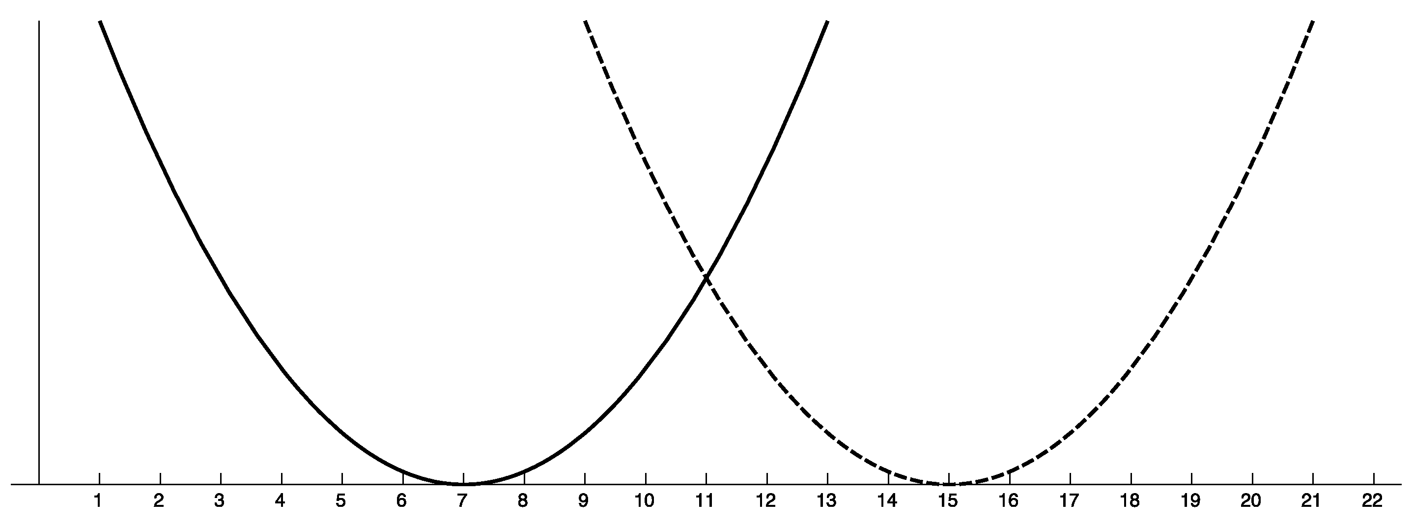
A typical example of a multiobjective optimization problem is the two-parabolas problem of Figure 1. In this problem we have two continuous objective functions defined by two parabolas that intersect in a single point.

The set of Pareto-optimal solutions can be very large, and therefore, most methods for MCOs are concerned with finding a subset of the Pareto-optimal solutions, or an approximation. Optimal query algorithms were discovered by Kung et al. [11] where all Pareto-optimal solutions can be found for $d=2,3$ and proved almost tight upper and lower bounds for any $d\ge 4$ up to polylogarithmic factors. Papadimitriou and Yannakakis [12] initiated the field of approximation algorithms for MCOs where an approximation to all Pareto-optimal solutions can be found in polynomial time.

For the remainder of this work, ≺ will always be the Pareto-order relation and will be omitted from the definition of any MCO. Furthermore, for convenience, we will often write ${\mathsf{\Pi }}_d=(D,R,\mathcal{F})$ as a short-hand for $\mathsf{\Pi }=(D,R,d,\mathcal{F})$. In addition, we will assume that each function $f_i\in \mathcal{F}$ is polynomial-time computable and each $f_i\left(x\right)$ is bounded by a polynomial in the number of bits of x. This is a typical assumption in the theory of optimization algorithms in order to have the computational complexity of any optimization algorithm to depend only on the number of “black-box” accesses to the objective function.

Definition 3.

Given any MCO ${\mathsf{\Pi }}_d$ we say that ${\mathsf{\Pi }}_d$ is well-formed if and only if for each $f_i\in \mathcal{F}$ there is a unique $x\in D$ such that $f_i\left(x\right)=0$.

Definition 4.

An MCO ${\mathsf{\Pi }}_d$ is normal if and only if ${\mathsf{\Pi }}_d$ is well-formed and $f_i\left(x\right)=0$ and $f_j\left(y\right)=0$, for $i\ne j$, implies $x\ne y$.

In a normal MCO, the value of an optimal solution in each $f_i$ is 0, and all optimal solutions are different. In Figure 1, solutions $x=7$ and $x=15$ are optimal solutions of $f_1$ and $f_2$ with value 0, respectively; hence, the two-parabolas problem of Figure 1 is normal.

Definition 5.

An MCO ${\mathsf{\Pi }}_d$ is collision-free if given $\lambda =({\lambda }_1,\dots ,{\lambda }_d)$, with each ${\lambda }_i\in {\mathbb{R}}^{+}$, for any $i\in {[1,d]}_{\mathbb{Z}}$ and any pair $x,y\in D$, with $x\ne y$, it holds that $|f_i\left(x\right)-f_i\left(y\right)|\ge {\lambda }_i$. If ${\mathsf{\Pi }}_d$ is collision-free we write succinctly as ${\mathsf{\Pi }}_d^{\lambda }$.

The two-parabolas problem of Figure 1 is not collision-free; for example, for solutions $x=5$ and $x=9$ we have that $f_1\left(5\right)=f_1\left(9\right)$.

Definition 6.

A Pareto-optimal solution x is trivial if x is an optimal solution of some $f_i\in \mathcal{F}$.

In Figure 1, solutions $x=$ 7 and $x=15$ are trivial Pareto-optimal solutions, whereas any x between seven and 15 is non-trivial.

Lemma 1.

For any normal MCO ${\mathsf{\Pi }}_d$, if x and y are trivial Pareto-optimal solutions of ${\mathsf{\Pi }}_d$, then x and y are not equivalent.

Proof. 

Let $x,y$ be two trivial Pareto-optimal solutions of ${\mathsf{\Pi }}_d$. There exists $i,j$ such that $f_i\left(x\right)=0$ and $f_j\left(y\right)=0$. Since ${\mathsf{\Pi }}_d$ is normal we have that $x\ne y$ and $f_i\left(y\right)>0$ and $f_j\left(x\right)>0$, hence, $x\sim y$ and they are not equivalent. □

Let $W_d$ be a set of of normalized vectors in ${[0,1)}^d$, the continuous interval between zero and less than one, defined as

$$W_d=\left\{w=(w_1,\dots ,w_d)\in {[0,1)}^d|\sum _{i=1}^d{w}_i=1\right\}.$$

(1)

For any $w\in W_d$, define $\langle f\left(x\right),w\rangle =\langle f\left(x\right),w\rangle =w_1{f}_1\left(x\right)+\dots +w_d{f}_d\left(x\right)$. In the literature of multiobjective optimization, if each $f_i$ is an objective function of an MCO ${\mathsf{\Pi }}_d$, it is said that $\langle f\left(x\right),w\rangle$ is a linearization or scalarization of ${\mathsf{\Pi }}_d$ [13].

The following fact is a well-known property of MCOs.

Lemma 2.

Let ${\mathsf{\Pi }}_d=(D,R,\mathcal{F})$. For any $w\in W_d$ there exists $x\in D$ such that if $\langle f\left(x\right),w\rangle ={min}_{y\in D}\left\{\langle f\left(y\right),w\rangle \right\}$, then x is a Pareto-optimal solution of ${\mathsf{\Pi }}_d$.

Proof. 

Fix $w\in W_d$ and let $x\in D$ be such that $\langle f\left(x\right),w\rangle$ is minimum among all elements of D. For any $y\in D$, with $y\ne x$, we need to consider two cases: (1) $\langle f\left(y\right),w\rangle =\langle f\left(x\right),w\rangle$ and (2) $\langle f\left(y\right),w\rangle >\langle f\left(x\right),w\rangle$.

Case (1). Here we have another two subcases, either $f_i\left(y\right)=f_i\left(x\right)$ for all i or there exists at least one pair $i,j\in \{1,\dots ,d\}$ such that $w_i{f}_i\left(x\right)<w_i{f}_i\left(y\right)$ and $w_j{f}_j\left(y\right)<w_j{f}_j\left(x\right)$. When $f_i\left(x\right)=f_i\left(y\right)$ for each $i=1,\dots ,d$ we have that x and y are equivalent. On the contrary, if $w_i{f}_i\left(x\right)<w_i{f}_i\left(y\right)$ and $w_j{f}_j\left(y\right)<w_j{f}_j\left(x\right)$, we have that $f_i\left(x\right)<f_i\left(y\right)$ and $f_j\left(y\right)<f_j\left(x\right)$, and hence, $x\sim y$.

Case (2). In this case, there exists $i\in \{1,\dots ,d\}$ such that $w_i{f}_i\left(x\right)<w_i{f}_i\left(y\right)$, and hence, $f_i\left(x\right)<f_i\left(y\right)$. Thus, $f\left(y\right)\nprec f\left(x\right)$ and $y\nprec x$ for any $y\ne x$.

We conclude from Case (1) that $x\equiv y$ or $x\sim y$, and from Case (2) that $y\nprec x$. Therefore, x is Pareto-optimal. □

Given any linearization of an MCO, by Lemma 2, an optimal solution of a linearized MCO corresponds to a Pareto-optimal solution; however, it does not hold in general that each Pareto-optimal solution has a corresponding linearization, i.e., no all Pareto-optimal solutions can always be found using linearizations.

Lemma 3.

Given ${\mathsf{\Pi }}_d=(D,R,\mathcal{F})$, any two elements $x,y\in D$ are equivalent if and only if for all $w\in W_d$ it holds that $\langle f\left(x\right),w\rangle =\langle f\left(y\right),w\rangle$.

Proof. 

Assume that $x\equiv y$. Hence $f\left(x\right)=f\left(y\right)$. If we pick any $w\in W_d$ we have that

$$\langle f\left(x\right),w\rangle =w_1{f}_1\left(x\right)+\cdots +w_d{f}_d\left(x\right)=w_1{f}_1\left(y\right)+\cdots +w_d{f}_d\left(y\right)=\langle f\left(y\right),w\rangle .$$

Now suppose that for all $w\in W_d$ it holds $\langle f\left(x\right),w\rangle =\langle f\left(y\right),w\rangle$. By contradiction, assume that $x\not\equiv y$. With no loss of generality, assume further that there is exactly one $i\in {[1,d]}_{\mathbb{Z}}$ such that $f_i\left(x\right)\ne f_i\left(y\right)$. Hence

$$w_i(f_i\left(x\right)-f_i\left(y\right))=\sum _{j\ne i}{w}_j(f_j\left(y\right)-f_j\left(x\right)).$$

(2)

The right hand of Equation (2) is 0 because for all $j\ne i$ we have that $f_j\left(x\right)=f_j\left(y\right)$. The left hand of Equation (2), however, is not 0 by our assumption, hence, a contradiction. Therefore, x is equivalent to y. □

In this work, we are only interested in finding non-trivial Pareto-optimal solutions. Finding trivial elements can be done by optimizing each $f_i$ independently; consequently, in Equation (1) we do not allow for any $w_i$ to be 1.

Definition 7.

The set of supported Pareto-optimal solutions denoted $S\left(\mathsf{\Pi }\right)$ is defined as the set of Pareto-optimal solutions x where $\langle f\left(x\right),w\rangle$ is optimal for some $w\in W_d$.

From Lemma 2, we know that some Pareto-optimal solutions cannot be found using any linearization $w\in W_d$.

Definition 8.

The set of non-supported Pareto-optimal solutions is the set $N\left(\mathsf{\Pi }\right)=P\left(\mathsf{\Pi }\right)\backslash S\left(\mathsf{\Pi }\right)$.

Note that there may be Pareto-optimal solutions x and y that are non-comparable and $\langle f\left(x\right),w\rangle =\langle f\left(y\right),w\rangle$ for some $w\in W_d$. That is equivalent to saying that the objective function obtained from a linearization of an MCO is not one-to-one (injective).

Definition 9.

Any two elements $x,y\in D$ are weakly-equivalent if and only if there exists $w\in W_d$ such that $\langle f\left(x\right),w\rangle =\langle f\left(y\right),w\rangle$.

By Lemma 3, any two equivalent solutions $x,y$ are also weakly-equivalent; on the other hand, if x and y are weakly-equivalent it does not imply that they are equivalent. For example, consider two objective vectors $f\left(x\right)=(1,2,3)$ and $f\left(y\right)=(1,3,2)$. Clearly, x and y are not equivalent; however, if $w=(1/3,1/3,1/3)$ we can see that x and y are indeed weakly-equivalent. In Figure 1, points $x=10$ and $x=12$ are weakly-equivalent.

3. The Quantum Adiabatic Algorithm

The quantum adiabatic computing paradigm was discovered by Farhi et al. [2] and the quantum adiabatic algorithm was designed to solve single-objective optimization problems. The main idea behind quantum adiabatic algorithms is that optimization problems are somehow encoded into time-dependent Hamiltonians. Then, we start the algorithm with an easy-to-prepare quantum state and we let the system evolve according to the adiabatic theorem. After some time, we measure the system and obtain an optimal solution to our optimization problem. In this work, we follow the definition of McGeoch [1].

Given an objective function f where each element in its domain can be represented with $poly\left(n\right)$ bits, a quantum adiabatic algorithm for f is constructed from three components:

• an initial Hamiltonian $H_0$ chosen in such a way that its ground state is easy to prepare;
• a final Hamiltonian $H_1$ encodes the function f in such a way that the minimum eigenvalue of $H_1$ corresponds to $f\left(x\right)$ and its ground-state corresponds to x;
• an adiabatic evolution path, that is, a function $s\left(t\right)$ that decreases from 1 to 0 as the time t goes from 0 to a given time T. In this work, we will always use a linear path $s\left(t\right)=1-t/T$.

The time-dependent Hamiltonian H for the algorithm is thus defined as

$$H\left(t\right)=s\left(t\right)H_0+(1-s\left(t\right))H_1.$$

(3)

If $|\psi (t)\rangle$ is an eigenvector of $H\left(t\right)$ that corresponds to the minimum eigenvalue, the quantum adiabatic algorithm works as follows. Prepare the system in state $|\psi (0)\rangle$ and let it evolve according to the Schrödinger’s equation. After some time T, measure the state $|\psi (T)\rangle$ with respect to some well-defined basis. The adiabatic theorem says that if T is large enough and H is non-degenerate in its minimum eigenvalue, the quantum state that is observed from the measurement is very close to $|\psi (T)\rangle$.

One of the most recent versions of the adiabatic algorithm is due to Ambainis and Regev [14] where a lower bound in the value of T can be estimated. Below we transcribe the complete statement of their theorem since it is one of the main pieces in our proof. Let $H\left(s\right)$ be a time-dependent Hamiltonian with a linear path $s=1-t/T$ for some given T. Let $\parallel H\parallel ={max}_{s\in [0,1]}\parallel H\left(s\right)\parallel$ where $\parallel ·\parallel$ is the operator norm with respect to the ${\ell }_2$-norm, and let $H^{\prime }$ and $H^{\prime \prime }$ be the first and second derivatives of H, respectively.

Theorem 1 

(Ambainis and Regev [14]). Let $H\left(s\right)$, $0\le s\le 1$, be a time-dependent Hamiltonian, let $|\psi (s)\rangle$ be one of its eigenstates, and let $\gamma \left(s\right)$ be the corresponding eigenvalue. Assume that for any $s\in [0,1]$, all other eigenvalues of $H\left(s\right)$ are either smaller that $\gamma \left(s\right)-\lambda$ or larger than $\gamma \left(s\right)+\lambda$. Consider the adiabatic evolution given by H and $|\psi (s)\rangle$ applied for time T. Then, the following condition is enough to guarantee that the final state is at distance at most δ from $|\psi (1)\rangle$:

$$T\ge \frac{{10}^5}{{\delta }^2}·max\left\{\frac{{\parallel H\parallel }^3}{{\lambda }^4},\frac{\parallel H^{\prime }\parallel ·\parallel H^{\prime \prime }\parallel }{{\lambda }^3}\right\}.$$

One of the main design decisions for adiabatic algorithms is choosing an adequate initial Hamiltonian. To make use of the adiabatic theorem, we need to construct an initial Hamiltonian that does not commute with the final Hamiltonian; otherwise, the eigenvalue gap will disappear [2].

4. Main Result of This Work

With all the technical definitions established, now we are ready to formally state our main result. For any vector w in Euclidian space we define the ${\ell }_1$-norm of w as ${\parallel w\parallel }_1=|w_1|+\cdots |w_d|$.

Theorem 2.

Let ${\mathsf{\Pi }}_d^{\lambda }$ be any normal and collision-free MCO. If there are no equivalent Pareto-optimal solutions, then for any $w\in W_d$ there exists $w^{\prime }\in W_d$ and a Hamiltonian $H_{w^{\prime }}$, satisfying $\parallel w-w^{\prime }{\parallel }_1\le 1/\mathrm{poly}\left(n\right)$, such that the quantum adiabatic algorithm, using $H_{w^{\prime }}$ as final Hamiltonian, can find a Pareto-optimal solution x corresponding to w in finite time.

In the following subsections we present a proof of Theorem 2. In Section 4.1 we show how to construct the initial and final Hamiltonians, and in Section 4.2 we show that our construction is correct.

4.1. The Initial and Final Hamiltonians for MCOs

In this section we show how to construct the initial and final Hamiltonians. Given any normal and collision-free MCO ${\mathsf{\Pi }}_d^{\lambda }=(D,R,\mathcal{F})$, assume with no loss of generality that the domain of the objective functions is $D={\{0,1\}}^n$, that is, the set of al bit strings of length n.

For each $i\in {[1,d]}_{\mathbb{Z}}$ we define a Hamiltonian $H_{f_i}={\sum }_{x\in {\{0,1\}}^n}f\left(x\right)|x\rangle \langle x|$. Since ${\mathsf{\Pi }}_d^{\lambda }$ is collision-free and normal, each $H_{f_i}$ is nondegenerate in all its eigenvalues and its minimum eigenvalue is 0. Given a linearization w of ${\mathsf{\Pi }}_d^{\lambda }$, we construct the final Hamiltonian $H_w$ for our quantum algorithm as

$$\begin{array}{cc}\hfill H_w& =w_1{H}_{f_1}+\cdots +w_d{H}_{f_d}\hfill \\ & =\sum _{x\in {\{0,1\}}^n}\langle f\left(x\right),w\rangle |x\rangle \langle x|.\hfill \end{array}$$

(4)

Now we construct the initial Hamiltonian, which cannot commute with the final Hamiltonian recently defined. In this work we make use of the Hamiltonian defined in [2]. Let $|\widehat{0}\rangle =(|0\rangle +|1\rangle )/\sqrt{2}$ and $|\widehat{1}\rangle =(|0\rangle -|1\rangle )/\sqrt{2}$. The operation F that makes $|\widehat{0}\rangle =F|0\rangle$ and $|\widehat{1}\rangle =F|1\rangle$ is called the Walsh-Hadamard transform. Thus, for any $x\in {\{0,1\}}^n$ we can make $|\widehat{x}\rangle =F^{\otimes n}|x\rangle$, where F is the n-fold Walsh–Hadamard transform. The initial Hamiltonian is

$$H_0=\sum _{x\in {\{0,1\}}^n}h\left(x\right)|\widehat{x}\rangle \langle \widehat{x}|,$$

(5)

where $h\left(0^n\right)=0$ and $h\left(x\right)=1$ for any $x\ne 0^n$.

Now that we have defined our initial and final Hamiltonians we need to show that the interpolating hamiltonian $H\left(t\right)$ of Equation (3) is indeed nondegenerate in all its eigenvalues and that it fulfils the requirements of Theorem 2.

4.2. Analysis of the Final Hamiltonian

Note that if the initial Hamiltonian does not commute with the final Hamiltonian, it suffices to prove that the final Hamiltonian is nondegenerate in its minimum eigenvalue [2]. For the remaining of this work, we let ${\sigma }_w$ and ${\alpha }_w$ be the smallest and second smallest eigenvalues of $H_w$ corresponding to a normal and collision-free MCO ${\mathsf{\Pi }}_d^{\lambda }=(D,R,\mathcal{F})$.

Lemma 4.

Let x be a non-trivial Pareto-optimal solution of ${\mathsf{\Pi }}_d^{\lambda }$. For any $w\in W_d$ it holds that ${\sigma }_w>\langle \lambda ,w\rangle$.

Proof. 

Let ${\sigma }_w=w_1{f}_1\left(x\right)+\cdots +w_d{f}_d\left(x\right)$ and let x be a non-trivial Pareto-optimal element. For each $w_i\in N$ we have that

$${\sigma }_w=\sum _i{w}_i{f}_i\left(x\right)>\sum _i{w}_i{\lambda }_i=\langle \lambda ,w\rangle .$$

 □

Lemma 5.

For any $w\in W_d$, let $H_w$ be a Hamiltonian with a nondegenerate minimum eigenvalue. The eigenvalue gap between the smallest and second smallest eigenvalues of $H_w$ is at least $\langle \lambda ,w\rangle$.

Proof. 

Let ${\sigma }_w$ be the unique minimum eigenvalue of $H_w$. We have that ${\sigma }_w=\langle f\left(x\right),w\rangle$ for some $x\in {\{0,1\}}^n$. Now let ${\alpha }_w=\langle f\left(y\right),w\rangle$ be a second smallest eigenvalue of $H_w$ for some $y\in {\{0,1\}}^n$ where $y\ne x$. Hence,

$$\begin{array}{cc}\hfill {\alpha }_w-{\sigma }_w& =\langle f\left(y\right),w\rangle -\langle f\left(x\right),w\rangle \hfill \\ & =w_1{f}_1\left(y\right)-w_1{f}_1\left(x\right)+w_2{f}_2\left(y\right)-w_2{f}_2\left(x\right)\hfill \\ & \ge w_1{\lambda }_1+w_2{\lambda }_2\hfill \\ & =\langle \lambda ,w\rangle .\hfill \end{array}$$

 □

Lemma 6.

If there are no weakly-equivalent Pareto-optimal solutions in ${\mathsf{\Pi }}_d^{\lambda }$, then the Hamiltonian $H_w$ is non-degenerate in its minimum eigenvalue.

Proof. 

By the contrapositive, suppose $H_w$ is degenerate in its minimum eigenvalue ${\sigma }_w$. Take any two degenerate minimal eigenstates $|x\rangle$ and $|y\rangle$, with $x\ne y$, such that

$$w_1{f}_1\left(x\right)+\cdots +w_d{f}_d\left(x\right)=w_1{f}_1\left(y\right)+\cdots +w_d{f}_2\left(d\right)={\sigma }_w.$$

Then it holds that x and y are weakly-equivalent. □

We further show that even if ${\mathsf{\Pi }}_d^{\lambda }$ has weakly-equivalent Pareto-optimal solutions, we can find a nondegenerate Hamiltonian. Let $m={max}_{x,i}\left\{f_i\left(x\right)\right\}$.

Lemma 7.

For any ${\mathsf{\Pi }}_d^{\lambda }$, let $x_1,\dots ,x_{\ell }\in D$ be Pareto-optimal solutions that are not pairwise equivalent. If there exists $w\in W_d$ and ${\sigma }_w\in {\mathbb{R}}^{+}$ such that $\langle f\left(x_1\right),w\rangle =\dots =\langle f\left(x_{\ell }\right),w\rangle ={\sigma }_w$ is minimum among all $y\in D$, then there exists $w^{\prime }\in W_d$ and $i\in {[1,\ell ]}_{\mathbb{Z}}$ such that for all $j\in {[1,\ell ]}_{\mathbb{Z}}$, with $j\ne i$, it holds $\langle f\left(x_i\right),w^{\prime }\rangle <\langle f\left(x_j\right),w^{\prime }\rangle$. Additionally, if the linearization $w^{\prime }$ satisfies $\parallel w-w^{\prime }{\parallel }_1\le \frac{\langle \lambda ,w\rangle }{md}$, then $\langle f\left(x_i\right),w^{\prime }\rangle$ is unique and minimum among all $\langle f\left(y\right),w^{\prime }\rangle$ for $y\in D$.

Proof. 

We prove the lemma by induction on ℓ. Let $\ell =2$, then $\langle f\left(x_1\right),w\rangle =\langle f\left(x_2\right),w\rangle$, and hence,

$$\begin{array}{cc}\hfill w_1{f}_1\left(x_1\right)+\cdots +w_d{f}_d\left(x_1\right)& ={\sigma }_w\hfill \\ \hfill w_1{f}_1\left(x_2\right)+\cdots +w_d{f}_d\left(x_2\right)& ={\sigma }_w.\hfill \end{array}$$

(6)

for some ${\sigma }_w\in {\mathbb{R}}^{+}$. From linear algebra we know that there is an infinite number of elements of $W_d$ that simultaneously satisfy Equation (6). With no loss of generality choose adequately $f_1$ and $f_2$, fix $w_3,\dots ,w_d$ and set $b_1=w_3{f}_3\left(x_1\right)+\cdots +w_d{f}_d\left(x_1\right)$ and $b_2=w_3{f}_3\left(x_2\right)+\cdots +w_d{f}_d\left(x_2\right)$. We have that

$$\begin{array}{cc}\hfill w_1{f}_1\left(x_1\right)+w_2{f}_2\left(x_1\right)& ={\sigma }_w-b_1\hfill \\ \hfill w_1{f}_1\left(x_2\right)+w_2{f}_2\left(x_2\right)& ={\sigma }_w-b_2.\hfill \end{array}$$

(7)

Again, by linear algebra, we know that Equation (7) has a unique solution $w_1$ and $w_2$; it suffices to note that the determinant of the coefficient matrix of Equation (7) is not 0, as it is proved in Appendix A.

Choose any $w_1^{\prime }\ne w_1$ and $w_2^{\prime }\ne w_2$ satisfying $w_1^{\prime }+w_2^{\prime }+w_3+\cdots +w_d=1$ and let $w^{\prime }=(w_1^{\prime },w_2^{\prime },w_3,\dots ,w_d)$. Then we have that $\langle f\left(x_1\right),w^{\prime }\rangle \ne \langle f\left(x_2\right),w^{\prime }\rangle$ because $w_1^{\prime }$ and $w_2^{\prime }$ are not solutions to Equation (7). Hence, either $\langle f\left(x_1\right),w^{\prime }\rangle$ or $\langle f\left(x_2\right),w^{\prime }\rangle$ must be smaller than the other.

Suppose that $\langle f\left(x_1\right),w^{\prime }\rangle <\langle f\left(x_2\right),w^{\prime }\rangle$. We now claim that $\langle f\left(x_1\right),w^{\prime }\rangle$ is minimum and unique among all $y\in D$. In addition to the constraint of the preceding paragraph that $w^{\prime }$ must satisfy, in order for $\langle f\left(x_1\right),w^{\prime }\rangle$ to be minimum, we must choose $w^{\prime }$ such that $\parallel w-w^{\prime }{\parallel }_1\le \frac{\langle \lambda ,w\rangle }{md}$.

Assume for the sake of contradiction the existence of $y\in D$ such that $\langle f\left(y\right),w^{\prime }\rangle \le \langle f\left(x_1\right),w^{\prime }\rangle$. Hence,

$$\langle f\left(y\right),w^{\prime }\rangle \le \langle f\left(x_1\right),w\rangle <\langle f\left(y\right),w\rangle .$$

From Lemma 4, we know that $|\langle f\left(x_1\right),w\rangle -\langle f\left(y\right),w\rangle |>\langle \lambda ,w\rangle$, and thus,

$$|\langle f\left(y\right),w^{\prime }\rangle -\langle f\left(y\right),w\rangle |>\langle \lambda ,w\rangle .$$

(8)

Using the Cauchy–Schwarz inequality we have that

$$\begin{array}{cc}\hfill |\langle f\left(y\right),w^{\prime }\rangle -\langle f\left(y\right),w\rangle |& =|\langle f\left(y\right),w^{\prime }-w\rangle |\hfill \\ & \le {\parallel f\left(y\right)\parallel }_1·{\parallel w^{\prime }-w\parallel }_1\hfill \\ & \le \langle \lambda ,w\rangle ,\hfill \end{array}$$

where the last line follows from ${\parallel f\left(y\right)\parallel }_1\le md$ and $\parallel w-w^{\prime }{\parallel }_1\le \frac{\langle \lambda ,w\rangle }{md}$; from Equation (8), however, we have that $|\langle f\left(y\right),w^{\prime }-w\rangle |>\langle \lambda ,w\rangle$, which is a contradiction. Therefore, we conclude that $\langle f\left(y\right),w^{\prime }\rangle >\langle f\left(x_1\right),w^{\prime }\rangle$ for any $y\in D$; the case for $\langle f\left(x_1\right),w^{\prime }\rangle >\langle f\left(x_2\right),w^{\prime }\rangle$ can be proved similarly. The base case of the induction is thus proved.

Now suppose the statement holds for ℓ. Let $x_1,\dots ,x_{\ell },x_{\ell +1}$ be Pareto-optimal solutions that are not pairwise equivalent. Let $w\in W_d$ be such that $\langle f\left(x_1\right),w\rangle =\cdots =\langle f\left(w_{\ell +1}\right),w\rangle$ holds. By our induction hypothesis, there exists $w^{\prime }\in W_d$ and $i\in {[1,\ell ]}_{\mathbb{Z}}$ such that $\langle f\left(x_i\right),w^{\prime }\rangle <\langle f\left(y\right),w^{\prime }\rangle$ for any other $y\in D$.

If $\langle f\left(x_i\right),w^{\prime }\rangle \ne \langle f\left(x_{\ell +1}\right),w^{\prime }\rangle$ then we are done, because either one must be smaller. Suppose, however, that $\langle f\left(x_{\ell +1}\right),w^{\prime }\rangle =\langle f\left(x_i\right),w^{\prime }\rangle ={\sigma }_{w^{\prime }}$ for some ${\sigma }_{w^{\prime }}\in {\mathbb{R}}^{+}$. From the base case of the induction we know there exists $w^{\prime \prime }\ne w^{\prime }$ that makes $\langle f\left(x_i\right),w^{\prime \prime }\rangle <\langle f\left(x_{\ell +1}\right),w^{\prime \prime }\rangle$, and hence, $\langle f\left(x_i\right),w^{\prime \prime }\rangle <\langle f\left(y\right),w^{\prime \prime }\rangle$ for any $y\in D$. Therefore, the lemma is proved. □

The premise in Lemma 7, that each $x_1,\dots ,x_{\ell }$ must be Pareto-optimal solutions, is a sufficient condition because if one solution is not Pareto-optimal, then the statement will contradict Lemma 2.

We now apply Lemma 7 to find a Hamiltonian with a nondegenerate minimum eigenvalue.

Lemma 8.

Let ${\mathsf{\Pi }}_d^{\lambda }$ be a MCO with no equivalent Pareto-optimal solutions and let $H_w$ be a degenerate Hamiltonian in its minimum eigenvalue with corresponding minimum eigenstates $|x_1\rangle ,\dots ,|x_{\ell }\rangle$. There exists $w^{\prime }\in W_d$, satisfying $\parallel w-w^{\prime }{\parallel }_1\le \frac{\langle \lambda ,w\rangle }{md}$, and $i\in {[1,\ell ]}_{\mathbb{Z}}$ such that $H_{w^{\prime }}$ is nondegenerate in its smallest eigenvalue with corresponding eigenvector $|x_i\rangle$.

Proof. 

From Lemma 6, we know that if ${\mathsf{\Pi }}_d^{\lambda }$ has no weakly-equivalent Pareto-optimal solutions, then for any w the Hamiltonian $H_w$ is nondegenerate.

We consider now the case when the minimum eigenvalue of $H_w$ is degenerate with ℓ Pareto-optimal solutions that are weakly-equivalent. Let $x_1,\dots ,x_{\ell }$ be such weakly-equivalent Pareto-optimal solutions that are non-trivial and $x_i\not\equiv x_j$ for all $i\ne j$. By Lemma 7 there exists $w^{\prime }\in W_d$, where $w\ne w^{\prime }$, such that $\langle f\left(x_i\right),w^{\prime }\rangle$ is minimum among all $y\in D$. □

If we consider our assumption from Section 2 that $m={max}_{x,i}\left\{f_i\left(x\right)\right\}$ is bounded by $\mathrm{poly}\left(n\right)$, where n is the maximum number of bits of any element in $x\in D$, by Lemma 8 we have that any $w^{\prime }$ must satisfy $\parallel w-w^{\prime }{\parallel }_1\le 1/\mathrm{poly}\left(n\right)$. Then Theorem 2 follows immediately from Lemmas 2 and 8.

To see that the adiabatic evolution takes finite-time let ${\Delta }_{max}={max}_s\parallel \frac{d}{ds}H\left(s\right)\parallel$ and $g_{min}={min}_{s}g\left(s\right)$, where $g\left(s\right)$ is the eigenvalue gap of $H\left(s\right)$. Letting $T=O\left(\frac{{\Delta }_{max}}{g_{min}^2}\right)$ suffices to find a supported solution corresponding to w. Since $g_{min}>0$ and $\parallel \frac{d}{ds}H\left(s\right)\parallel =\mathrm{poly}\left(n\right)$, we conclude that T is finite.

5. An Application to the Two-Parabolas Problem

In this section we present a numerical example on how to construct a quantum adiabatic algorithm for the two-parabolas problem. Let $T{P}_2^{\lambda }$ denote the two-parabolas problem with two objective functions and gap vector $\lambda =(0.2,0.4)$ whose description is in Appendix B. In order to use the adiabatic algorithm of Section 3 we need to consider a collision-free version of the problem.

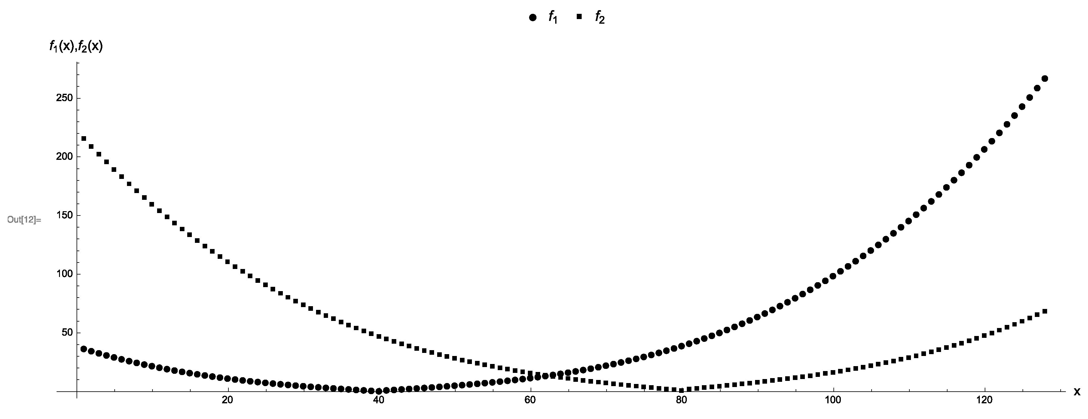
Let $n=7$ be the number of bits that are needed to encode the entire domain of each objective function. Thus, a feasible solution $x\in \{0,\dots ,127\}$. Since the gap vector is $\lambda =(0.2,0.4)$, we construct objective functions $f_1$ and $f_2$ that resemble two parabolas in such a way that for each pair of feasible solutions $x,y$ it holds that $|f_1\left(x\right)-f_1\left(y\right)|\ge 0.2$ and $|f_2\left(x\right)-f_2\left(y\right)|\ge 0.4$. See

Table A1. Complete definition of the two-parabolas example of Figure 2 for seven qubits.

x	${\mathit{f}}_1\left(\mathit{x}\right)$	${\mathit{f}}_2\left(\mathit{x}\right)$	x	${\mathit{f}}_1\left(\mathit{x}\right)$	${\mathit{f}}_2\left(\mathit{x}\right)$	x	${\mathit{f}}_1\left(\mathit{x}\right)$	${\mathit{f}}_2\left(\mathit{x}\right)$	x	${\mathit{f}}_1\left(\mathit{x}\right)$	${\mathit{f}}_2\left(\mathit{x}\right)$
0	36.14	214.879	1	34.219	208.038	2	32.375	201.354	3	30.606	194.825
4	28.91	188.449	5	27.285	182.224	6	25.729	176.148	7	24.24	170.219
8	22.816	164.435	9	21.455	158.794	10	20.155	153.294	11	18.914	147.933
12	17.73	142.709	13	16.601	137.62	14	15.525	132.664	15	14.5	127.839
16	13.524	123.143	17	12.595	118.574	18	11.711	114.13	19	10.87	109.809
20	10.07	105.609	21	9.309	101.528	22	8.585	97.564	23	7.896	93.715
24	7.24	89.979	25	6.615	86.354	26	6.019	82.838	27	5.45	79.429
28	4.906	76.125	29	4.385	72.924	30	3.885	69.824	31	3.404	66.823
32	2.94	63.919	33	2.491	61.11	34	2.055	58.394	35	1.63	55.769
36	1.214	53.233	37	0.805	50.784	38	0.401	48.42	39	0	46.139
40	0.801	43.939	41	1.205	41.818	42	1.614	39.774	43	2.03	37.805
44	2.455	35.909	45	2.891	34.084	46	3.34	32.328	47	3.804	30.639
48	4.285	29.015	49	4.785	27.454	50	5.306	25.954	51	5.85	24.513
52	6.419	23.129	53	7.015	21.8	54	7.64	20.524	55	8.296	19.299
56	8.985	18.123	57	9.709	16.994	58	10.47	15.91	59	11.27	14.869
60	12.111	13.869	61	12.995	12.908	62	13.924	11.984	63	14.9	11.095
64	15.925	10.239	65	17.001	9.414	66	18.13	8.618	67	19.314	7.849
68	20.555	7.105	69	21.855	6.384	70	23.216	5.684	71	24.64	5.003
72	26.129	4.339	73	27.685	3.69	74	29.31	3.054	75	31.006	2.429
76	32.775	1.813	77	34.619	1.204	78	36.54	0.6	79	38.54	0
80	40.621	1.2	81	42.785	1.804	82	45.034	2.413	83	47.37	3.029
84	49.795	3.654	85	52.311	4.29	86	54.92	4.939	87	57.624	5.603
88	60.425	6.284	89	63.325	6.984	90	66.326	7.705	91	69.43	8.449
92	72.639	9.218	93	75.955	10.014	94	79.38	10.839	95	82.916	11.695
96	86.565	12.584	97	90.329	13.508	98	94.21	14.469	99	98.21	15.469
100	102.331	16.51	101	106.575	17.594	102	110.944	18.723	103	115.44	19.899
104	120.065	21.124	105	124.821	22.4	106	129.71	23.729	107	134.734	25.113
108	139.895	26.554	109	145.195	28.054	110	150.636	29.615	111	156.22	31.239
112	161.949	32.928	113	167.825	34.684	114	173.85	36.509	115	180.026	38.405
116	186.355	40.374	117	192.839	42.418	118	199.48	44.539	119	206.28	46.739
120	213.241	49.02	121	220.365	51.384	122	227.654	53.833	123	235.11	56.369
124	242.735	58.994	125	250.531	61.71	126	258.5	64.519	127	266.644	67.423

for a complete definition of $T{P}_2^{\lambda }$ and Figure 2 shows a plot of all points.

We define the final and initial Hamiltonians following Equations (4) and (5), respectively. In particular, the initial Hamiltonian is defined as

$$H_0=\sum _{x\in {\{0,1\}}^n\backslash \left\{0^n\right\}}8|\widehat{x}\rangle \langle \widehat{x}|.$$

(9)

The number 8 in Equation (9) is there only to enhance the visual presentation of the plots in this paper. The Hamiltonian of the entire system for $T{P}_2^{\lambda }$ is

$$H\left(s\right)=(1-s)H_0+s{H}_w.$$

(10)

From the previous section we know that $T=O\left(\frac{{\Delta }_{max}}{g_{min}^2}\right)$ suffices to find a supported solution corresponding to w [15]. The quantity ${\Delta }_{max}$ is usually easy to estimate [2]. The eigenvalue gap $g_{min}$ is, however, very difficult to compute; indeed, determining for any Hamiltonian if $g_{min}>0$ is undecidable [16].

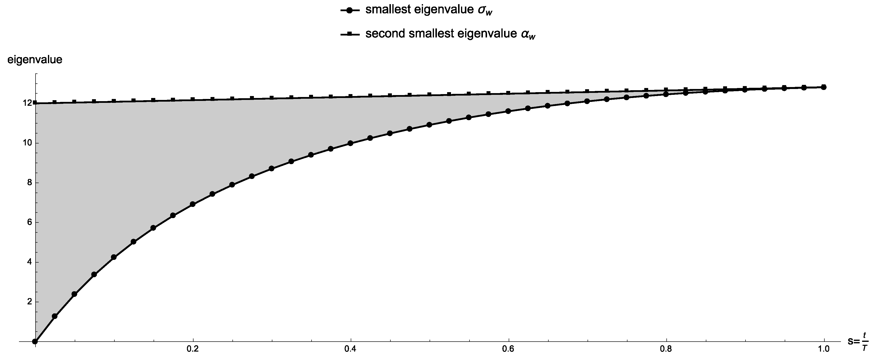
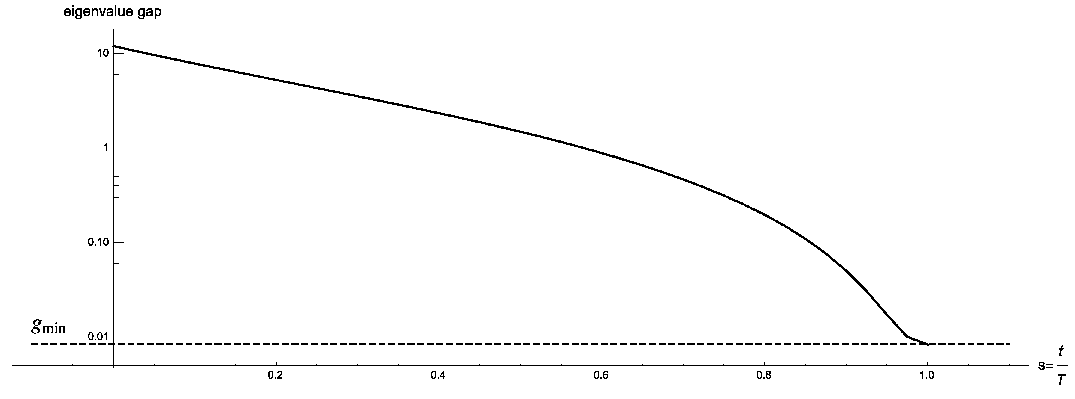
In Figure 3 we present the eigenvalue gap of $T{P}_2^{\lambda }$ for $w=0.57$ where we let $w_1=w$ and $w_2=1-w_1$; for this particular value of w the final Hamiltonian $H_w$ has a unique minimum eigenstate which corresponds to Pareto-optimal solution $x_0=59$. The two smallest eigenvalues never touch, and exactly at $s=1$ the gap is $|\langle f\left(x_0\right),w\rangle -\langle f\left(x_1\right),w\rangle |$, where $x_0=59$ and $x_1=60$ are the smallest and second smallest solutions with respect to w, which agrees with Lemmas 4 and 5. Figure 4 shows the eigenvalue gap as a function of s in a logarithmic scale.

Similar results can be observed for different values of w and a different number of qubits. Therefore, the experimental evidence lead us to conjecture that in the two-parabolas problem $g_{min}\ge |\langle f\left(x\right),w\rangle -\langle f\left(y\right),w\rangle |$, where x and y are the smallest and second smallest solutions with respect to w.

6. Concluding Remarks and Open Problems

In the last few years the field of quantum computation is finding new applications in artificial intelligence, machine learning and data analysis. These new discoveries were fueled by a deeper understanding in the foundations of quantum information and computation which resulted in new quantum algorithms for optimization problems (see for example [17]).

In this paper we addressed another side of optimization problems, namely, multiobjective optimization problems, where multiple objective functions must be optimized at the same time. This paper presented the first quantum multiobjective optimization algorithm with provable finite-time convergence. Other authors proposed quantum algorithms for multiobjective optimization [7,8] but these algorithms were ad-hoc heuristics with no theoretical guarantees for convergence. Furthermore, these aforementioned proposals utilized a hybrid approach of classical and quantum computation where Grover’s search algorithm constitutes the only “quantum part” and the other parts of the algorithm are classical. The quantum algorithm of this work is based on the successful quantum adiabatic paradigm of Farhi et al. [2] and it is a full quantum algorithm, that is, all of its execution is performed by quantum operations with no classical parts except the initialization and read-out of the results.

The quantum multiobjective optimization algorithm of this work finds a single Pareto-optimal solution and in order to find other Pareto-optimal solutions it must be executed several times. Furthermore, the main result of this work, Theorem 2, requires that all multiobjective optimization problems be normal, collision-free and with no equivalent solutions. Even though this result constrains the class of mulitiobjective problems that can be solved, this work presents a first step forward to a general purpose quantum multiobjective optimization algorithm.

We end this paper by listing a few promising and challenging open problems.

• We know from Lemma 2 that if we linearize a multiobjective optimization problem, some Pareto-optimal solutions (the non-supported solutions) may not be found. Considering that our quantum algorithm uses a linearization technique, a new mapping or embedding method of a multiobjective problem into a Hamiltonian is necessary in order to construct a quantum adiabatic algorithm that can also find supported Pareto-optimal solutions.
• For a practical application of our quantum algorithm, the linearization w in Theorem 2 must be chosen so that the resulting total Hamiltonian is non-degenerate in its ground-state. Therefore, more research is necessary in order to develop a heuristic for choosing w before executing the algorithm.
• As mentioned before, currently our algorithm is only good for multiobjective problems with no equivalent solutions. Natural multiobjective optimization problems appear in engineering and science with several equivalent solutions, and hence, in order to use our algorithm in a real-world situation we need to take into account equivalent solutions. This is a crucial point mainly because equivalent solutions yields degenerate ground-states in the total Hamiltonian, and hence, the quantum adiabatic theorem cannot be used.
• The time complexity of our quantum multiobjective algorithm depends on the spectral gap of the total Hamiltonian. Even though we presented some numerical results that suggest a polynomial execution time for the two-parabolas problem, a more thorough and rigorous approach must be done. This depends on the analysis of the spectral gap of Hamiltonians that can be constructed for specific multiobjective problems, for example, solving our conjecture for the two-parabolas problem of Section 5.

References

- Catherine, C.; McGeoch, C.C. Adiabatic Quantum Computation and Quantum Annealing: Theory and Practice; Morgan and Claypool: San Rafael, CA, USA, 2014. [Google Scholar]
- Farhi, E.; Goldstone, J.; Gutman, S.; Sipser, M. Quantum computation by adiabatic evolution. arXiv, 2000; arXiv:quant-ph/0001106. [Google Scholar]
- von Lücken, C.; Barán, B.; Brizuela, C. A survey on multi-objective evolutionary algorithms for many-objective problems. Comput. Optim. Appl. 2014, 58, 707–756. [Google Scholar] [CrossRef]
- Venegas-Andraca, S.; Cruz-Santos, W.; McGeoch, C.; Lanzagorta, M. A cross-disciplinary introduction to quantum annealing-based algorithms. Contemp. Phys. 2018, 59, 174–197. [Google Scholar] [CrossRef] [Green Version]
- Grover, L. A fast quantum mechanical algorithm for database search. In Proceedings of the 28th Annual ACM Symposium on the Theory of Computing (STOC), Philadelphia, PA, USA, 22–24 May 1996; pp. 212–219. [Google Scholar]
- Baritompa, W.P.; Bulger, D.W.; Wood, G.R. Grover’s quantum algorithm applied to global optimization. SIAM J. Optim. 2005, 15, 11701184. [Google Scholar] [CrossRef]
- Alanis, D.; Botsinis, P.; Xin Ng, S.; Lajos Hanzo, L. Quantum-Assisted Routing Optimization for Self-Organizing Networks. IEEE Access 2014, 2, 614–632. [Google Scholar] [CrossRef]
- Fogel, G.; Barán, B.; Villagra, M. Comparison of two types of Quantum Oracles based on Grover’s Adaptative Search Algorithm for Multiobjective Optimization Problems. In Proceedings of the 10th International Workshop on Computational Optimization (WCO), Federated Conference in Computer Science and Information Systems (FedCSIS), ACSIS, Prague, Czech Republic, 3–6 September 2017; Volume 11, pp. 421–428. [Google Scholar]
- Das, A.; Chakrabarti, B.K. Quantum annealing and quantum computation. Rev. Mod. Phys. 2008, 80, 1061. [Google Scholar] [CrossRef]
- Barán, B.; Villagra, M. Multiobjective optimization in a quantum adiabatic computer. Electr. Notes Theor. Comput. Sci. 2016, 329, 27–38. [Google Scholar] [CrossRef]
- Kung, H.T.; Luccio, F.; Preparata, F.P. On finding the maxima of a set of vectors. J. ACM 1975, 22, 469–476. [Google Scholar] [CrossRef]
- Papadimitriou, C.; Yannakakis, M. On the approximability of trade-offs and optimal access of web sources. In Proceedings of the 41st Annual Symposium on Foundations of Computer Science (FOCS), Washington, DC, USA, 12–14 November 2000; pp. 86–92. [Google Scholar]
- Ehrgott, M.; Gandibleux, X. A survey and annotated bibliography of multiobjective combinatorial optimization. OR Spektrum 2000, 22, 425–460. [Google Scholar] [CrossRef]
- Ambainis, A.; Regev, O. An elementary proof of the quantum adiabatic theorem. arXiv, 2004; arXiv:quant-ph/0411152. [Google Scholar]
- Wim van Dam, W.; Mosca, M.; Vazirani, U. How powerful is adiabatic quantum computation? In Proceedings of the 42nd IEEE Symposium on Foundations of Computer Science (FOCS), Las Vegas, NV, USA, 14–17 October 2001; pp. 279–287. [Google Scholar]
- Cubitt, T.; Perez-Garcia, D.; Wolf, M. Undecidability of the Spectral Gap. Nature 2015, 528, 207–211. [Google Scholar] [CrossRef] [PubMed]
- Biamonte, J.; Witteck, P.; Pancotti, N.; Rebentrost, P.; Wiebe, N.; Lloyd, S. Quantum machine learning. Nature 2017, 549, 195–202. [Google Scholar] [CrossRef] [PubMed] [Green Version]
Figure 1.
The two-parabolas Problem. The first objective function is represented by the bold line and the second objective function by the dashed line. Note that there are no equivalent elements in the domain. In this particular example, all the solutions between seven and 15 are Pareto-optimal.
Figure 2.
A discrete two-parabolas problem on seven qubits. Each objective function and is represented by the rounded points and the squared points, respectively. The gap vector is . The trivial Pareto-optimal points are 40 and 80.
Figure 3.
Eigenvalues of Equation (10) for the two-parabolas problem of Figure 2 for . The eigenvalue gap at is exactly , where and are the smallest and second smallest solutions with respect to this value of w.
Figure 4.
Logarithmic plot of the eigenvalue gap as a function of s.
© 2019 by the authors. Licensee MDPI, Basel, Switzerland. This article is an open access article distributed under the terms and conditions of the Creative Commons Attribution (CC BY) license (http://creativecommons.org/licenses/by/4.0/).
Share and Cite
MDPI and ACS Style
Barán, B.; Villagra, M. A Quantum Adiabatic Algorithm for Multiobjective Combinatorial Optimization. Axioms 2019, 8, 32. https://doi.org/10.3390/axioms8010032
AMA Style
Barán B, Villagra M. A Quantum Adiabatic Algorithm for Multiobjective Combinatorial Optimization. Axioms. 2019; 8(1):32. https://doi.org/10.3390/axioms8010032
Chicago/Turabian StyleBarán, Benjamín, and Marcos Villagra. 2019. "A Quantum Adiabatic Algorithm for Multiobjective Combinatorial Optimization" Axioms 8, no. 1: 32. https://doi.org/10.3390/axioms8010032
Note that from the first issue of 2016, this journal uses article numbers instead of page numbers. See further details here.