A New Set Theory for Analysis

Abstract

We provide a canonical construction of the natural numbers in the universe of sets. Then, the power set of the natural numbers is given the structure of the real number system. For this, we prove the co-finite topology, $Cof\left(\mathbb{N}\right)$, is isomorphic to the natural numbers. Then, we prove the power set of integers, $2^{\mathbb{Z}}$, contains a subset isomorphic to the non-negative real numbers, with all its defining structures of operations and order. We use these results to give the power set, $2^{\mathbb{N}}$, the structure of the real number system. We give simple rules for calculating addition, multiplication, subtraction, division, powers and rational powers of real numbers, and logarithms. Supremum and infimum functions are explicitly constructed, also. Section 6 contains the main results. We propose a new axiomatic basis for analysis, which represents real numbers as sets of natural numbers. We answer Benacerraf’s identification problem by giving a canonical representation of natural numbers, and then real numbers, in the universe of sets. In the last section, we provide a series of graphic representations and physical models of the real number system. We conclude that the system of real numbers is completely defined by the order structure of natural numbers and the operations in the universe of sets.

1. Introduction

In building the continuum, we make use of properties of integers and sets. Apart from this, we assume the basic concepts of category theory. Mainly, the concept of isomorphism between categories. Background knowledge on previous axiomatic constructions of the real numbers will be of help. The more modern constructions of the real number system can be found in the references [1,2,3,4,5]. It is notable that the real number system has been studied in detail through the generations, and still new insights and more useful constructions are sought. The mathematical objects that have previously been denominated as real numbers are objects of complex and illusive structure. The mathematician has always had to recur to advanced tools and objects in building the real number structure. In the words of Dr. K. Knopp [6] (p. 4)

“…these preliminary investigations are tedious and troublesome, and have actually, it must be confessed, not yet reached any entirely satisfactory conclusion at all.”

That is why real numbers are usually presented axiomatically as a set satisfying certain rules, without specifying the nature of the set nor proving its existence. In undergraduate school, constructions of the real number system are rarely taught, even in advanced courses of analysis. This leads to a certain gap in the learning of the student. This is one of our major motivations.

We are able to represent real numbers in terms of regular sets built upon the empty set, and in Section 6 we give a canonical construction for natural numbers, and real numbers as an extension of these. We also prove that the real number system is isomorphic in structure (not only cardinality) to $2^{\mathbb{N}}$. The structure of $2^{\mathbb{N}}$ can be defined artificially in terms of any bijection with $\mathbb{R}$, but that does not give us any new information or computational advantages since such bijections usually lack interpretation.

Our work is to define a structure for $2^{\mathbb{N}}$ and prove this structure is equivalent to the real number system as a totally ordered field with the property of the supremum element (completeness). We provide order and operations $<,\oplus ,\odot$ on the objects of $2^{\mathbb{N}}$, so that $\mathbb{F}a<\mathbb{F}b$ if and only if $a<b$, and $\mathbb{F}(a+b)=\mathbb{F}a\oplus \mathbb{F}b$ and $\mathbb{F}(a·b)=\mathbb{F}a\odot \mathbb{F}b$, for a bijection $\mathbb{F}:\mathbb{R}\to 2^{\mathbb{N}}$.

We first prove the closed sets of the cofinite topology of $\mathbb{N}$ are equivalent to the natural number system. We symbolize this family of sets with $Cof\left(\mathbb{N}\right)=\{A\in 2^{\mathbb{N}}|Aisfinite\}$. Then, we apply the same method to define order and operation on $2^{-\mathbb{N}}$; the continuum $[0,1]$ is isomorphic in structure to the power set of $-\mathbb{N}$. These constructions are generalized to obtain ${\mathbb{R}}^{+}$, the set of non-negative real numbers. Let ${\mathbb{Z}}^{-}=\{A\in 2^{\mathbb{Z}}|\max \left(A\right)exist\}$. Order and operations for ${\mathbb{Z}}^{-}$ are well defined. The elements of ${\mathbb{Z}}^{-}$ are called set numbers and the totality of set numbers is the totality of non-negative real numbers. In particular, the elements of $Cof\left(\mathbb{N}\right)$ and $2^{-\mathbb{N}}$ are set numbers: $Cof\left(\mathbb{N}\right),2^{-\mathbb{N}}\subset {\mathbb{Z}}^{-}$. The structures $Cof\left(\mathbb{N}\right),2^{-\mathbb{N}}$ are naturally embedded into ${\mathbb{Z}}^{-}$.

2. Motivation

Every natural number has unique representation as a sum of natural powers of 2. This expression is usually treated as a sequence of 0’s and 1’s. A 0 in the n-th place indicates that $2^n$ is not a summand in the expression. A digit 1 in that same place would indicate that $2^n$ is indeed a summand. This is the usual binary expression of natural numbers. Given the binary representation of a natural number x, we can naturally assign it a set number X. The elements of the set number are the places in the sequence with a digit 1. For example, the sequence $5=(\dots ,0,0,0,1,0,1)$ is assigned the set number $\{0,2\}$ because the 0-th and 2-nd space are occupied by the digit 1. The sequence $13=(\dots ,0,0,0,1,1,0,1)$ will be mapped to the set number $\{0,2,3\}$ and $17=(\dots ,0,0,0,1,0,0,0,1)$ is the set number $\{0,4\}$. Given set numbers $A,B$, we say $A<B$ if $\max (A▵B)\in B$, where $A▵B=(A\cup B)-(A\cap B)$ is the symmetric difference of the two sets. This order on $Cof\left(\mathbb{N}\right)$ is isomorphic to the order ${\mathbb{N}}_{\le }$.

Next, we define the sum of two set numbers in $Cof\left(\mathbb{N}\right)$; it takes the form of a recursive formula that ends in finite steps. If $X\in {\mathbb{Z}}^{-}$ is any set number, define the successor of X as $s\left(X\right)={\{i+1\}}_{i\in X}$; the new set $s\left(X\right)$ is the set of successors. The sum of $A,B\in Cof\left(\mathbb{N}\right)$ is the sum of two new set numbers $A^{\prime }\oplus B^{\prime }$, where $A^{\prime }=A▵B$ and $B^{\prime }=s(A\cap B)$. Intuitively, we add the powers of 2 that are not repeated, with the powers of 2 that are repeated. We increase by 1 the powers that are repeated because, in terms of natural numbers, it is equivalent to multiplication by 2. Thus, $A\oplus B=(A▵B)\oplus s(A\cap B)$, where the function $s:2^{\mathbb{N}}\to 2^{\mathbb{N}}$ adds 1 to the elements of the argument, specifically $s\varnothing =\varnothing$ and $s\left\{0\right\}=\left\{1\right\}$.

To illustrate with an example, $13+5=(2^0+2^2+2^3)+(2^0+2^2)=\left(2^3\right)+2\ast (2^0+2^2)=\left(2^3\right)+(2^1+2^3)=\left(2^1\right)+2\ast \left(2^3\right)=\left(2^1\right)+\left(2^4\right)=18$. In terms of set numbers, $\{0,2,3\}\oplus \{0,2\}=\left\{3\right\}\oplus \{0+1,2+1\}=\left\{3\right\}\oplus \{1,3\}=\left\{1\right\}\oplus \{3+1\}=\left\{1\right\}\oplus \left\{4\right\}=\{1,4\}\oplus \varnothing =\{1,4\}$. In general, the process ends in finite steps. The sum of two sets, $A,B$, is equal to the sum of the sets $A^{\prime }=A▵B$ and $B^{\prime }=s(A\cap B)$. The sum of these two is in turn equal to the sum of $A^{″}=A^{\prime }▵B^{\prime }$ and $B^{″}=s(A^{\prime }\cap B^{\prime })$, etc.... This process ends when $B^{\left(n\right)}$ becomes the empty set (after a finite number of iterations). We have $15+23=\{0,1,2,3\}\oplus \{0,1,2,4\}=\{3,4\}\oplus s\{0,1,2\}=\{3,4\}\oplus \{1,2,3\}=\{1,2,4\}\oplus \left\{4\right\}=\{1,2\}\oplus \left\{5\right\}=\{1,2,5\}\oplus \varnothing =\{1,2,5\}=38$.

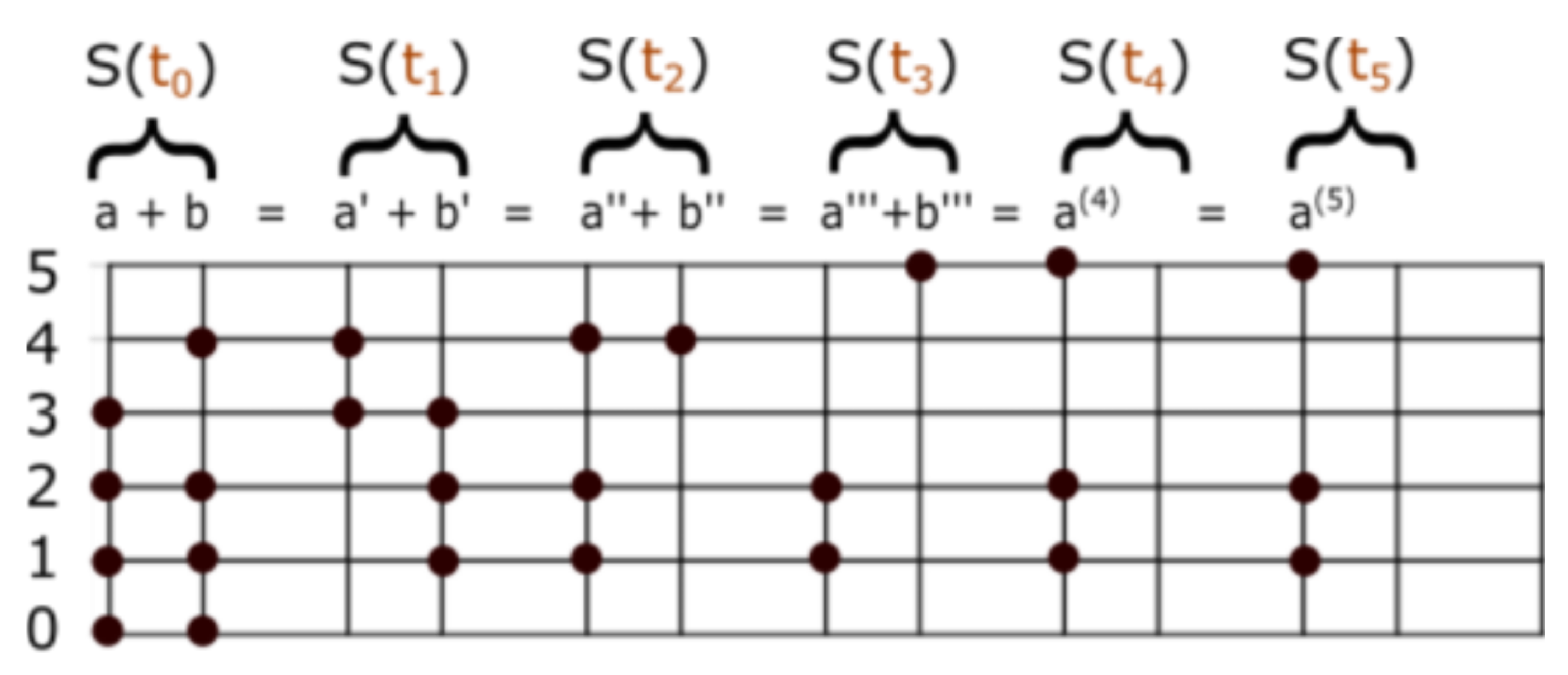
This process can be modeled with particles occupying energy levels. A set number will be represented by a column with numbered energy levels, and any given arrangement of particles occupying levels (with at most one particle on each level). To perform addition of two columns, we give one rule: two particles in the same level are replaced by a single particle, one level up. Let us describe this in detail. Given two columns $A,B$, we call the ordered pair $\mathbf{S}=(A,B)$ a state. Thus, a state is determined by two columns with occupied levels. Call the levels of the left column $A_i$ and the levels of the right column $B_j$, so that $A_4$ means the fourth level of the left column and $B_0$ means the lowest (or 0-th) level of the right column.

We provide a system that evolves discretely in time. To pass from a state $t_n$ to $t_{n+1}$, we form two new columns. The left column of state $t_{n+1}$ is occupied in the energy levels that were not repeated in the previous state $t_n$. The right column of state $t_{n+1}$ is occupied in the energy level $B_{j+1}$ if the energy levels $A_j$ and $B_j$ were both occupied during the state $t_n$. To find the set number sum of two set numbers, we merge the two columns into a single column, by applying our sum formula. The right column becomes the empty set in finite steps, and this guarantees our answer. We define $X\oplus \varnothing =\varnothing \oplus X=X$. See Figure 1.

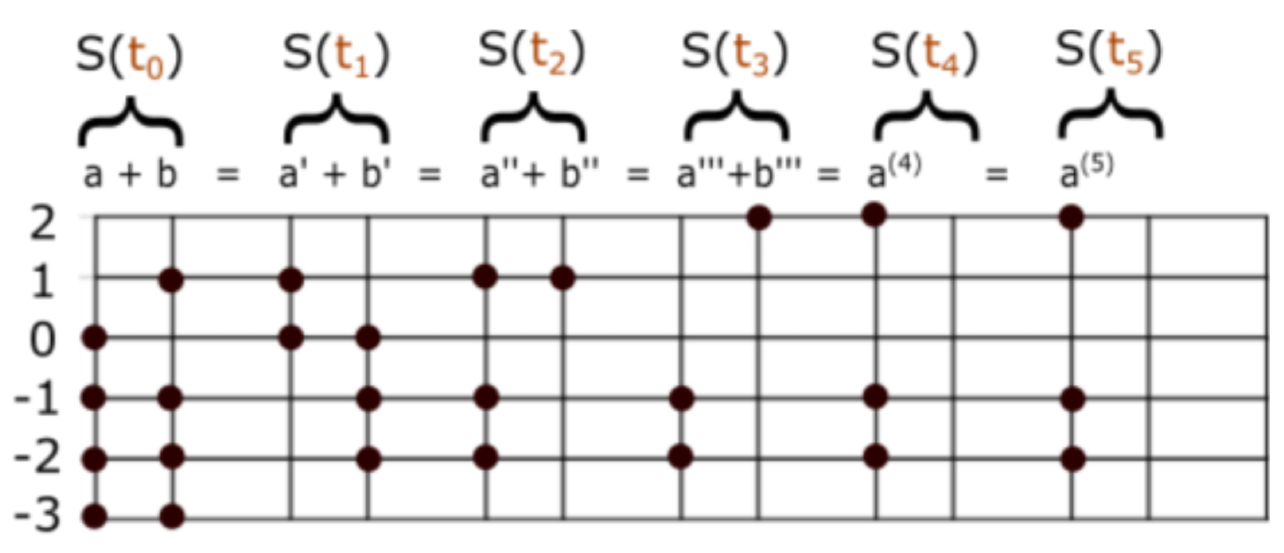
The state stabilizes in a finite number of steps (we provide an upper bound on this number). That is to say, there exists a state $\mathbf{S}\left(t_n\right)$ such that $\mathbf{S}\left(t_k\right)=\mathbf{S}\left(t_n\right)$ for all $k\ge n$. Say $A_i^n$ represents the level $A_i$ at time $t_n$. Then, stability means for all $i,j\ge 0$ and for all $n\ge k$, it is true $A_i^n=A_i^k$ and $B_j^n=0$. Notice, the same diagram is valid under vertical displacements. In Figure 2, we illustrate the fact that the same system of states of Figure 1 holds under displacement of the energy levels (Figure 2).

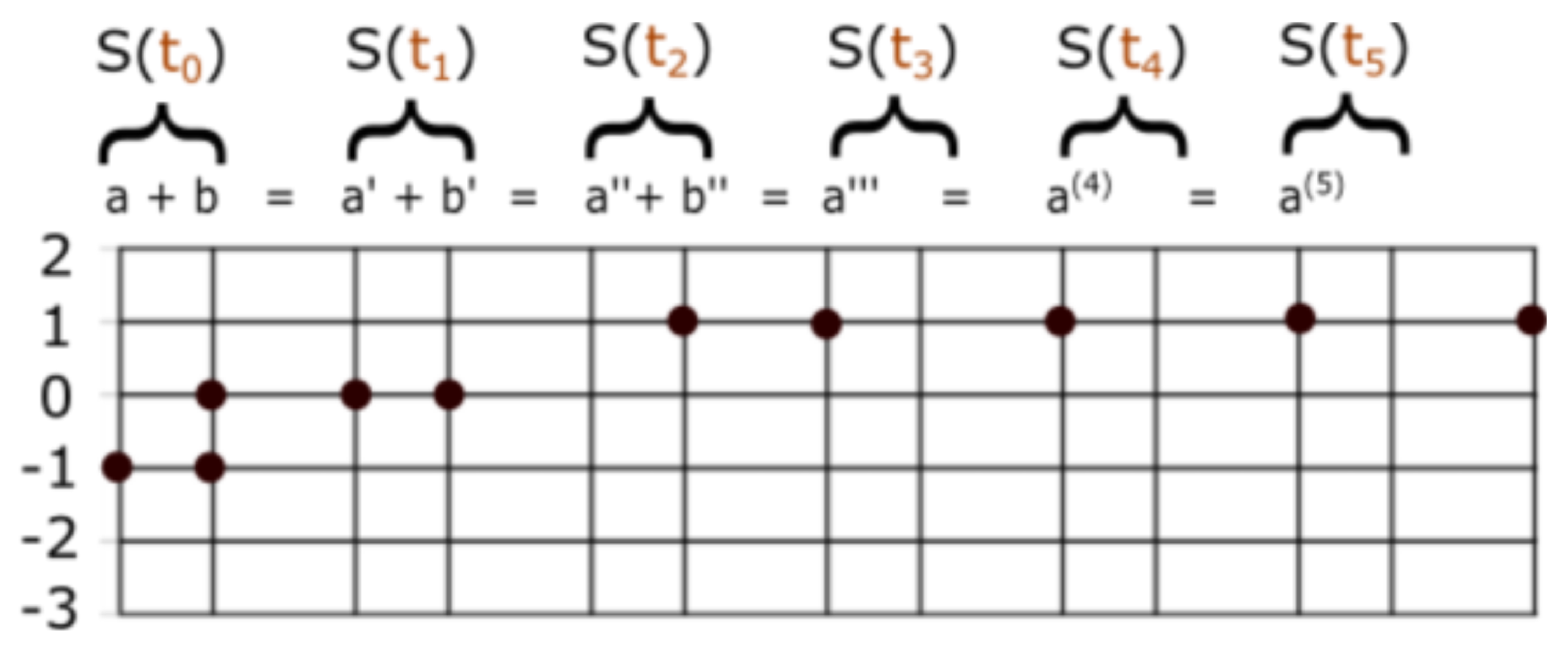
Real numbers in the unit interval are the sum of negative powers of 2. We adapt the same rules of order and operation to arbitrary sets of negative integers. For example, $\frac{1}{2}=2^{-1}=\{-1\}$, and $\frac{3}{2}=\{-1,0\}$ because $\frac{3}{2}=2^{-1}+2^0$. Adding these, $\frac{1}{2}+\frac{3}{2}=\{-1\}\oplus \{-1,0\}=\left\{0\right\}\oplus s\{-1\}=\left\{0\right\}\oplus \left\{0\right\}=\varnothing \oplus s\left\{0\right\}=s\left\{0\right\}=\left\{1\right\}=2^1$ (Figure 3).

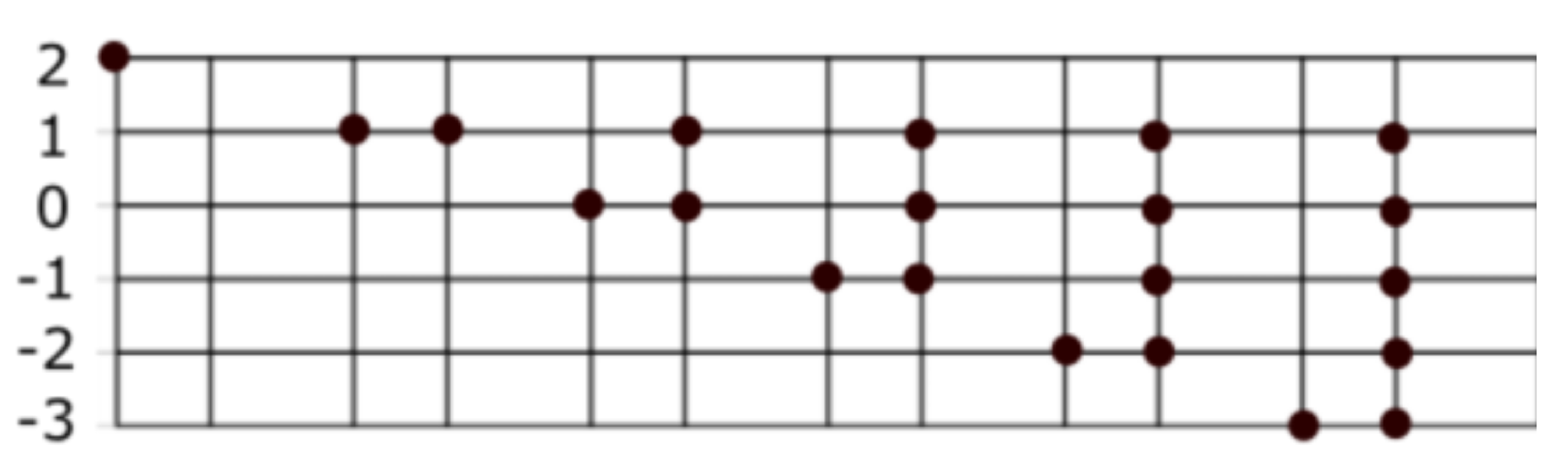
Rearranging the energy levels of Figure 3, so that $a=\left\{0\right\}$ and $b=\{0,1\}$, we get a graphic representation of $1+3=4$. Actually, in every diagram, we are representing denumerable sums (under change of levels). Observe ${\sum }_{i<k}{2}^i=2^k$, for every integer k. This is equivalent to defining ${\left\{i\right\}}_{i=-\infty }^{k-1}=\left\{k\right\}$. It comes from an iteration of Figure 3, and we will see why this is consistent (Figure 4).

3. $\mathbb{N}\cong \mathit{Cof}\left(\mathbb{N}\right)$

3.1. Order

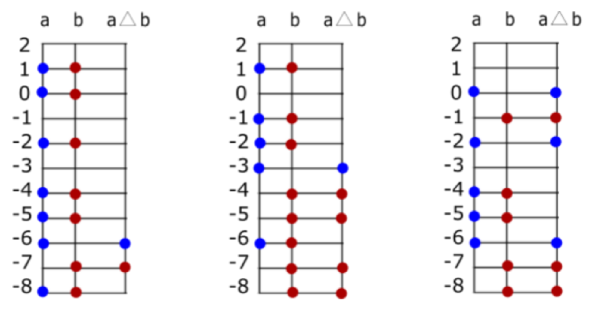
We define an order relation < between set numbers; $A<B$ if $\max (A▵B)\in B$. In the contrary case, $\max (A▵B)\in A$ and we define $B<A$. Every two set numbers are comparable because the symmetric difference is non-empty and it has a maximum. It is not difficult to see that we have a total order on the family of set numbers ${\mathbb{Z}}^{-}$. In particular, it is a well order on $Cof\left(\mathbb{N}\right)$, if we take $Cof\left(\mathbb{N}\right)$ as substructure of ${\mathbb{Z}}^{-}$. We give three examples in Figure 5.

3.2. Addition

We define the sum of two set numbers as a recursive formula that ends in finite steps; to prove our formula ends in finite steps, it is of crucial importance to suppose the cardinality of $A,B$ is finite. This formula is based on the following observation for adding powers, $2^{k+1}=2^k+2^k$. We ask ⊕ obey $\left\{i\right\}\oplus \left\{i\right\}=\{i+1\}$, for every singleton $\left\{i\right\}\in Cof\left(\mathbb{N}\right)$. The operation of addition is defined by $A\oplus B=(A▵B)\oplus s(A\cap B)$. Successive applications yield

$$\begin{array}{ccc}A\oplus B\hfill & =\hfill & (A▵B)\oplus s(A\cap B)=\left[\right(A▵B)▵s(A\cap B\left)\right]\oplus s\left[\right(A▵B)\cap s(A\cap B\left)\right]\hfill \\ \hfill & =\hfill & \left[\right((A▵B)▵s(A\cap B))▵s((A▵B)\cap s(A\cap B)\left)\right]\oplus s\left[\right((A▵B)▵s(A\cap B))\cap s((A▵B)\cap s(A\cap B)\left)\right].\hfill \end{array}$$

Before complicating things more, we stop here to see what is happening. Let $C_{n+1}=C_n▵D_n$ and $D_{n+1}=s(C_n\cap D_n)$, where $C_1=A▵B$ and $D_1=s(A\cap B)$. The previous equalities can be rewritten as

$$\begin{array}{c}\hfill A\oplus B=C_1\oplus D_1=C_2\oplus D_2=C_k\oplus D_k\end{array}$$

for all $k\in \mathbb{N}$. We are calculating $C_k\oplus D_k$ as a sum $C_{k+1}\oplus D_{k+1}$, where the term $D_{k+1}$ is dependent on the intersection. We call $D_{k+1}$ the remainder, and although it is not getting smaller in value (as natural number), the cardinality (as set number) goes to 0. However, it can be the case that the cardinality of the remainder does not get smaller. It may stay constant for finite iterations. It is guaranteed that, in a finite number of steps, the remainder becomes the empty set, and our result is now obvious. We have iterated the formula to obtain $A\oplus B=C_{k+1}\oplus D_{k+1}$, where $D_{k+1}=\varnothing$. The system stabilizes when $D_{k+1}=\varnothing$, so that $A\oplus B=C_{k+1}=C_{k+2}=\cdots =C_k\cup D_k$. The cardinalities of the remainders satisfy $\#\left(D_1\right)\ge \#\left(D_2\right)\ge \cdots \ge \#\left(D_k\right)>\#\left(D_{k+1}\right)=\#\left(D_{k+2}\right)=\cdots =0$, for some natural number k.

It is left to the reader to prove (1) $\#\left(D_k\right)=0$ in at most $\max (A\cup B)+1$ steps. (2) $A\oplus B=A\oplus \left\{b_1\right\}\oplus \left\{b_2\right\}\oplus \cdots \oplus \left\{b_k\right\},$ for any set numbers $A,B$ where the $b_i$ are the elements of B. The proofs of the algebraic properties are not all trivial. It is not trivial to prove the associative property for ⊕. The best thing to do to avoid direct proofs is to prove $\mathbb{F}(a+b)=\mathbb{F}a\oplus \mathbb{F}b$ and ${\mathbb{F}}^{-1}(A\oplus B)={\mathbb{F}}^{-1}A+{\mathbb{F}}^{-1}B$, where $\mathbb{F}$ is the bijection $\mathbb{N}\to Cof\left(\mathbb{N}\right)$ that acts by $x={\sum }_{i\in X}{2}^i\mapsto X$.

3.3. Product

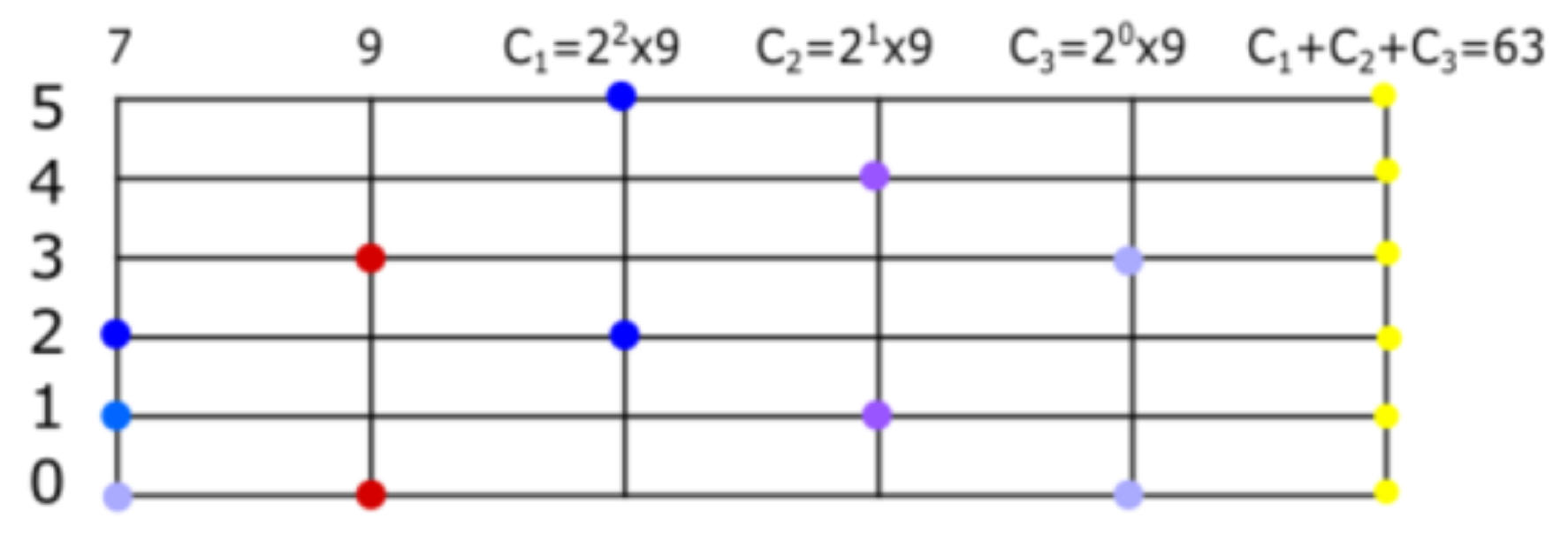
Multiplication by 2 is equivalent to adding 1 to the elements of the corresponding set number. For example, $2\ast 14=\left\{1\right\}\odot \{1,2,3\}=\{1+1,2+1,3+1\}=\{2,3,4\}=28$. In general, $2·x=s\left(X\right)$, where X is the set number corresponding to $x\in \mathbb{N}$. Recall $s\left(X\right)={\{i+1\}}_{i\in X}$. Multiplication by 4, is equivalent to adding $+2$ to all the elements of X. In general, multiplication by $2^k$ is equivalent to adding k, to the elements of X. That is to say, $2^k·x$ corresponds to the set number $\left\{k\right\}\odot X={\{i+k\}}_{i\in X}$. The unit of this operation, ⊙, is the set number $\left\{0\right\}$. To multiply numbers that are not powers of 2, we use the distributive property. To multiply $7·9=\{0,1,2\}\odot \{0,3\}$, form three new sets (one for each element of 7). These are the sets $\{0+0,3+0\},\{0+1,3+1\},\{0+2,3+2\}$. Add the results, $\{0,3\}\oplus \{1,4\}\oplus \{2,5\}=\{0,1,2,3,4,5\}=63$. Multiplication is defined by the addition of sets that are displacements of an original set number, and a displacement of X is any natural power $s^n\left(X\right)=(s\circ s\circ s\cdots s\circ s)\left(X\right)$. To define the product of two set numbers $A\odot B$, we will refer to A as the pivot and B as the base. Then, $A\odot B$ is a sum of set numbers that are displacements of the base. Each displacement corresponds to an element of the pivot. This is illustrated in Figure 6.

Take $32=\left\{5\right\}$ as pivot and $12=\{2,3\}$ as base. Add 5 to the elements of $\{2,3\}$ to obtain the displacement $\{7,8\}$, which is indeed 384. If we chose 32 to be the base and 12 as the pivot, then we would have to add the displacements of $\left\{5\right\}$ to get $\{5+2\}\oplus \{5+3\}=\left\{7\right\}\oplus \left\{8\right\}=\{7,8\}$. The product is:

$$A\odot B=\underset{a\in A}{⨁}{\{a+b\}}_{b\in B}.$$

Let $a_1<a_2<\cdots <a_n$ be the elements of A, and $b_1<b_2<\cdots <b_m$ the elements of B. Then, $A\odot B={\{a_1+b\}}_{b\in B}\oplus {\{a_2+b\}}_{b\in B}\oplus \cdots \oplus {\{a_n+b\}}_{b\in B}$, where ${\{a_i+b\}}_{b\in B}=\{a_i+b_1,a_i+b_2,\dots ,a_i+b_m\}$. Developing the expression, we get

$$\begin{array}{ccc}A\odot B\hfill & =\hfill & \{a_1+b_1,a_1+b_2,\dots ,a_1+b_m\}\oplus \{a_2+b_1,a_2+b_2,\dots ,a_2+b_m\}\oplus \cdots \oplus \{a_n+b_1,a_n+b_2,\dots ,a_n+b_m\}.\hfill \end{array}$$

The reader can prove $\mathbb{F}(a·b)=\mathbb{F}a\odot \mathbb{F}b$, which will be useful in proving commutativity and associativity of product. Commutativity can be rewritten as

$$\begin{array}{ccc}\hfill \underset{a\in A}{⨁}{\{a+b\}}_{b\in B}& =& \{a_1+b_1,\dots ,a_n+b_1\}\oplus \{a_1+b_2,\dots ,a_n+b_2\}\oplus \cdots \oplus \{a_1+b_m,\dots ,a_n+b_m\}\hfill \\ \hfill & =& \{a_1+b_1,\dots ,a_1+b_m\}\oplus \{a_2+b_1,\dots ,a_2+b_m\}\oplus \cdots \oplus \{a_n+b_1,\dots ,a_n+b_m\}\hfill \\ \hfill & =& \underset{b\in B}{⨁}{\{a+b\}}_{a\in A}.\hfill \end{array}$$

Direct proofs (in terms of sets) of the set sum are difficult, but direct proofs of the product for set numbers seem to be almost impossible. For instance, in proving commutativity, we have to prove that the set number sum of n sets (each with cardinal number m), is equal to a set number sum of m sets (each with cardinal number n). Again, the only easy way out of this is to use the bijection $\mathbb{F}$.

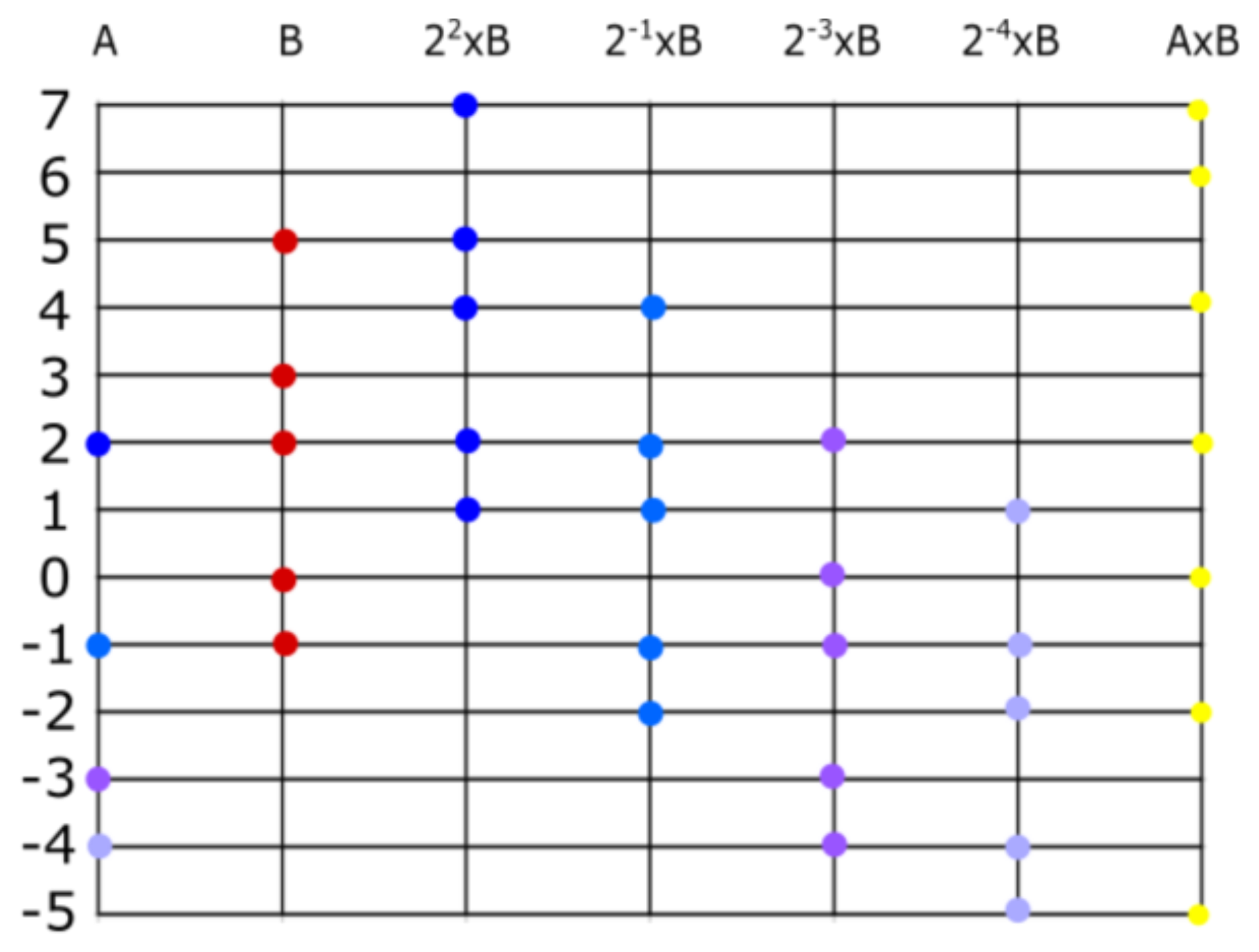
Figure 7 illustrates that the product formula is also valid for negative integers.

3.4. Subtraction

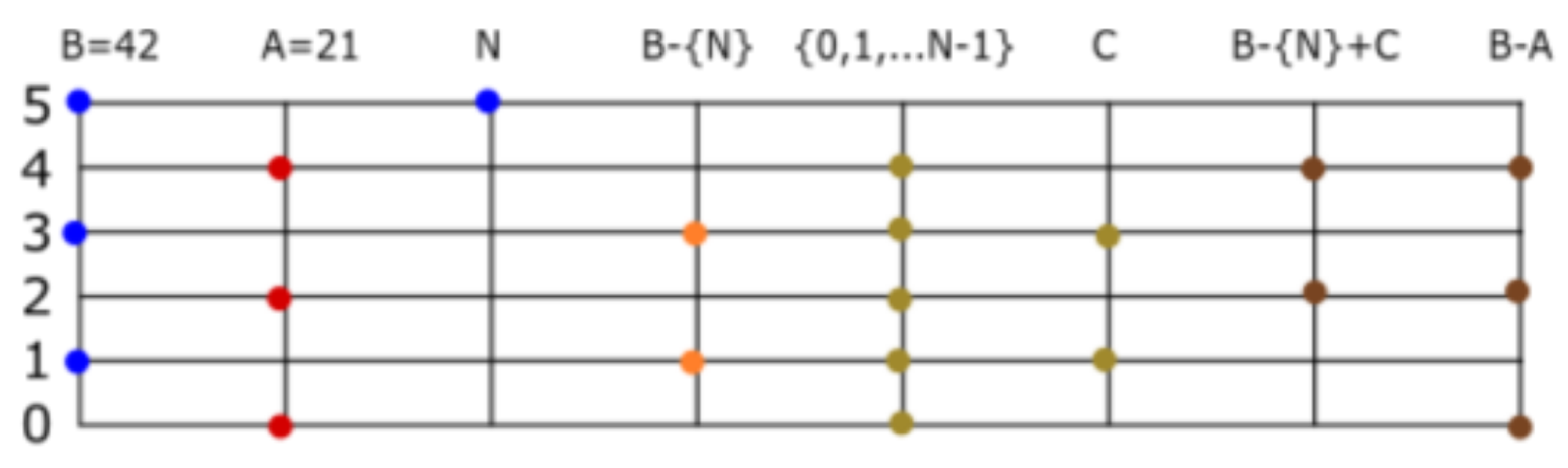
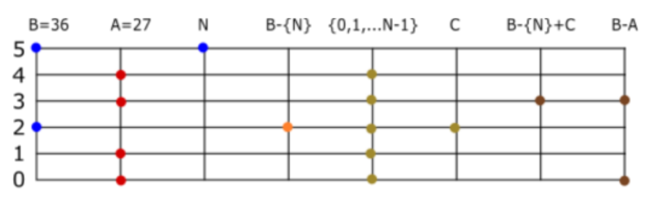
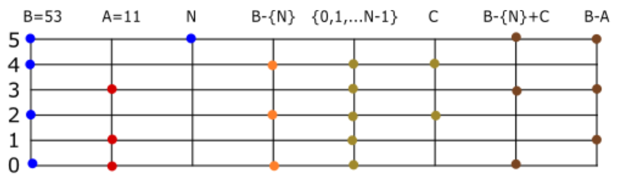
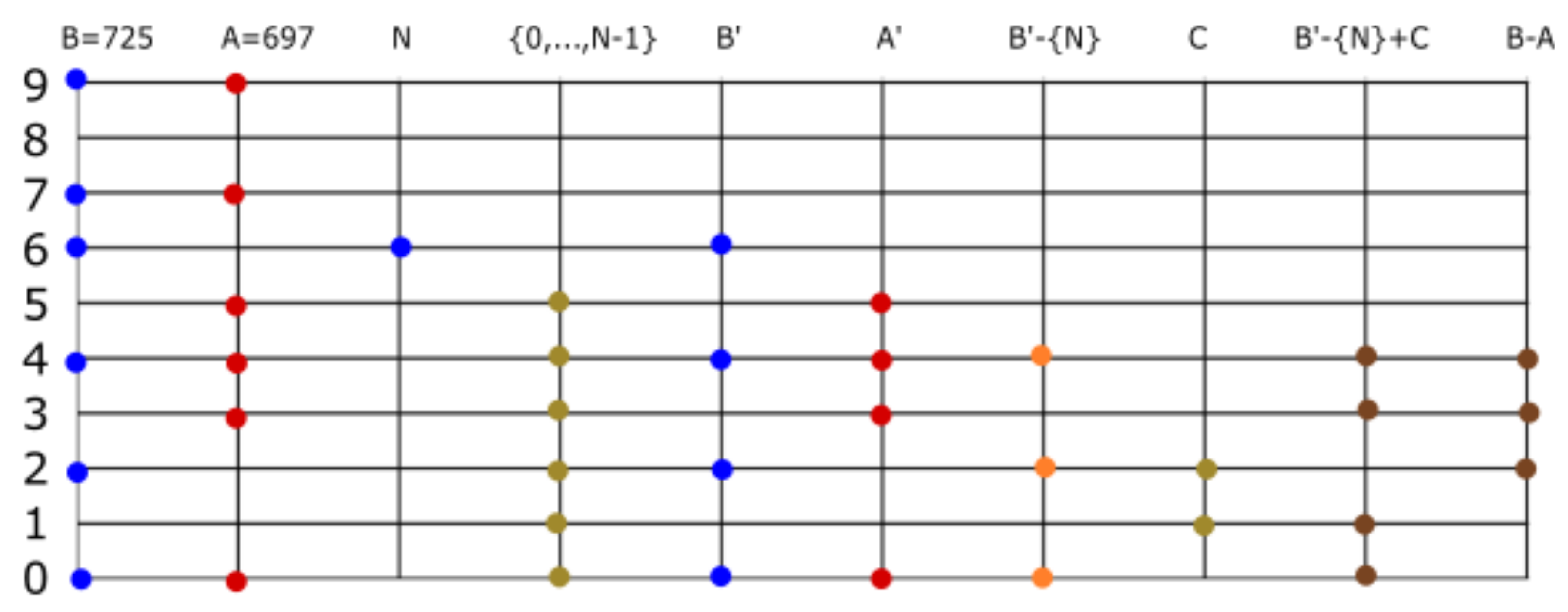
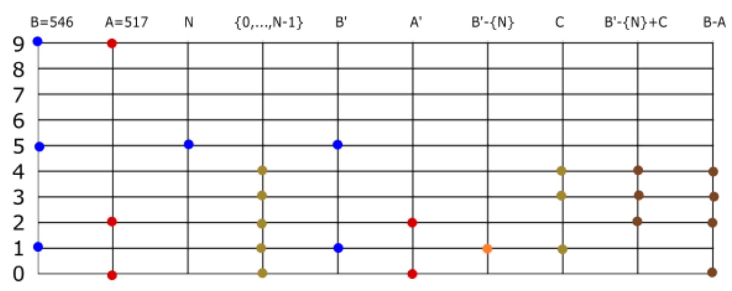
We wish to give forms of inverse operating elements. In this section, we will concentrate on finding an algorithm (and, ultimately, a well defined formula) for subtraction. Before defining the general case, let us begin with two set numbers subject to the relation $A\subset B$. Then, the subtraction is defined by $B\ominus A=B-A$, where $B-A$ is the usual set difference, so that, if we put the two columns side by side, the result $B\ominus A$ is obtained by taking away the particles in the column of B that also appear in A. For example, $45=\{0,2,3,5\}$ and $9=\{0,3\}$ is a subset of 45, so that we can easily find $45-9=\{0,2,3,5\}-\{0,3\}=\{2,5\}=36$. Now, consider two set numbers $A<B$ such that $\max A<\max B$ (strictly less than). We must use our basic rule of addition, now in reverse order, so that we can take away particles from any level of the column B. Rewriting B, we have

$$\begin{array}{ccc}\hfill B& =& (B-\{k\left\}\right)\oplus \left(\right\{k-1\}\oplus \{k-2\}\oplus \cdots \oplus \{1\}\oplus \{0\}\oplus \{0\left\}\right)\hfill \end{array}$$

(1)

for any set number B and any $k\in B$. To find $B\ominus A$ such that $A\oplus (B\ominus A)=B$, we use (1):

$$\begin{array}{ccc}\hfill B\ominus A& =& \left[\right(B-\left\{N\right\})\oplus (\{N-1\}\oplus \{N-2\}\oplus \cdots \oplus \left\{1\right\}\oplus \left\{0\right\}\oplus \left\{0\right\}\left)\right]\ominus A,\hfill \end{array}$$

where $N=\max B$. We know $A\subseteq {\left\{i\right\}}_{i=0}^{N-1}=\{0,1,2,\dots ,N-1\}$. Thus,

$$\begin{array}{ccc}\hfill B\ominus A& =& (B-\{N\left\}\right)\oplus C\oplus \left\{0\right\},\hfill \end{array}$$

(2)

where $C(N,A)=\{0,1,2,\dots ,N-1\}-A$. To find 42-21, we make $B\ominus A=\{1,3,5\}\ominus \{0,2,4\}=\left(\right\{1,3,5\}-\{5\left\}\right)\oplus \left(\right\{0,1,2,3,4\}-A)\oplus \left\{0\right\}=\{1,3\}\oplus \{1,3\}\oplus \left\{0\right\}=\{0,2,4\}$ (see Figure 8, Figure 9 and Figure 10).

Let $A<B$ be two set numbers (with no additional restriction), and let $N_0=\max (A▵B)\in B$. We observe $B\ominus A=B^{\prime }\ominus A^{\prime }$ where $A^{\prime }=A\cap \{0,1,\dots ,N_0\}$ and $B^{\prime }=B\cap \{0,1,\dots ,N_0\}$. The subtraction $B\ominus A$ is treated as in the last paragraph, $\max A^{\prime }<N_0=\max B^{\prime }$. This defines subtraction in the most general case (Figure 11, Figure 12 and Figure 13).

4. Continuum

We will investigate if elements of $Cof\left(\mathbb{N}\right)$ can be multiplied by some set number (outside of the cofinite topology) to obtain $\left\{0\right\}$; it is easy to see $\left\{0\right\}<A\odot B$ if $A,B\in Cof\left(\mathbb{N}\right)$. We include sets that represent reciprocals of natural numbers, by extending our definitions to sets of negative integers. The definitions of order and operation remain the same. Every element of $2^{-\mathbb{N}}$ is smaller than every element of $Cof\left(\mathbb{N}\right)$. We will prove that, for every $X\in Cof\left(\mathbb{N}\right)$, there exists $\frac{1}{X}\in 2^{-\mathbb{N}}$ such that $\frac{1}{X}\odot X=-\mathbb{N}=\left\{0\right\}$. In this section, we prove that the continuum $[0,1]$ is isomorphic to $2^{-\mathbb{N}}$. First, we prove that every subset of $2^{-\mathbb{N}}$ has supremum and infimum. In particular, $\sup \left(2^{-\mathbb{N}}\right)=-\mathbb{N}<\left\{0\right\}$, and $\left\{0\right\}$ is the smallest set number larger than $-\mathbb{N}$. We define $\left\{0\right\}=-\mathbb{N}$ without fear of contradiction. This translates to ${\sum }_{i=-1}^{-\infty }{2}^i=2^0(=1)$. In general, ${\sum }_{i<k}{2}^i=2^k$, or equivalently, $\left\{k\right\}={\left\{i\right\}}_{i<k}$, for any integer k. This means a bounded (above and below) subset of $\mathbb{Z}$ has two representations. After describing the unit interval, we prove ${\mathbb{Z}}^{-}\cong {\mathbb{R}}^{+}$. If $x\in {\mathbb{R}}^{+}$ and $X\in {\mathbb{Z}}^{-}$ is its corresponding set number, the integer part of x is $(X\cap \mathbb{N})\in Cof\left(\mathbb{N}\right)$, and its fractional part is $(X\cap -\mathbb{N})\in 2^{-\mathbb{N}}$.

4.1. $[0,1]\cong 2^{-\mathbb{N}}$

Supremum and Infimum. We define a supremum function for $2^{-\mathbb{N}}$. The order is defined as before, two sets relate $A<B$ if and only if $\max (A▵B)\in B$. Let $\mathbb{X}\subseteq 2^{-\mathbb{N}}$, so that $A\subseteq -\mathbb{N}$ for every $A\in \mathbb{X}$. The well ordering principle implies the existence of $x_1:=\max \bigcup \mathbb{X}$. Define ${\mathbb{Y}}_1:=\{A\in \mathbb{X}|x_1\in A\}$, and $X_1:=(\bigcup {\mathbb{Y}}_1)-\left\{x_1\right\}$, and $x_2:=\max \left(X_1\right)<x_1$. Then, define ${\mathbb{Y}}_2:=\{A\in {\mathbb{Y}}_1|x_2\in A\}$, and $X_2:=(\bigcup {\mathbb{Y}}_2)-\{x_1,x_2\}$, and $x_3:=\max \left(X_2\right)$. Continue in this manner, so that $x_{n+1}:=\max \left(X_n\right)$, where $X_n:=\bigcup {\mathbb{Y}}_n-{\left\{x_i\right\}}_{i=1}^n$ and ${\mathbb{Y}}_n:=\{A\in {\mathbb{Y}}_{n-1}|x_n\in A\}$. In denumerable steps, we have determined a unique set of integers $x_1>x_2>x_3>\cdots$. Define $\sup \mathbb{X}={\left\{x_i\right\}}_i$, which is, by construction, the smallest set number greater than every set in $\mathbb{X}$ (Figure 14).

$2^{2^{-\mathbb{N}}}$ represents the power set, of the power set of $-\mathbb{N}$. The supremum function is a function of the form $\sup :2^{2^{-\mathbb{N}}}\to 2^{-\mathbb{N}}$. If $\sup \left(\mathbb{X}\right)\in \mathbb{X}$, we say $\sup \left(\mathbb{X}\right)=\max \left(\mathbb{X}\right)$. In particular, this is true if $\mathbb{X}$ is finite. There is also an infimum function of the form $\inf :2^{2^{-\mathbb{N}}}\to 2^{-\mathbb{N}}$, where the image of the family is its greatest lower bound. Given a family $\mathbb{X}\subseteq 2^{-\mathbb{N}}$, define ${\mathbb{X}}_{\ast }$ as the family of set numbers that are smaller than or equal to all the elements of $\mathbb{X}$. In other words, $X\subseteq -\mathbb{N}$ is in ${\mathbb{X}}_{\ast }$ if and only if $X<A$, for all $A\in \mathbb{X}$. Then, ${\mathbb{X}}_{\ast }\ne \varnothing$ because $\varnothing \in {\mathbb{X}}_{\ast }$, so that we can define $\inf \left(\mathbb{X}\right)=\sup \left({\mathbb{X}}_{\ast }\right)$. If ${\mathbb{X}}_{\ast }=\{\varnothing \}$, then $\inf \left(\mathbb{X}\right)=\varnothing$. In particular, this implies $\inf [0,1]=0$. To calculate the infimum, find the largest integer $x_1$ such that $\left\{x_1\right\}<X$, for all $X\in \mathbb{X}$. If there is no such integer (the elements of $\bigcup \mathbb{X}$ are arbitrarily small) define $\inf \left(\mathbb{X}\right)=\varnothing$. If $x_1$ exists and $\left\{x_1\right\}\in \mathbb{X}$, then $\inf \left(\mathbb{X}\right)=\left\{x_1\right\}$. If $x_1$ exists and $\left\{x_1\right\}\notin \mathbb{X}$, then we compare $\{x_1,x_1-1\}$ with the elements of X. If $\{x_1,x_1-1\}\in \mathbb{X}$, then $\inf \left(\mathbb{X}\right)=\{x_1,x_1-1\}$. If $\{x_1,x_1-1\}<X$ for every $X\in X$, then $x_2:=x_1-1\in \inf \left(\mathbb{X}\right)$. The last possible case is $\{x_1,x_1-1\}>X$ for some $X\in \mathbb{X}$, so that $x_1-1\notin \inf \left(\mathbb{X}\right)$, and we would then have to verify if $x_1-2\in \inf \left(\mathbb{X}\right)$. This process ends in denumerable steps, with a set $\inf \left(\mathbb{X}\right)={\left\{x_i\right\}}_i\subseteq -\mathbb{N}$.

Reciprocals. If we want to multiply $A\subset \mathbb{N}$ by $B\subseteq -\mathbb{N}$, we proceed as before. The definition is the same. Refer to Figure 7. The unit of product, which should be $\left\{0\right\}$, which is a bounded subset of $\mathbb{Z}$ and therefore has a second representation, which is $-\mathbb{N}$. We use this representation to provide a well-defined algorithm for finding the reciprocal of a natural number. To find the reciprocal of $137=\{0,3,7\}$, we seek out a set number $\frac{1}{N}=\{x_1,x_2,\dots \}\subset -\mathbb{N}$ such that

$$\begin{array}{c}\hfill -\mathbb{N}=\{x_1+0,x_2+0,\dots \}\oplus \{x_1+3,x_2+3,\dots \}\oplus \{x_1+7,x_2+7,\dots \}.\end{array}$$

If we propose $\frac{1}{N}=\{-7\},$ we find we “go over” because:

$$\begin{array}{ccc}\hfill \{0,3,7\}\odot \{-7\}& =& \{-7+0\}\oplus \{-7+3\}\oplus \{-7+7\}=\{-7,-4,0\}>-\mathbb{N}.\hfill \end{array}$$

Now, we try $\frac{1}{N}=\{-8\}$ and we see that we do not go over:

$$\begin{array}{c}\hfill \{0,3,7\}\odot \{-8\}=\{-8+0\}\oplus \{-8+3\}\oplus \{-8+7\}=\{-8,-5,-1\}<-\mathbb{N}.\end{array}$$

(3)

Naturally, proceed to approximate $\frac{1}{N}=\{-8,-9\}$ and find

$$\begin{array}{c}\hfill \{0,3,7\}\odot \{-8,-9\}=\{-1,-2,-5,-6,-8,-9\}<-\mathbb{N}.\end{array}$$

The reader can easily verify $\{0,3,7\}\odot \{-8,-9,-10\}=\{-1,-2,-3,-5,-6,-7,-8,-9,-10\}$. It is equally easy to prove $\{0,3,7\}\odot \{-8,-9,-10,-11\}>-\mathbb{N}$. Continue and verify Figure 15:

$$\begin{array}{ccc}\hfill \{0,3,7\}\odot \{-8,-9,-10,-12\}& =& \{-1,-2,-3,-4,-5,-10,-12\}<-\mathbb{N}.\hfill \end{array}$$

Let us describe the procedure for finding the reciprocal of a set number $N=\{x_1,x_2,\dots ,x_n\}\subset \mathbb{N}$, with $x_1>x_2>\cdots >x_n$. We wish to find a set number $\frac{1}{N}\subset -\mathbb{N}$ such that $N\odot \frac{1}{N}=-\mathbb{N}$. The reciprocal $\frac{1}{N}=\{y_1,y_2,\dots \}\subset -\mathbb{N}$ will be found in denumerable steps, as follows. First, make $y_1=-(x_1+1)$ so that

$$N\odot \{-(x_1+1)\}=\{x_1-(x_1+1),x_2-(x_1+1),\dots ,x_n-(x_1+1)\}=\{-1,x_2-(x_1+1),\dots ,x_n-(x_1+1)\}.$$

Next, find the largest negative integer $y_2$ such that

$$\{-1,x_2-(x_1+1),\dots ,x_n-(x_1+1)\}\oplus \{x_1+y_2,x_2+y_2,\dots ,x_n+y_2\}<-\mathbb{N}.$$

We know that there is at least one negative integer that satisifes this inequality. By the well ordering principle, we can find the maximum of such a set of solutions. This maximum is our integer $y_2$. The finitude of $\#\left(N\right)$ plays a fundamental role in allowing us to guarantee such $y_2$ exists. Now, to find $y_3$, we look for the largest negative integer such that

$$(\{-1,x_2-(x_1+1),\dots ,x_n-(x_1+1)\}\oplus \{x_1+y_2,x_2+y_2,\dots ,x_n+y_2\})\oplus \{x_1+y_3,x_2+y_3,\dots ,x_n+y_3\}<-\mathbb{N}.$$

If we continue in this manner, we have well defined $\frac{1}{N}$.

4.2. ${\mathbb{R}}^{+}\cong {\mathbb{Z}}^{-}$

Topology of Bounded Subsets of $\mathbb{Z}$. A set $X\in {\mathbb{Z}}^{-}$ will correspond to a unique number in ${\mathbb{R}}^{+}$. We do not need to make any modifications to the basic rules and relations of order and operation already used. We extend the same relations to the closed sets of the topology ${\mathbb{Z}}^{-}$. For example, given a binary representation ${110101.00101}_1$, the set number is $\{5,4,2,0,-3,-5\}$.

The positive real line is constructed by piecing together copies of $[0,1]$. Let $X\subset -\mathbb{N}$ be the corresponding set number to $x\in [0,1)$, so that $x={\sum }_{i\in X}{2}^i$. Then, $X\cup \left\{0\right\}$ is the set number corresponding to $1+x=2^0+{\sum }_{i\in X}{2}^i$. More generally, let $N\subset \mathbb{N}$ be the set number corresponding to a natural number $n\in \mathbb{N}$; this means $n={\sum }_{i\in N}{2}^i$. Now, we have $n+x={\sum }_{i\in N}{2}^i+{\sum }_{i\in X}{2}^i={\sum }_{i\in (X\cup N)}{2}^i$. We can summarize our work as follows:

• $\mathbb{N}\cong Cof\left(\mathbb{N}\right)$ where the cofinite topology uses the order and operations of set numbers.
• $[0,1]\cong 2^{-\mathbb{N}}$, with $\varnothing =0$ and $-\mathbb{N}=1$, and the same definitions for set order and operations.
• The continuum of non-negative real numbers is built as a natural generalization of both $Cof\left(\mathbb{N}\right)$ and $2^{-\mathbb{N}}$. We piece together $[0,1],[1,2],[2,3],\dots$, into a single continuum ${\mathbb{R}}^{+}$. This is done by considering the upper bounded sets of $\mathbb{Z}$ and a proper extension of the set number relations.

Let us generalize the previous methods into a single structure isomorphic to ${\mathbb{R}}^{+}$.

Supremum. In the previous sub section, we provided a well defined algorithm for finding the supremum of a family $\mathbb{X}\subseteq [0,1]$, where the elements of $\mathbb{X}$ are arbitrary subsets of $-\mathbb{N}$. Now, we generalize this process to define the supremum of a bounded set of positive real numbers.

Let $\mathbb{X}$ be a bounded set of objects in ${\mathbb{Z}}^{-}$, then $\max \bigcup \mathbb{X}$ exists. In other words, if there exists $A\in {\mathbb{Z}}^{-}$ such that $X<A$ for every $X\in \mathbb{X}$, then $\max \bigcup \mathbb{X}$ exists. Notice that it is not the same as saying "$\mathbb{X}$ is a set of bounded above subsets of $\mathbb{Z}$". We need to guarantee the existence of $\max \bigcup \mathbb{X}$ in order to find the supremum of $\mathbb{X}$. This is done by asking that $\mathbb{X}$ be bounded above in the order of ${\mathbb{Z}}^{-}$. For example, there is no $\max \bigcup \mathbb{X}$ for

$$\mathbb{X}=\left\{\right\{1,0,-1,-2,\dots \},\{2,1,0,-1,\dots \},\{3,2,1,0,\dots \},\{4,3,2,1,\dots \},\dots \},$$

although $\mathbb{X}\subset {\mathbb{Z}}^{-}$. This is due to the fact that $\mathbb{X}$ is not bounded in the order of set numbers.

Once the reader verifies the existence of $x_1=\max \bigcup \mathbb{X}$, it is easy to follow the same algorithm we provided for finding the supremum of subfamilies of $2^{-\mathbb{N}}$. Let us find the supremum of a finite list of set numbers; obviously, the result should be the maximum of the list. These are $A=\{4,2,1,-1,-3,-5,-7,\dots \}$, $B=\{4,3,-1,-3,-5,-7,\dots \}$, $C=\{4,2,1,0,-2,-4,-6,\dots \}$, $D=\{4,3,0,-2,-4,-6,\dots \}$, $E=\{4,3,0,-1,-2,-4,-6,\dots \}$. We wish to find $\sup \left(\mathbb{X}\right)$, where $\mathbb{X}=\{A,B,C,D,E\}$. First, we find the maximum of $\bigcup \mathbb{X}$; the maximum integer that appears in our set numbers is $x_1=4$. Then, we define the family ${\mathbb{Y}}_1\subseteq \mathbb{X}$ of those set numbers that have 4 as an element. In this case $A,B,C,D,E$ all have 4 as element so that ${\mathbb{Y}}_1=\mathbb{X}$. Now, we find the maximum of $X_1=(\bigcup {\mathbb{Y}}_1)-\left\{x_1\right\}$; the second largest number that appears in the family ${\mathbb{Y}}_1$ is $x_2=3$. Now, ${\mathbb{Y}}_2=\{B,D,E\}$ because these are the only set numbers of ${\mathbb{Y}}_1$ that contain $x_2=3$. The maximum of $X_2=(\bigcup {\mathbb{Y}}_2)-\{x_1,x_2\}$ is the third largest number that appears in the family ${\mathbb{Y}}_2$. It is $x_3=0$, and the only elements of ${\mathbb{Y}}_2$ that contain 0 are $D,E$ so that ${\mathbb{Y}}_3=\{D,E\}$. We find $x_4=\max ((\bigcup {\mathbb{Y}}_3)-\{4,3,0\})=-1$ and $-1$ is not an element of D, but it is an element of E; then, ${\mathbb{Y}}_4=\left\{E\right\}$. We find $x_5=-2$, $x_6=-4$, $x_7=-6$, …. We conclude $\sup \left(\mathbb{X}\right)=\max \left(\mathbb{X}\right)=E$.

Division. We now describe division and rational numbers. Let us find the rational representation of the set number $\{5,0,-2,-4,-5\}=33.34375$. If we apply $s^5$ to the set number, the result is $\{10,5,3,1,0\}=1067$. The action of adding 5 to the elements of a set number is equivalent to multiplication by $2^5$. In our example, $\left\{5\right\}\odot \{5,0,-2,-4,-5\}=\{10,5,3,1,0\}$. If $A\in {\mathbb{Z}}^{-}$, we define $\mathbb{A}=\{X\in Cof(\mathbb{N}\left)\right|X\odot A\in Cof\left(\mathbb{N}\right)\}$. If $\mathbb{A}=\varnothing$, we say the set number A is irrational, and if $\mathbb{A}\ne \varnothing$, then A is rational. A fraction representing A is an ordered pair $(M,N)$, where $N\in Cof\left(\mathbb{N}\right)$ is an element of $\mathbb{A}$ and $M=N\odot A$. If A is rational, the well ordering principle implies the existence of $\min \left(\mathbb{A}\right)$, and the corresponding fraction is said to be the irreducible fraction of $\mathbb{A}$. In our example, $\left(\right\{10,5,3,1,0\},\{5\left\}\right)$ is the irreducible fraction of $\{5,0,-2,-4,-5\}$. This can be expressed as $33.34375=\frac{1067}{32}$. Given a finite set number $A\in {\mathbb{Z}}^{-}$, we can give infinite, but equivalent, representations of an irreducible fraction $\frac{m}{n}$.

Consider the inverse problem of finding the set number corresponding to an ordered pair $\frac{m}{n}$. Let $M,N$ be the set numbers corresponding to $m,n$, respectively. Then, $A=M\odot \frac{1}{N}$. Approximate $\frac{51}{137}$ by multiplying $\frac{1}{137}\approx \{-8,-9,-10,-12\}$ with $51=\{5,4,1,0\}$, to obtain $0.361083984375=\{-2,-4,-5,-6,-10,-11,-12\}$. For more precision, we must give a better approximation to the number $\frac{1}{137}$. For example, $\frac{1}{137}\approx \{-8,-9,-10,-12,-13,-14,-17\}$. Approximate $\frac{137}{51}$ by two methods. Find the product of $1/51$ and $\{7,2,0\}$; we have to find the set number corresponding to $\frac{1}{51}$. The second method consists of approximating B such that $\{-2,-4,-5,-6,-10,-11,-12\}\odot B=-\mathbb{N}$.

We can fully describe the set of rational and irrational numbers. Let $A\in {\mathbb{Z}}^{-}$ be a set number with $A\cap -\mathbb{N}$ finite. Then, A is a rational number. If $A\cap -\mathbb{N}$ is infinite, then A is irrational, with one crucial exception. If the set $A\cap -\mathbb{N}$ is infinite and periodic, then $\mathbb{A}\ne \varnothing$ and A is rational.

Sum and Product of Infinite Sets. We must define the set number sum of two sets $A,B\in {\mathbb{Z}}^{-}$ each with perhaps infinite elements. A, is the set of integers $a_1>a_2>a_3>\cdots$, and B the set of integers $b_1>b_2>b_3>\cdots$. Define $A_n={\left\{a_i\right\}}_{i=1}^n$, and in a similar manner $B_m={\left\{b_m\right\}}_{j=1}^m$. The sum is defined as $A\oplus B:={\sup }_{n,m}(A_n\oplus B_m)$ for all $n,m\in N$. The reader can define the multiplication of two infinite set numbers.

Powers. To take powers of set numbers $A^B$, we start by defining $A^B$, where $A,B\subset \mathbb{N}$. In this case, $X=A^B$ is the result of carrying out successive products of set numbers. The empty set is representing the integer 0, so we define the power $A^{\varnothing }=\left\{0\right\}$. We define the power $A^{\left\{0\right\}}=A$ because $\left\{0\right\}=1$. With this, we are able to give a recursive formula $A^B=A\odot A^{B\ominus \left\{0\right\}}$. To find the power of ${127}^4={\{0,1,2,3,4,5,6\}}^{\left\{2\right\}},$ we first reduce the expression. We know $A^{\left\{2\right\}}=A\odot A^{\left\{2\right\}\ominus \left\{0\right\}}$. We know, from the subtraction of set numbers, that $\left\{2\right\}\ominus \left\{0\right\}=\{0,1\}$, then $A^{\left\{2\right\}}=A\odot A^{\{0,1\}}$. Then, we find $A^{\{0,1\}}=A\odot A^{\{0,1\}\ominus \left\{0\right\}}=A\odot A^{\left\{1\right\}}=A\odot (A\odot A^{\left\{1\right\}\ominus \left\{0\right\}})=A\odot (A\odot A)$. Finally, $A^{\left\{2\right\}}=A\odot (A\odot (A\odot A))$, as we expect since $\left\{2\right\}=4$.

$$\begin{array}{ccc}\hfill 127·127& =& \{0,1,2,3,4,5,6\}\odot \{0,1,2,3,4,5,6\}\hfill \\ \hfill & =& \underset{a\in 127}{⨁}{\{a+b\}}_{b\in 127}\hfill \\ \hfill & =& \{0,8,9,10,11,12,13\}.\hfill \end{array}$$

Now, we take $\{0,8,9,10,11,12,13\}$ as base and use $\{0,1,2,3,4,5,6\}$ as pivot so that

$$\begin{array}{ccc}\hfill {127}^3& =& \{0,1,2,3,4,5,6\}\odot \{0,8,9,10,11,12,13\}\hfill \\ \hfill & =& \underset{a\in 127}{⨁}{\{a+b\}}_{b\in 16,129}\hfill \\ \hfill & =& \{0,1,2,3,4,5,6,8,14,16,17,18,19,20\}.\hfill \end{array}$$

The reader can verify the final result, carrying out the following addition of set numbers.

$$\begin{array}{ccc}\hfill {127}^4& =& \{0,1,2,3,4,5,6\}\odot \{0,1,2,3,4,5,6,8,14,16,17,18,19,20\}\hfill \\ \hfill & =& \underset{a\in 127}{⨁}{\{a+b\}}_{b\in {127}^3}.\hfill \end{array}$$

If the set number $A\in {\mathbb{Z}}^{-}$ has infinite elements $a_1>a_2>a_3>\cdots$, we define the power $A^B=\underset{n}{\sup }{A}_n^B$, where $A_n={\left\{a_i\right\}}_{i=1}^n$. There are two cases: (1) if $A<\left\{0\right\}$, then $A^X$ is a decreasing function, and (2) if $A>\left\{0\right\}$, then $A^X$ is an increasing function. Proving this is not difficult but requires some labor. Before proving it for arbitrary set numbers X, it has to be proven for $X\in Cof\left(\mathbb{N}\right)$ and $1/X$. Taking negative powers is notation for the reciprocal of a power; $A^{-3}:=1/A^3$ which corresponds to the set number $1/A^{\{0,1\}}$. In addition, ${\left\{0\right\}}^X=\left\{0\right\}$, for every set number $X\in Cof\left(\mathbb{N}\right)$.

Roots. The process of finding a root is finding a reciprocal power, that is to say $A^{\frac{1}{B}}$, for some set $B\in Cof\left(\mathbb{N}\right)$. To find $X=A^{\frac{1}{B}}$, we must find a set $X\in {\mathbb{Z}}^{-}$ such that $X^B=A$. The set $P(A,B)$ of all set numbers X such that $X^B<A$ is bounded above. Define $A^{\frac{1}{B}}=\sup P(A,B)$. We have three cases; $A>\left\{0\right\}$, $A=\left\{0\right\}$, and $A<\left\{0\right\}$. In the first case, $A^{\frac{1}{B}}<A$, while in the last case $A^{\frac{1}{B}}>A$. The roots of $\left\{0\right\}$ are ${\left\{0\right\}}^{\frac{1}{B}}=\left\{0\right\}$, for every $B\in Cof\left(\mathbb{N}\right)$. We give an example, $3^{1/4}={\{0,1\}}^{1/\left\{2\right\}}$. The fourth power of $\{0,-1\}$ is greater than $\{0,1\}$. We find that ${\{0,-2\}}^4<\{0,1\}$, and $\{0,-2,-3\}>\{0,1\}$. Then, we find $\{0,-2,-4\}<\{0,1\}$. We continue in this manner, with trial and error; finding the fourth power of sets such that the fourth power is less than {0,1}. We are finding a number whose fourth power is equal to the natural number $3=\{0,1\}$.

To take rational powers $A^B$, with B a rational number, we find the irreducible fraction $B=\frac{m}{n}$. Now, $A^B={\left(A^m\right)}^{\frac{1}{n}}$ is well defined because it can be proven ${\left(A^m\right)}^{\frac{1}{n}}={\left(A^{\frac{1}{n}}\right)}^m$. Consider next the general case where B is not rational. Let $A,B\in {\mathbb{Z}}^{-}$ arbitrary set numbers, and $b_1>b_2>b_3\cdots$ are the elements of B. Let $B_k={\left\{b_i\right\}}_{i=1}^k$; then, to every $B_k$, there corresponds an irreducible fraction $Q_k=\frac{m_k}{n_k}$. We define $A^B=\underset{k}{\sup }{A}^{Q_k}$. Of course, for this definition to be justified, we have to prove the set ${\left\{A^{Q_k}\right\}}_{k=1}^{\infty }$ is bounded above. Hint: prove the power function $A^X$ is increasing with X, then it suffices to show ${\left\{B_k\right\}}_{k=1}^{\infty }$ is bounded above; $\{b_1+1\}>B_k$ for all k.

Logarithms. In the last section, we extended the definition of powers to include rational numbers and, finally, irrational powers as well. Now, we explore the inverse function. To find $X={\log }_{B}A$, we find a set number X such that $B^X=A$. It is not difficult to prove the following statements.

If $\left\{0\right\}<A<B$, then there exists a positive real number $\left\{0\right\}>X\in {\mathbb{Z}}^{-}$ such that $B^X=A$. If $\left\{0\right\}<B<A$, then there exists a positive real number $\left\{0\right\}<X\in {\mathbb{Z}}^{-}$ such that $B^X=A$. If $B<A<\left\{0\right\}$ then $X<\left\{0\right\}$. If $A<B<\left\{0\right\},$ then $\left\{0\right\}<X$.

Let us calculate $lo{g}_{2.5}3.125$ which is the logarithm base $2.5$ of $3.125$. The numerical value is $\approx 1.24353$. We have $B=\{-1,1\}$ and $A=\{-3,0,1\}$, and we wish to find a fraction $X=\frac{m}{m}$ such that ${\left(B^m\right)}^{\frac{1}{n}}=A$. Begin by calculating ${2.5}^2$, to see if we go over $3.125$ or not. Multiplying $\{-1,1\}$ by itself is equal to the set sum $\{-2,0\}\oplus \{0,2\}=\{-2,1,2\}$. The result is a set number larger than $\{-3,0,1\}$. Next, we try $\left\{0\right\}<Y<\left\{1\right\}$ because ${2.5}^{\left\{0\right\}}=2.5$. Use $\{0,-1\}=\frac{3}{2}$; first, we find the third power of $2.5$ and then we find the square root.

$$\begin{array}{ccc}\hfill {2.5}^3& =& {2.5}^2·2.5\hfill \\ \hfill & =& \{-2,1,2\}\odot \{-1,1\}\hfill \\ \hfill & =& \{-3,-1,0,1,2,3\}.\hfill \end{array}$$

Next, we find the square root of $\{-3,-1,0,1,2,3\}$. $\{-1,0,1\}\subset {\{-3,-1,0,1,2,3\}}^{\frac{1}{2}}$, so that ${2.5}^{\frac{3}{2}}>\{-3,0,1\}$. Our next candidate for Y is $\{0,-2,\}=\frac{5}{4}$. The fifth power of $2.5$ is equal to ${\{-1,1\}}^5=\{-5,-3-1,0,5,6\}$. Searching the fourth root of this last set number gives $\{-6,-3,0,1\}\subset {\{-5,-3-1,0,5,6\}}^{\frac{1}{4}}$. Our next approximation for Y is $\{-3,0\}=\frac{9}{8}$. We find ${\{-1,1\}}^{\{-3,0\}}<\{-3,0,1\}$. Then, we find ${\{-1,1\}}^{\{-4,-3,0\}}<\{-3,0,1\}$ and ${\{-1,1\}}^{\{-5,-4,-3,0\}}<\{-3,0,1\}$ so that we approximate ${\log }_{2.5}3.125\approx 1.21875$. Taking another step gives ${\log }_{2.5}3.125\approx \{-6,-5,-4,-3,0\}=1.234375$.

The logarithm base B of A can be approximated by rational numbers, as follows. Find two set numbers $M,N\in Cof\left(\mathbb{N}\right)$ such that $\frac{A^N}{B^M}\approx 1$. The rational approximation is $lo{g}_{B}A\approx \frac{M}{N}$.

Properties of Operation. The axiomatic properties of the field of real numbers hold, taking into account that we have not yet described negative real numbers. The identity for addition is ∅, while the identity for product is $\left\{0\right\}$. The commutative property of addition is trivial because of the commutative properties of ▵ and ∩. It is not easy to give a direct proof of the associative property for set number addition. We first have to show $\left\{n\right\}\oplus (A\oplus \{m\left\}\right)=\left(\right\{n\}\oplus A)\oplus \left\{m\right\}$, for any singletons $\left\{n\right\},\left\{m\right\}\subset \mathbb{Z}$. Let $N=\{x_1,x_2,\dots ,x_n\}$, $M=\{y_{,}{1}_2,\dots ,y_m\}$ and $A=\{a_1,a_2,\dots ,a_p\}$ three finite subsets of $\mathbb{Z}$. The sum of these can be written

$$\begin{array}{ccc}\hfill N\oplus (A\oplus M)& =& (\left\{x_1\right\}\oplus \left\{x_2\right\}\cdots \left\{x_n\right\})\oplus [A\oplus (\left\{y_1\right\}\oplus \left\{y_2\right\}\cdots \left\{y_m\right\})]\hfill \\ \hfill & =& \left\{x_1\right\}\oplus (\left\{x_2\right\}\oplus \cdots \oplus (\left\{x_n\right\}\oplus (((A\oplus \left\{y_1\right\})\oplus \left\{y_2\right\})\oplus \cdots \oplus \left\{y_m\right\}))).\hfill \end{array}$$

From this, it is possible to prove $N\oplus (A\oplus M)=(N\oplus A)\oplus M$. The commutative and associative properties of product are much more difficult to prove. The same can be said of distributive property; the proof does not seem to be trivial. It is easy, however, to prove that $\left\{n\right\}$ commutes with any set number X, under product. Then, distributivity implies commutativity of product in $Cof\left(\mathbb{N}\right)$.

5. Construction of $\mathbb{R}$

We provide two constructions of the real number system. The first method consists of fitting all the real numbers into the unit interval; we use this to define an explicit isomorphism between the set of real numbers and $2^{-\mathbb{N}}\cong [0,1]$. We want to build the structure of real numbers which is a union of intervals $\mathbb{R}=(I_1\cup I_2\cup \cdots )\cup (-I_1\cup -I_2\cup \cdots )$, where $I_k=[k-1,k)$ and $-I_k=(-k,-k+1]$. That is to say, $\mathbb{R}=\cdots (-2,-1]\cup (-1,0]\cup [0,1)\cup [1,2)\cup \cdots$. The intervals $-I_k$ will be the intervals $(1/4,1/2],(1/8,1/4],(1/16,1/8]\cdots \subset [0,1/2]$, while the $I_k$ will be $[1/2,3/4),[3/4,7/8),[15/16,7/8),\cdots \subset [1/2,1]$. The number $0\in \mathbb{R}$ is identified with $1/2$ in the unit interval, and $+\infty ,-\infty$ are 0 and 1, respectively. See Figure 16.

Our second method consists of building the real numbers as a space of functions. Positive real numbers are functions $+x$ so that $+x\left(a\right)=a+x$. The negative real numbers are their inverse functions, and 0 is the identity function $Id:{\mathbb{R}}^{+}\to {\mathbb{R}}^{+}$.

Unit Interval. The real numbers of $I_1$ are set numbers of the form $\{-1,x_1,x_2,x_3,\dots \}$, with $x_i\le -3$. Next, we define $I_2$ as the collection of set numbers of the form $\{-1,-2,x_1,x_2,x_3,\dots \}$, with $x_i\le -4$. The interval $I_3$ is the collection of set numbers $\{-1,-2,-3,x_1,x_2,x_3,\dots \}$, with $x_i\le -5$. The negative interval $-I_1=[-1,0)$ is the collection of set numbers of the form $\{-2,x_1,x_2,x_3,\dots \}$ with $x_i\le -3$. The real number $-1\in \mathbb{R}$ is identified with $\frac{1}{4}=\{-2\}$, and $-\frac{1}{2}\in \mathbb{R}$ is the set number $\{-2,-3\}$. The interval $-I_2$ is defined as the family of sets $\{-3,x_1,x_2,x_3,\dots \}$, with $x_i\le -4$

There are two types of set numbers: 1) If $-1\in X$, then we say X is a positive set number 2). If $-1\notin X$, then X is a negative set number. Positive set numbers are of the form $\{-1,-2,-3,\dots ,-n,x_1,x_2,x_3,\dots \}$ with $-2\ge -n-1>x_1>x_2>x_3>\cdots$, while negative numbers are sets of the form $\{-n,x_1,x_2,x_3,\dots \}$ with $-1>-n>x_1>x_2>x_3>\cdots$. Let $X\in {\mathbb{Z}}^{-}$ a set number with $\{a_1,a_2,a_3,\dots \}=X\cap -\mathbb{N}$ and a finite set of natural numbers $N=X\cap \mathbb{N}$. Define $n={\sum }_{i\in N}{2}^i$, then $X^{\prime }=\{-1,-2,-3,\dots ,-n,a_1-(n+1),a_2-(n+1),a_3-(n+1),\dots \}$ is the new representation of the set number X. The set number X can also be identified with another set we will call the negative of $X^{\prime }$, and it is $-X^{\prime }=\{-(n+1),a_1-(n+1),a_2-(n+1),a_3-(n+1),\dots \}$.

Let $X=7.28125=\{-5,-2,0,1,2\}$, then the new representation is

$$X^{\prime }=\{-1,-2,-3,-4,-5,-6,-7,-8,-2-(8+1),-5-(8+1)\}=\{-1,-2,-3,-4,-5,-6,-7,-8,-11,-14\}$$

because the integer part is 7 and therefore $n=8$. The negative is $-X^{\prime }=\{-9,-2-9,-5-9\}=\{-9,-11,-14\}$. It is left as an exercise to prove every subset of $-\mathbb{N}$ corresponds to a unique real number, and vice versa. We can obviously identify every real number with a unique subset of $\mathbb{N}$, now that we can identify it with a unique subset of $-\mathbb{N}$. The main idea behind this construction is that we use the first n natural numbers of a set number to determine the sign and the integer part.

In this paragraph, we have proven that there is a way of defining an order relation for $2^{\mathbb{N}}$, and that this order is isomorphic to the order of the extender real number line $\mathbb{R}$. The operations can be meticulously defined case by case, but we will not unnecessarily extend our discussion.

Function Space. Our second construction, of negative real numbers, involves inverse functions. Every positive real number $X\in {\mathbb{Z}}^{-}$ can be associated a unique isomorphism $\oplus X:{\mathbb{Z}}^{-}\to {\mathbb{R}}_X$, where ${\mathbb{R}}_X\subset {\mathbb{Z}}^{-}$ is the collection of positive real numbers that are greater than or equal to X. In other words, an isomorphism ${\mathbb{R}}^{+}\to \{\oplus X\}$ is given and $\oplus X:{\mathbb{Z}}^{-}\to {\mathbb{R}}_X$ is the bijection that acts by $\oplus X\left(A\right)=A\oplus X$. Let ${\mathbb{R}}^{\ast }=\{\oplus X\}\cup \left\{{(\oplus X)}^{-1}\right\}\cup \left\{Id\right\}$. We have two classes of functions in ${\mathbb{R}}^{\ast }$, as far as domain and range—the objects we call negative real numbers, and the positive real numbers.

We define an operation for elements of ${\mathbb{R}}^{\ast }$. The operation of two positive real numbers is defined to be the composition $\oplus X\circ \oplus Y:{\mathbb{Z}}^{-}\to {\mathbb{R}}_{X\oplus Y}$, where X and Y are the set numbers corresponding to $\oplus X,\oplus Y$, respectively. It is natural to define the sum of two negative elements, ${(\oplus X)}^{-1},{(\oplus Y)}^{-1}$, by ${(\oplus X)}^{-1}\circ {(\oplus Y)}^{-1}:={(\oplus X\circ \oplus Y)}^{-1}\in {\mathbb{R}}^{\ast }$. Now, we must find a suitable definition for $\oplus X\circ {(\oplus Y)}^{-1}$. If $Y<X$, then we can find the set number $X\ominus Y>0$ and its function $\oplus (X\ominus Y):{\mathbb{Z}}^{-}\to {\mathbb{R}}_{X\ominus Y}\in {\mathbb{R}}^{\ast }$; this function is defined to be the result of $\oplus Y^{-1}\circ \oplus X=\oplus X\circ \oplus Y^{-1}$. If $X<Y$, then define $\oplus Y^{-1}\circ \oplus X=\oplus X\circ \oplus Y^{-1}={(\oplus Y\circ \oplus X^{-1})}^{-1}\in {\mathbb{R}}^{\ast }$. This operation $\circ :{\mathbb{R}}^{\ast }\times {\mathbb{R}}^{\ast }\to {\mathbb{R}}^{\ast }$ is addition of real numbers.

Denote the elements of ${\mathbb{R}}^{\ast }$ with bold letters, $\mathbf{X},\mathbf{Y},\cdots \in {\mathbb{R}}^{\ast }$. We can build an isomorphism $+:{\mathbb{R}}^{\ast }\to {\mathbb{R}}^{\ast \ast }$, where ${\mathbb{R}}^{\ast \ast }$ is a collection of bijections of the form ${\mathbb{R}}^{\ast }\to {\mathbb{R}}^{\ast }$. The isomoprphism $+\mathbf{X}:{\mathbb{R}}^{\ast }\to {\mathbb{R}}^{\ast }$ is defined by $\mathbf{Y}{\mapsto }_{+\mathbf{X}}\mathbf{Y}\circ \mathbf{X}$. The elements of ${\mathbb{R}}^{\ast }$ are functions on ${\mathbb{Z}}^{-}$. The elements of ${\mathbb{R}}^{\ast \ast }$ are bijective functions of the form ${\mathbb{R}}^{\ast }\to {\mathbb{R}}^{\ast }$. In conclusion, $\mathbb{R}\cong {\mathbb{R}}^{\ast }\cong {\mathbb{R}}^{\ast \ast }$, and ${\mathbb{R}}^{\ast \ast }$ gives a complete description of addition for real numbers.

6. Universe of Finite Sets

Previous expositions of axiomatic set theory for analysis begin with a description of the natural numbers in two main forms [7] (pp. 21–22). These are known as Zermelo ordinals, and Neumann ordinals. The first is the set $\{\varnothing ,\{\varnothing \},\{\{\varnothing \}\},\{\left\{\right\{\varnothing \left\}\right\}\},\dots \}$. That is to say, natural numbers have been characterized as $0=\varnothing$, $1=\left\{0\right\}$, $2=\left\{1\right\}$, and in general $n+1:=\left\{n\right\}$ (Zermelo, 1908). The second way, due to von Neumann, is $\mathbb{N}=\{\varnothing ,\{\varnothing \},\{\varnothing ,\{\varnothing \}\},\{\varnothing ,\{\varnothing \},\{\varnothing ,\{\varnothing \left\}\right\}\},\dots \}$ and, in this case, every natural number is the set of its predecessors, so that $x+1:=x\cup \left\{x\right\}$. These constructions assign natural numbers to sets that are obtainable from the empty set in finite steps. However, in both cases, some sets are left out. For example, the sets $\{\varnothing ,\{\{\varnothing \}\left\}\right\}$ and $\{\varnothing ,\{\{\varnothing \},\left\{\right\{\varnothing \left\}\right\}\left\}\right\}$ are not natural numbers in either ordinal family. This is part of Benacerraf’s identification problem.

One of our results is that the set ${\mathbb{U}}_0$, of objects constructed from the empty set with finite steps, is equivalent to $Cof\left(\mathbb{N}\right)$. In this sense, we don’t leave out any sets of ${\mathbb{U}}_0$ when identifying them with natural numbers. Indeed, all elements of ${\mathbb{U}}_0$ represent a unique natural number in $Cof\left(\mathbb{N}\right)$. In defining the structure of $Cof\left(\mathbb{N}\right),$ we defined:

$$\begin{array}{ccc}\hfill 0& =& \varnothing \hfill \\ \hfill 1& =& \left\{0\right\}=\{\varnothing \}\hfill \\ \hfill 2& =& \left\{1\right\}=\left\{\right\{\varnothing \left\}\right\}\hfill \\ \hfill 3& =& \{0,1\}=\{\varnothing ,\{\varnothing \left\}\right\}\hfill \\ \hfill 4& =& \left\{2\right\}=\left\{\right\{\{\varnothing \}\left\}\right\}\hfill \\ \hfill 5& =& \{0,2\}=\{\varnothing ,\{\{\varnothing \}\left\}\right\}\hfill \\ \hfill 6& =& \{1,2\}=\left\{\right\{\varnothing \},\{\{\varnothing \}\left\}\right\}\hfill \\ \hfill 7& =& \{0,1,2\}=\{\varnothing ,\{\varnothing \},\{\{\varnothing \}\left\}\right\}\hfill \\ \hfill 8& =& \left\{3\right\}=\left\{\right\{\varnothing ,\{\varnothing \}\left\}\right\}\hfill \\ \hfill 9& =& \{0,3\}=\{\varnothing ,\{\varnothing ,\{\varnothing \}\left\}\right\}\hfill \\ \hfill ⋮& ⋮\hfill \end{array}$$

Definition 1.

Define a universe of sets ${\mathbb{U}}_0$.

1. 

$\varnothing \in {\mathbb{U}}_0$

2. 

$x_1,x_2,x_3,\dots ,x_n\in {\mathbb{U}}_0$, then $\{x_1,x_2,x_3,\dots ,x_n\}\in {\mathbb{U}}_0$

3. 

${\mathbb{U}}_0$ is the set of objects that satisfy 1. or 2.

Definition 2.

For any $\varnothing \ne X\in {\mathbb{U}}_0$, define $X\oplus \{\varnothing \}=(X▵\{\varnothing \left\}\right)\oplus R$, where $R={\{x\oplus \{\varnothing \}\}}_{x\in (X\cap \{\varnothing \left\}\right)}$. For the empty set, we define $\varnothing \oplus \{\varnothing \}=\{\varnothing \}\oplus \varnothing =\{\varnothing \}$. For any two $A,B\in {\mathbb{U}}_0$, we define the operation $A\oplus B=(A▵B)\oplus {\{x\oplus \{\varnothing \}\}}_{x\in (A\cap B)}$. In particular, define $A\oplus \varnothing =\varnothing \oplus A=A$.

Axiom 1.

Definition 2. Provides a bijection $\oplus \{\varnothing \}:{\mathbb{U}}_0\to ({\mathbb{U}}_0-\{\varnothing \})$ that serves as successor function; the successor of X being $\oplus \{\varnothing \}\left(X\right)=X\oplus \{\varnothing \}$.

The function $\oplus \{\varnothing \}$ is different than $s\left(X\right)$, which added 1 to the elements of X. This function is equivalent to the successor function that defines natural numbers.

Axiom 2.

The definition of $A\oplus B$ defines the operation of addition for natural numbers. We can always find the set $A\oplus B$ in finite steps, and this operation is isomorphic to the usual addition of natural numbers.

Let $x\in \mathbb{N}$ and $X\in Cof\left(\mathbb{N}\right)$ be its set number. It is left as an exercise for the reader to prove $\oplus \{\varnothing \}\left(X\right)$ is the set number corresponding to $x+1$, for every $0\le x\le 8$, and compare the results:

$$\begin{array}{ccc}\hfill \{\varnothing \}\oplus \{\varnothing \}& =& \varnothing \oplus {\left\{s\left(x\right)\right\}}_{x\in \{\varnothing \}}\hfill \\ \hfill & =& {\left\{s\left(x\right)\right\}}_{x\in \{\varnothing \}}\hfill \\ \hfill & =& \left\{s\right(\varnothing \left)\right\}\hfill \\ \hfill & =& \left\{\right\{\varnothing \left\}\right\}\hfill \end{array}$$

$$\begin{array}{ccc}\hfill \left\{\right\{\varnothing \left\}\right\}\oplus \{\varnothing \}& =& \{\varnothing ,\{\varnothing \}\}\oplus {\left\{s\left(x\right)\right\}}_{y\in \varnothing }\hfill \\ \hfill & =& \{\varnothing ,\{\varnothing \left\}\right\}\oplus \varnothing \hfill \\ \hfill & =& \{\varnothing ,\{\varnothing \left\}\right\}\hfill \end{array}$$

$$\begin{array}{ccc}\hfill \{\varnothing ,\{\varnothing \left\}\right\}\oplus \{\varnothing \}& =& \left\{\{\varnothing \}\right\}\oplus {\left\{s\left(x\right)\right\}}_{x\in \{\varnothing \}}\hfill \\ \hfill & =& \left\{\right\{\varnothing \left\}\right\}\oplus \left\{s\right(\varnothing \left)\right\}\hfill \\ \hfill & =& \left\{\right\{\varnothing \left\}\right\}\oplus \left\{\right\{\varnothing \left\}\right\}\hfill \\ \hfill & =& \varnothing \oplus {\left\{s\left(x\right)\right\}}_{x\in \left\{\right\{\varnothing \left\}\right\}}\hfill \\ \hfill & =& \left\{s\right(\{\varnothing \}\left)\right\}\hfill \\ \hfill & =& \left\{\right\{\{\varnothing \}\left\}\right\}.\hfill \end{array}$$

$$\begin{array}{ccc}\hfill \left\{\right\{\{\varnothing \}\left\}\right\}\oplus \{\varnothing \}& =& \{\varnothing ,\left\{\{\varnothing \}\right\}\}\oplus {\left\{s\left(x\right)\right\}}_{x\in \varnothing }\hfill \\ \hfill & =& \{\varnothing ,\{\{\varnothing \}\left\}\right\}\oplus \varnothing \hfill \\ \hfill & =& \{\varnothing ,\{\{\varnothing \}\left\}\right\}.\hfill \end{array}$$

Now, we can build the system of integer numbers, using the method of function spaces we used in defining negative real numbers. Every element $x\in {\mathbb{U}}_0$ is associated with a bijective function $+x:{\mathbb{U}}_0\to {\mathbb{U}}_0^x$, where ${\mathbb{U}}_0^x$ is the set of elements of ${\mathbb{U}}_0$ that are greater than x. In particular, ∅ is the identity function, and $\{\varnothing \}$ is associated to the successor function $\oplus \{\varnothing \}$. If x is associated the function $+x$, then $x+1$ is associated the function $+x\circ \oplus \{\varnothing \}$; the functions are powers of composition. We can build a relation order isomorphic to the integers. The objects are the powers of composition for the successor function $\oplus \{\varnothing \}$, and their inverse functions. The order of these objects is well defined. Subsets of this space of ordered functions are the elements of ${\mathbb{R}}^{+}$.

It is also possible to define real numbers as subsets of $2^{{\mathbb{U}}_0}$, due to our first construction of $\mathbb{R}\to 2^{\mathbb{N}}$.

Theorem 1.

The set of real numbers is ${\mathbb{U}}_1=2^{{\mathbb{U}}_0}$, the power set of ${\mathbb{U}}_0$. The suitable functions of addition, product and order exist and are well defined in this universe. Natural numbers are finite subsets of ${\mathbb{U}}_0$. Real numbers are identified with arbitrary subsets of ${\mathbb{U}}_0$.

Our axioms state that every set in ${\mathbb{U}}_0-\{\varnothing \}$ is the successor of a set in ${\mathbb{U}}_0$, and that every set in ${\mathbb{U}}_0$ has a successor in ${\mathbb{U}}_0-\{\varnothing \}$. Furthermore, there is a general procedure for finding the successor of any set in ${\mathbb{U}}_0$; the successor of X is $(X▵\{\varnothing \})\oplus {\{x\oplus \{\varnothing \}\}}_{x\in (X\cap \{\varnothing \left\}\right)}$. Our axioms assure us every set in ${\mathbb{U}}_0$ is of the form $(\oplus \{\varnothing \}\circ \oplus \{\varnothing \}\circ \cdots \circ \oplus \{\varnothing \left\}\right)(\varnothing )$, and that every composition $(\oplus \{\varnothing \}\circ \oplus \{\varnothing \}\circ \cdots \circ \oplus \{\varnothing \left\}\right)(\varnothing )$ is an element of ${\mathbb{U}}_0$. We have an identification between $2^{-\mathbb{N}}$ and the continuum $[0,1]$. Therefore, we have an identification of $[0,1]$ with $2^{{\mathbb{U}}_0}$. Since we can again identify each number of the unit interval with the extended real number line, we conclude that there is a natural identification of the extended real number line with the set $2^{{\mathbb{U}}_0}$. A more general question than Benacerraf’s identification problem has been answered. We have provided a canonical set theory for natural numbers, which can be extended to a canonical identification of $2^{{\mathbb{U}}_0}$ with the continuum $[0,1]$ and $\mathbb{R}$.

7. Graphic Representations

We can give several graphic interpretations of our constructions to model numerical systems.

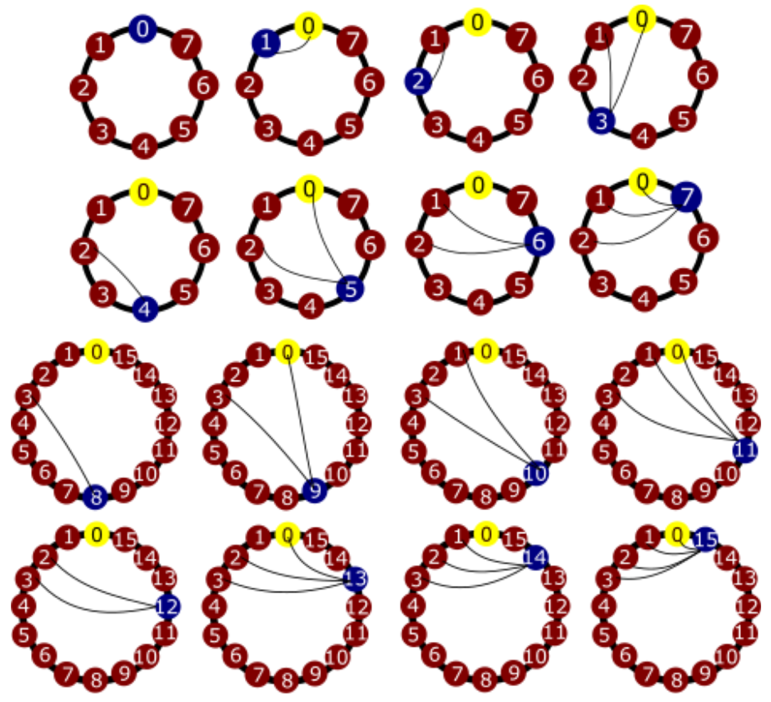
Collections of Arrows. In developing General Theory of Systems, we have to classify a system by its objects and its relations. Binary relations are collections of arrows. Every number $0\le a\le 31$ is the collection of arrows $\{x\to a\}$, for all $0\le x<a$. For example, $23=\{0\to 23,1\to 23,2\to 23,4\to 23\}$. This means we provide an isomorphism that sends $X\in \mathbb{N}$ to the set of arrows $\{x\to X\}$, for all x element of the set number X. For example, 6 is represented by the collection of arrows $\{1\to 6,2\to 6\}$ and 13 is the collection of arrows $\{0\to 13,2\to 13,3\to 13\}$ (Figure 17).

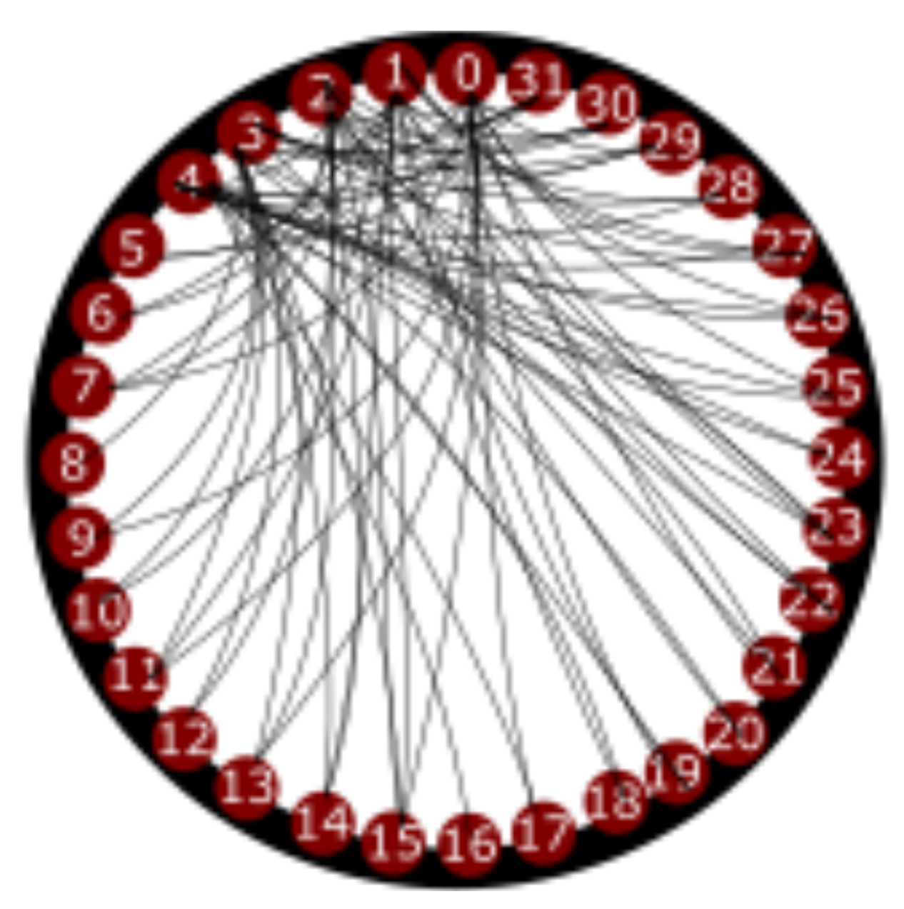
We are showing a diagram of objects and arrows to describe the structure of the natural numbers. The objects are the natural numbers $0,1,2,3\dots$, and the arrows are $0\to 1$, $0\to 3$, $0\to 5,\dots$; $1\to 2$, $1\to 3$, $1\to 6$, $1\to 7$, …; $2\to 4$, $2\to 5$, $2\to 6$, $2\to 7$, $2\to 12$, …; $3\to 8$, $3\to 9$, $3\to 10$, $3\to 11$, $3\to 12$,$\dots ;\dots$ (see Figure 18). The pattern that these relations follow is obvious $0\in {\{1+2i\}}_{i\in \mathbb{N}}$, $1\in {\{2+4i,3+4i\}}_{i\in \mathbb{N}}$, $2\in {\{4+8i,5+8i,6+8i,7+8i\}}_{i\in \mathbb{N}}$, $3\in {\{8+16i,9+16i,10+16i,11+16i,12+16i,13+16i,14+16i,15+16i\}}_{i\in \mathbb{N}}$, etc. In Figure 18, we represent the natural numbers from 0 to 31. We arrange the objects along a circumference, and start adding the arrows to obtain Figure 18:

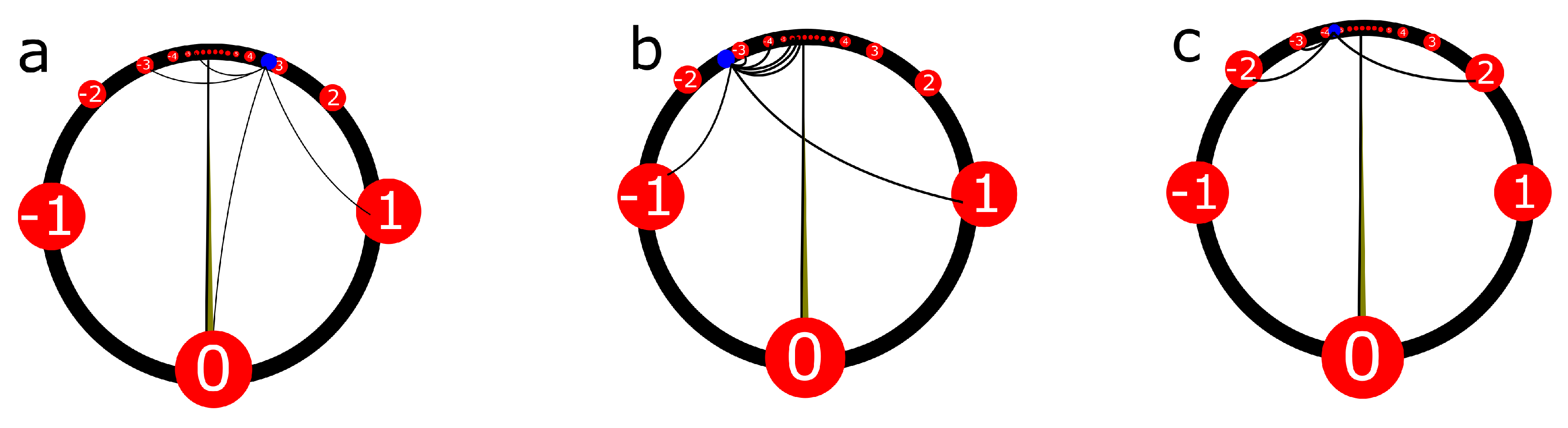
Let us transform the real number line into a circumference. The integers correspond to the discrete points (in red) of Figure 19. These have been determined by successive bisections of the circumference. Given an arbitrary point (blue) on the continuum of the circumference, we have a unique number $x\in \mathbb{R}$. At the same time, $\left|x\right|$ is a set of integers. Every real number is identified with a subset of the red points. We draw arrows from the red points, corresponding to the elements of $\left|x\right|$, into the blue point that corresponds to x.

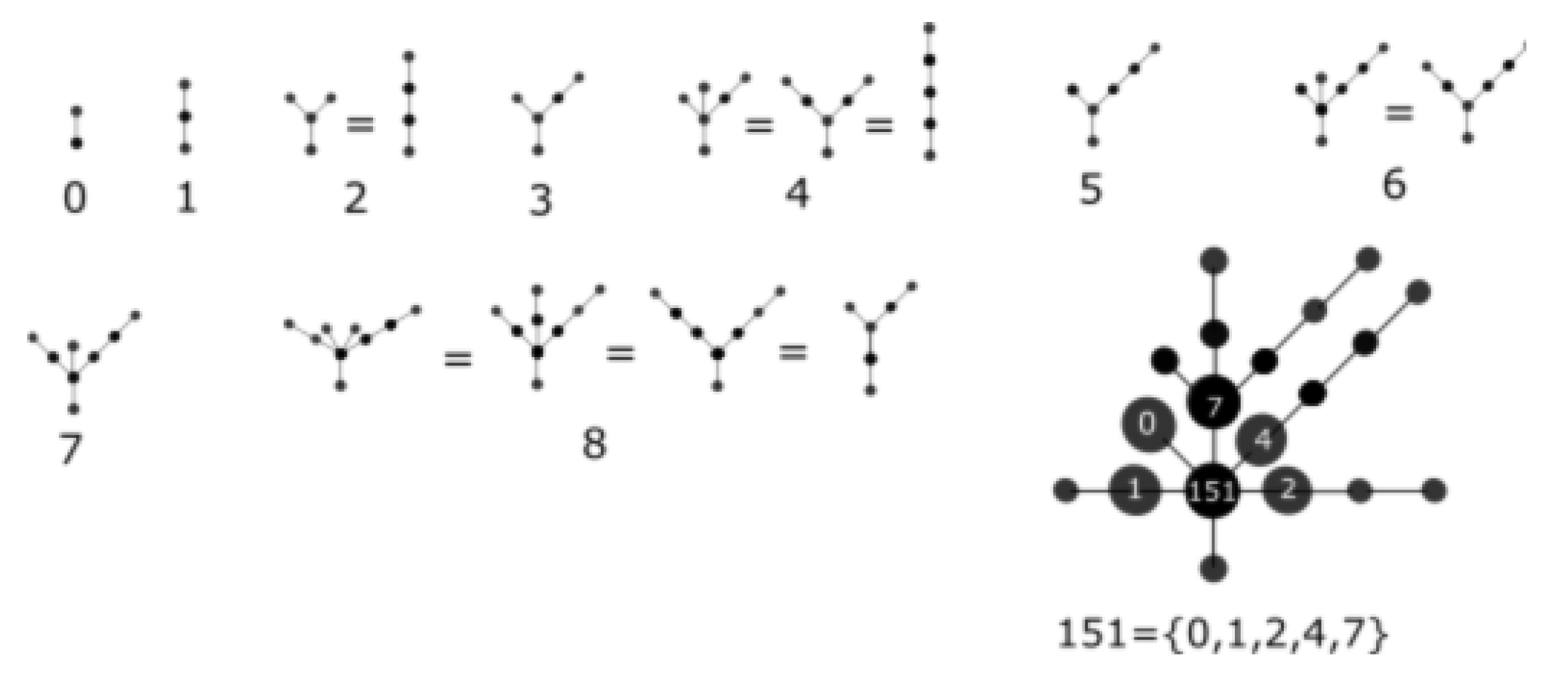
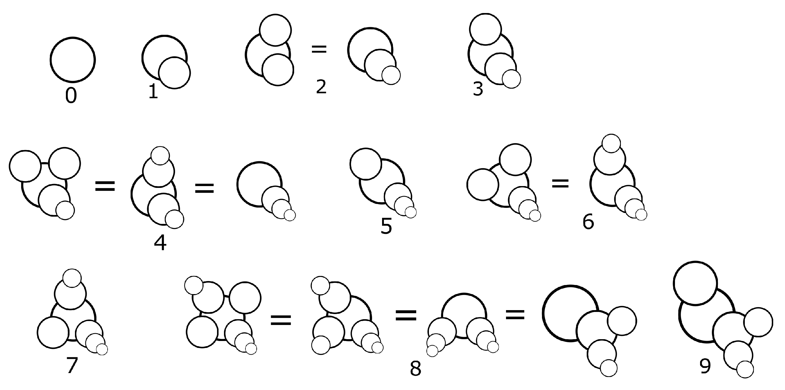
Trees. A tree is a graph of nodes and edges such that (1) We can identify a trunk: a principle edge with a finite number of branches attached to one of the nodes. All branches are attached to the same node of the trunk. (2) Each branch on the tree is a tree. (3) A single edge is a tree; we call it the 0-tree. The successor of a tree is obtained by adding a single edge to the trunk. Adding an edge to the trunk of the 0-tree gives its successor, the 1-tree, which is two edges joined together at one node. Adding an edge to the 1-tree, we find its successor, the 2-tree. If two branches are repeated on the same trunk, we substitute the two repeated branches with a single branch; the successor of these. This is called reduction. If one tree can be reduced to obtain another tree, they are in the same equivalence class. An irreducible tree is said to be in canonical form. Reducing the 2-tree, we find the canonical form (Figure 20). Adding a single edge to that, we obtain the canonical form of the 3-tree. If we add an edge to the 3-tree we have to reduce and obtain the canonical form of the 4-tree, etc. Every natural number is associated an equivalence class of trees. Every branch on the canonical tree of a set number X corresponds to a natural number $k\in X$. Every tree is made up of smaller trees, and we give a well defined method of building trees. The canonical tree corresponding to the set number X has $\#\left(X\right)$ branches. Each branch is defined in the same way.

We can represent non-negative real numbers if we define an orientation, and allow the tree to have denumerable roots. A root would be a downward branch attached to the trunk. Roots represent the negative elements of a set number.

Rings. A ring, R, is a circumference passing through the center of a denumerable number of rings $R_i$. The central circumference R is said to have degree 0. The circumferences $R_i$ are rings themselves; we say they have degree 1. Each $R_i$ is a circumference passing through the center of a denumerable set $R_i^{j_i}$ of circumferences of degree 2, and so on. A natural number n, with set number N, is represented by an equivalence class of rings. To build the canonical ring corresponding to a natural number, we draw an $R_i$, for each element of the set number $N=\{a_1,a_2,a_3,\dots \}$. That is to say, the central ring is a circumference going through $\#\left(N\right)$ circumferences; each of these a ring $R_i$. Then, $R_i$ is a circumference going through the center of $\#\left(a_i\right)$ circumferences. We apply this recursively, until we bottom out.

The equivalence relation between rings is defined similarly to trees. If we have a ring with two identical rings, we substitute these both with a single ring; the successor ring of the repeated rings. This process is called reduction. The successor ring of R is found by adding a single ring to the central circumference of R, and then finding its irreducible ring (Figure 21).

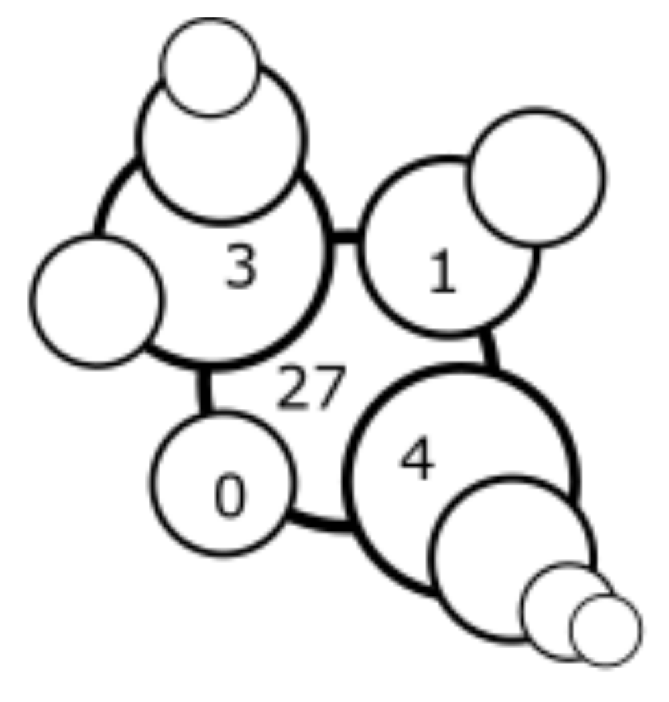
Consider the ring of the number 27 = {4, 3, 1, 0}. Then, R is a circumference passing through the center of four rings $R_1,R_2,R_3,R_4$, each representing a number of the set $\{4,3,1,0\}$ (Figure 22).

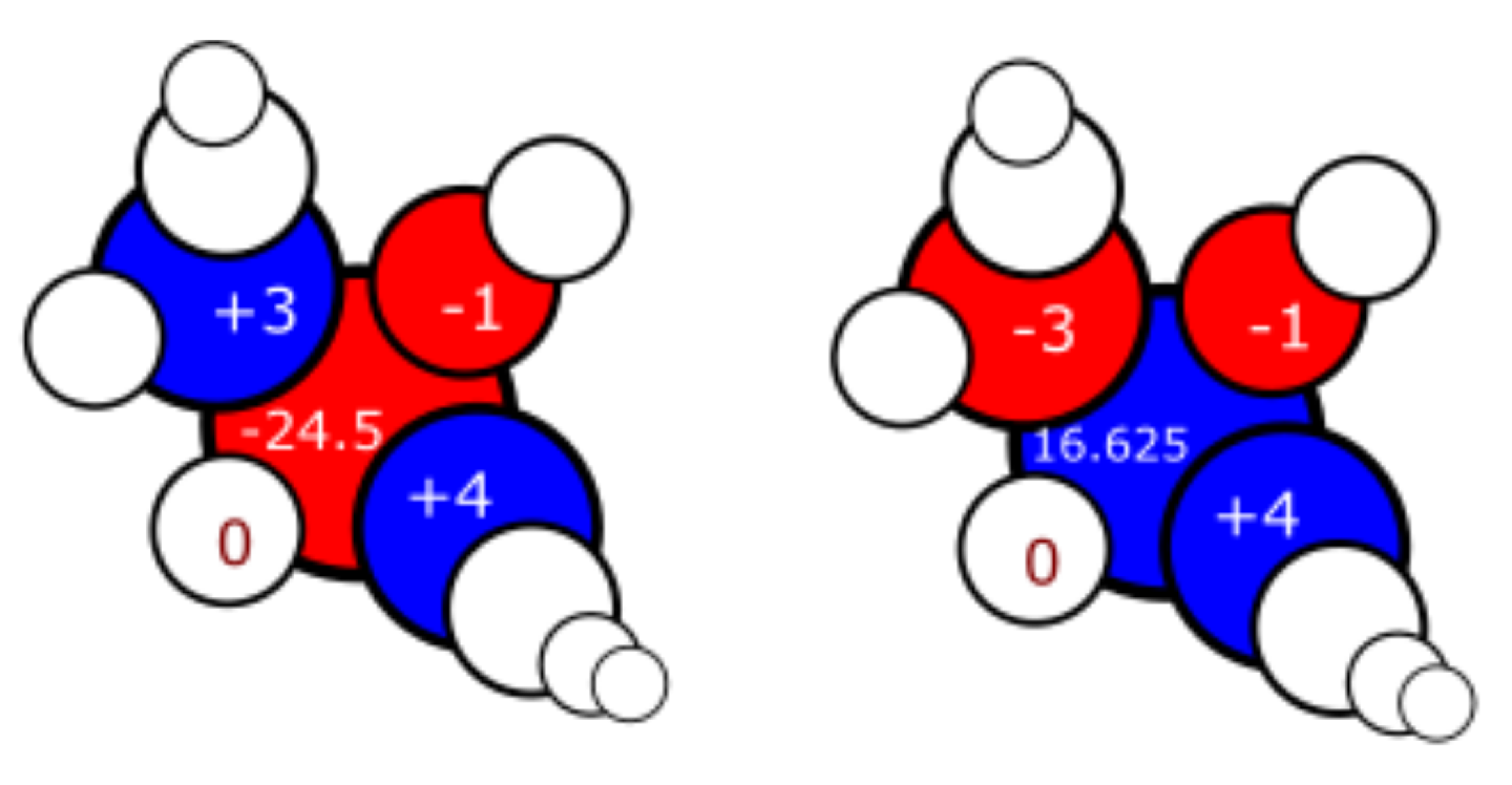
Giving a degree of freedom to the rings of degree 0 and 1, we are able to represent the set of real numbers. If the number is negative, we paint the degree 0 ring red; if it is positive, the degree 0 ring is blue. The degree 1 rings are allowed to be red or blue in order to represent negative integers; a red degree 1 ring means we have a negative power in the binary representation. A 0 ring of degree 1 is neither red nor blue because $2^0=1$ is its own reciprocal (Figure 23).

8. Conclusions

These methods and definitions are elementary, and the presentation may seem trivial and in plain sight, but constructions and proofs are not apparent. The real number system has been revisited on many occasions but has never had simple solution. The initial purpose of this investigation was to find a system theoretic treatment of numbers, as opposed to the set theoretic foundations of the classical axiomatic systems. The main goal was to propose a model of the relations of numerical systems, which reflected their true nature in the universe of sets. This work comes after an initial attempt was made in [8]. Our construction of real numbers has provided (1) New algorithms for calculating operations of real numbers; (2) Graphic representations of real numbers—we can associate numbers to certain classes of physical models. (3) We have provided a canonical set theory for arithmetic of natural numbers, and for analysis, one set being the power set of the other. We have answered Benacerraf’s identification problem [9] by giving these canonical set representations of numbers, thus proving that there is an intrinsic connection between the universe of sets and the universe of arithmetic and analysis. An extended version of these results and methods is under way. Several topics are treated in the same way. The topics include a calculus defined in terms of the order of $\mathbb{N}$. A computing device that operates using radio frequency signals emitted back and forth between two stations is tempting. Station A emits two sets of signals to station B, which then emits two signals back to station A. This process continues until the signal stabilizes (we can use this physical process to model addition, using the interpretation of energy levels). Other applications may be explored based on the graphic representations.