
Consistency of Approximation of Bernstein Polynomial-Based Direct Methods for Optimal Control
by
 , , and
Venanzio Cichella
1,*,
Isaac Kaminer
2,
Claire Walton
3,
Naira Hovakimyan
4 and
António Pascoal
5 1
Department of Mechanical Engineering, University of Iowa, Iowa City, IA 52242, USA
2
Department of Mechanical and Aerospace Engineering, Naval Postgraduate School, Monterey, CA 93940, USA
3
Department of Electrical and Computer Engineering, University of Texas at San Antonio, San Antonio, TX 78249, USA
4
Department of Mechanical Science and Engineering, University of Illinois at Urbana-Champaign, Urbana, IL 61801, USA
5
Institute for Systems and Robotics (ISR), Instituto Superior Tecnico (IST), University of Lisbon, 1049-001 Lisbon, Portugal
*
Author to whom correspondence should be addressed.
Machines 2022, 10(12), 1132; https://doi.org/10.3390/machines10121132
Submission received: 28 September 2022
/
Revised: 14 November 2022
/
Accepted: 23 November 2022
/
Published: 28 November 2022
Abstract
:Bernstein polynomial approximation of continuous function has a slower rate of convergence compared to other approximation methods. “The fact seems to have precluded any numerical application of Bernstein polynomials from having been made. Perhaps they will find application when the properties of the approximant in the large are of more importance than the closeness of the approximation.”—remarked P.J. Davis in his 1963 book, Interpolation and Approximation. This paper presents a direct approximation method for nonlinear optimal control problems with mixed input and state constraints based on Bernstein polynomial approximation. We provide a rigorous analysis showing that the proposed method yields consistent approximations of time-continuous optimal control problems and can be used for costate estimation of the optimal control problems. This result leads to the formulation of the Covector Mapping Theorem for Bernstein polynomial approximation. Finally, we explore the numerical and geometric properties of Bernstein polynomials, and illustrate the advantages of the proposed approximation method through several numerical examples.
1. Introduction
Motion planning plays an important role in enabling robotic systems to accomplish tasks assigned to them autonomously, safely and reliably. Over the past decades, many approaches to generating trajectories have been proposed. Examples include bug algorithms, artificial potential functions, roadmap path planners, cell decomposition methods, and optimal control-based trajectory generation. The reader is referred to [1,2,3,4,5,6,7,8] and references therein for detailed discussions and comparisons of these methods. Each technique has different advantages and disadvantages, and is best suited to certain types of problems. Motion planning based on optimal control, i.e., optimal motion planning, is particularly suitable for applications that require the trajectory to optimize some costs while guaranteeing satisfaction of a complex set of vehicle and problem constraints. These applications include multi-robot road search [9], coordinated tracking [10], optimal and constrained formation control [11], and adversarial swarm defense [12].
Optimal control problems that arise from robotics and motion-planning applications are, in general, very complex. Finding a closed-form solution to these problems can be difficult or even impossible, and therefore they must be solved numerically. Numerical methods include indirect and direct methods [13]. Indirect methods solve the problems by converting them into boundary value problems. Then, the solutions are found by solving systems of differential equations. On the other hand, direct methods are based on transcribing optimal control problems into nonlinear programming problems (NLPs) using a discretization scheme [6,13,14,15]. These NLPs can be solved using ready-to-use NLP solvers (e.g., MATLAB, SNOPT, etc.) and do not require calculation of costate and adjoint variables, as indirect methods do.
A wide range of direct methods that use different discretization schemes have been developed, including direct single shootings, direct multiple shooting and direct collocation methods [6,13,14,15]. The software packages that implement some of these methods (e.g., PSOPT [16], NLOptControl [17], GPOPS II [18], PROPT [19], DIDO [20] and CasADi [21]) are particularly relevant; some of these have been applied successfully to solve a wide range of real-world problems [22,23,24,25,26,27,28]. Theoretical results in the literature on direct methods include those related to consistency of approximation theory; see [29], which provides a framework to assess the convergence properties of Euler and Range–Kutta discretization schemes. Motivated by the consistency of approximation theory, direct methods that use different discretization schemes have been developed, including Pseudospectral methods based on Legendre, Chebyshev and Lagrange polynomials [28]. One drawback of direct methods is that the costate of the original optimal control problem cannot be readily obtained from the approximated solution. Nevertheless, in several applications—such as motion planning and control for safety-critical robotic systems—the knowledge of the costate is important because it allows for the evaluation of the fulfillment of necessary conditions of optimality. This evaluation, in turn, provides important insights into the validity and optimality of the solution. Therefore, approaches for obtaining estimates of the costate from direct methods have been proposed in the literature on direct collocation [30,31,32] and direct shooting [33].
In [34] we presented a direct method based on Bernstein polynomials. We showed that the geometric properties of these polynomials allow for the implementation of efficient algorithms for the computation of state and input constraints, which are particularly useful for motion planning and trajectory generation applications [35,36]. Additional works that exploit the properties of Bernstein polynomials for nonlinear optimal control can be found in [37,38,39,40,41]. Furthermore, in [42] we used the approximation properties of Bernstein polynomials to derive consistency and convergence results for the proposed direct method. In the present paper, we propose an approximation scheme for primal and dual optimal control problems based on Bernstein polynomials. In particular, we propose an approach to approximate the costate of a general non-linear optimal control problem of Bolza type using the Lagrange multipliers of the Bernstein polynomial-based discrete approximation. We derive transformations that relate the Lagrange multipliers of the nonlinear programming problem to the costate of the original optimal control problem. These transformations are often referred to as covector mapping in the literature on direct methods for optimal control [28,29,43]. Finally, we demonstrate uniform convergence properties of the method.
The paper is structured as follows: in Section 2, we present the notation and the mathematical results, which will be used later in the paper. Section 3 introduces the optimal control problem of interest and some related assumptions, and presents the approximation method based on Bernstein approximation that approximates the optimal control problem into an NLP. In Section 4 we derive the Karush–Kuhn–Tucker (KKT) conditions associated with the NLP. Section 5 compares these conditions to the first-order optimality conditions for the original optimal control problem and states the Covector Mapping Theorem for Bernstein approximation. Numerical examples are discussed in Section 6, while Section 7 highlights the significance of the theoretical findings applied to a specific multi-robot simulation scenario, namely optimal defense against swarm attacks. The paper ends with conclusions in Section 8.
2. Notation and Mathematical Background
Vector-valued functions are denoted by bold letters, , while vectors are denoted by bold letters with an upper bar, . The symbol denotes the space of functions with r continuous derivatives. denotes the space of n-vector valued functions in . denotes the Euclidean norm, .
The Bernstein basis polynomials of degree N are defined as
for , with A Nth-order Bernstein polynomial is a linear combination of Bernstein basis polynomials of order N, i.e.,
where , , are referred to as Bernstein coefficients. For the sake of generality, and with a slight abuse of terminology, in this paper, we extend the definition of a Bernstein polynomial given above to a vector of Nth-order polynomials expressed in the following form
where .
In what follows, we provide a review of numerical properties of Bernstein polynomials that are used throughout this paper. The derivative and integral of a Bernstein polynomial can be easily computed as
and
respectively.
Bernstein polynomials can be used to approximate smooth functions. Consider a n-vector valued function . The Nth order Bernstein approximation of is a vector of Bernstein polynomials computed as in (1) with and for all . Namely,
The following results hold for Bernstein approximations.
Lemma 1
(Uniform convergence of Bernstein approximation). Let on , and let be computed as in Equation (3). Then, for arbitrary order of approximation , the Bernstein approximation satisfies
where is a positive constant satisfying , and is the modulus of continuity of in [44,45,46]. Moreover, if , then
where is a positive constant satisfying and is the modulus of continuity of in [47].
Lemma 2
Lemma 3.
If on , then we have
with , where is independent of N. Moreover, if , then
The Lemma above follows directly from Lemmas 1 and 2 and Equation (2).
The following property of Bernstein polynomials is relevant to this paper.
Property 1
(End point values). The Bernstein polynomial given by Equation (1) satisfies and .
3. Problem Formulation
This paper considers the following optimal control problem:
Problem 1
(Problem P). Determine and that minimize
subject to
where and are the terminal and running costs, respectively, describes the system dynamics, is the vector of boundary conditions, and is the vector of state and input constraints.
Next, we formulate a discretized version of Problem P, here referred to as Problem , where N denotes the order of approximation. This requires that we approximate the input and state functions, the cost function, the system dynamics and the equality and inequality constraints in Problem P. First, consider the following Nth-order vectors of Bernstein polynomials:
with , , and . Let and be defined as
Let be a set of equidistant time nodes, i.e., . Then, Problem can be stated as follows:
Problem 2
(Problem ). Determine and that minimize
subject to
where , and is a small positive number that depends on N and converges uniformly to 0, i.e., .
Remark 1.
Compared to the constraints of Problem P, the dynamic and inequality constraints given by Equations (10) and (12) are relaxed. Motivated by previous work on consistency of approximation theory [29], the bound , referred to as relaxation bound, is introduced to guarantee that Problem has a feasible solution. As will become clear later, the relaxation bound can be made arbitrarily small by choosing a sufficiently large order of approximation N. Furthermore, note that when , the right-hand sides of Equations (10) and (12) are equal to zero, i.e., the difference between the constraints imposed by Problems P and vanishes.
Remark 2.
The outcome of Problem is a set of optimal Bernstein coefficients and that determine the vectors of Bernstein polynomials and , i.e.,
In our previous work, see [42], we provide theoretical results demonstrating: (i) the existence of a feasible solution to Problem , and (ii) the convergence of the pair to the optimal solution of Problem P, given by . Nevertheless, the present paper focuses on the existence and convergence of the estimates of the costates of Problem P, which are introduced next.
4. Costate Estimation for Problem P
4.1. First-Order Optimality Conditions of Problem P
We start by deriving the first-order necessary conditions for Problem P. Let be the costate trajectory, and let and be the multipliers. By defining the Lagrangian of the Hamiltonian (also known as the D-form [49]) as
where the Hamiltonian is given by
the dual of Problem P can be formulated as follows [49].
In the above problem, subscripts are used to denote partial derivatives, e.g., .
The following assumptions are imposed onto Problem .
Assumption 1.
and are continuously differentiable with respect to their arguments, and their gradients are Lipschitz continuous over the domain.
Assumption 2.
Solutions , , , and of Problem exist and satisfy , , and in .
Remark 3.
Notice that Problem implicitly assumes the absence of pure state constraints in Problem P. If the inequality constraint in Equation (7) is independent of , then the costate must also satisfy the following jump condition [49]:
where is the entry or exit time into a constrained arc in which the inequality constraint is active, and denote the left-hand side and right-hand side limits of the trajectory, respectively, and is a constant covector. For simplicity, the theoretical results that will be presented in Section 5 do not consider the jump conditions above, i.e., the inequality constraints are dependent on . Nevertheless, numerical examples will be presented in Section 6, showing the applicability of the discretization method to pure state-constrained problems.
4.2. KKT Conditions of Problem
Now, we derive the necessary conditions of Problem . Let us introduce the following Nth-order Bernstein polynomials:
with , , and , and the vector . Finally, let and be defined as
With the above notation, the Lagrangian for problem can be written as
Then, the duality of Problem can be stated as follows:
Problem 4
At this point, similarly to most results on costate estimation [50,51,52], we introduce additional conditions that must be added to Equations (10)–(12), (20) and (21) in order to obtain consistent approximations of the solutions of Problem . These conditions, often referred to as closure conditions in the literature, are given as follows:
In other words, the closure conditions are constraints that must be added to Problem so that the solution of this problem approximates the solution of Problem . We notice that the conditions given above are discrete approximations of the conditions given by Equations (16) and (17). With this setup, we define the following problem:
Problem 5
The solution of Problem presents a set of optimal Bernstein coefficients , , , (which determine the Bernstein polynomials , , and ) and a vector .
5. Feasibility and Consistency of Problem
The objective of this section is to investigate the ability of the solutions of Problem to approximate the solutions of Problem . In what follows, we first show the existence of a solution to Problem (feasibility). Second, we investigate the convergence properties of this solution as (consistency). Third, by combining these two results, we finally formulate the covector mapping theorem for Bernstein approximations, which provides a map between the solution of Problem and the solution of Problem . The main results of this section are reported in the three theorems below and summarized in Figure 1.
Theorem 1
(Feasibility). Let
where and are positive constants independent of N, and , , , , and are the moduli of continuity of , , , , and , respectively. Then Problem is feasible for arbitrary order of approximation .
Proof.
This proof follows by constructing a solution for Problem , with given by Equation (24). To this end, let , , , and be a solution of Problem , which exists by Assumption 2, and define
for all , , , with corresponding Bernstein polynomials given by
The remainder of this proof shows that , , , and given above satisfy Equations (20)–(23). The satisfaction of Equations (10)–(12) can be demonstrated using a proof similar to the one of [42], and is thus omitted. We start by defining the Bernstein coefficients and as follows
with corresponding Bernstein polynomials given by
Notice that
Combining Equations (26), (27) and (29) and using Assumption 2 and Lemma 1, we get
where and , and are the moduli of continuity of , and , respectively.
Now, we show that the bound in Equation (20) is satisfied. Using Equation (30), and adding and subtracting , we get
Using Equation (14), the above inequality reduces to
where we used the bounds in Equation (31) together with the Lipschitz assumption on (see Assumptions 1). Finally, from using Assumptions 1 and 2, it follows that and are bounded on with bounds and , respectively. Therefore, we get
which implies that the bound in Equation (20) is satisfied with given by Equation (24) and . Similarly,
which proves that Equation (20) holds.
Now, consider the left equation in (21). For , we have
Substituting and , the equation above can be written as
Notice that the following inequalities are satisfied:
for some positive , , and independent of N. Proof of the above inequalities is given in Appendix A. Then, the combination of Equations (33) and (34) yields the following inequality
with . Using integration by parts, we have . Thus, since , the above inequality becomes
Finally, using Equations (15) and (16), the above inequality reduces to the left condition in Equation (21) for , with given by Equation (24) and . The same condition for can be shown to be satisfied using an identical argument. The stationarity condition in the right of Equation (21) can also be verified similarly, and the computations are thus omitted. To show that the closure condition (22) is satisfied, we use the definitions in Equations (26) and (27) together with the end point values property of Bernstein polynomials, Property 1 in Section 2, which gives
where the last equality follows from Equation (16). An identical argument can be used to show that the closure condition (23) holds, thus completing the proof of Theorem 1.
Corollary 1.
If solutions , , , and of Problem exist and satisfy , , , and in , then Theorem 1 holds with and where and are positive constants independent of the order of approximation, N.
□
Proof.
The proof of Corollary 1 follows easily by applying Lemma 2 to the proof of Theorem 1.
Remark 4.
We notice that for arbitrarily small scalar , there exists such that for all , we have ; i.e., the relaxation bound in Problem can be made arbitrarily small by choosing sufficiently large N.
Theorem 2 (Consistency)
Let be a sequence of solutions of Problem . Consider the sequence of transformed solutions , with
and the corresponding polynomial approximation . Assume that the latter has a uniform accumulation point, i.e.,
and assume , , and are continuous on . Then,
is a solution of Problem .
□
Proof.
The objective is to show that and satisfy Equations (5)–(6) and (14)–(18). The satisfaction of Equations (5)–(7) has been demonstrated in ([42] [Proof of Theorem 2]). We start by showing Equation (14), and we do so using a proof by contradiction. Assume that do not satisfy Equation (14). Then, there exists , such that
Since the nodes are dense in , there exists a sequence of indices , such that
which implies
Theorem 3
(Covector Mapping Theorem). Under the same assumptions of Theorems 1 and 2, when , the covector mapping
is a bijective mapping between the solution of Problem and the solution of Problem .
Proof.
The above result follows directly from Theorems 1 and 2. In fact, if
is a solution to Problem , which exists by Assumption 2, then from Theorem 1, it follows that is a solution to Problem (see Equations (26)–(28)). Conversely, by using Equation (37), a solution
that solves Problem provides a solution
that converges to a solution to Problem (see Theorem 2). □
Remark 5.
Define the Hamiltonian approximation
then, Theorem 3 implies
6. Numerical Examples
6.1. Example 1: 1D Minimum Time Problem
The first example we consider is the classical minimum time problem for a double integrator plant.
subject to
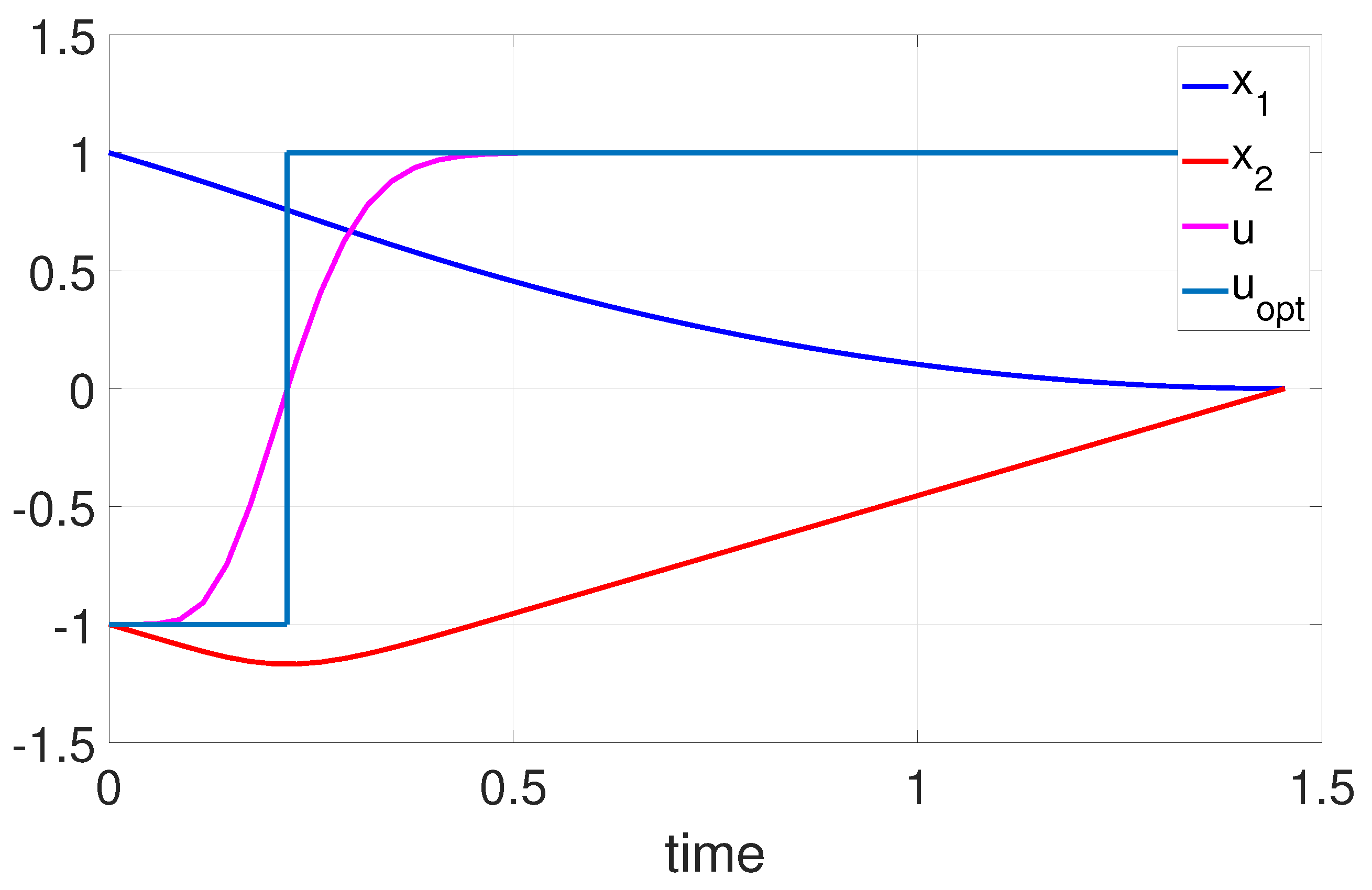
The analytical solution to this problem is well known: the optimal control input is bang-bang and the Hamiltonian along the optimal trajectories is equal to −1 [53]. Figure 2 includes plots of the state and control trajectories for this problem for , as well as a graph of the analytical solution. It is clear that the Bernstein polynomial solution captures the switching time precisely and closely approximates the optimal control input solution. Figure 3 includes the plot of the Hamiltonian approximation computed using Covector Mapping Theorem. As expected, it is equal to −1 with the exception of a small bump around the switching time.
6.2. Example 2: 3D Minimum Time Problem
In this example, we consider a minimum-time problem for a simplified 3D model of a multi-rotor drone. The vehicle is asked to reach the origin in minimum time from a given initial condition with all the control inputs bounded by . Unlike Example 1, there is no known analytical solution to this problem. However, we know that the Hamiltonian along the optimal trajectories is equal to −1 [53].
subject to
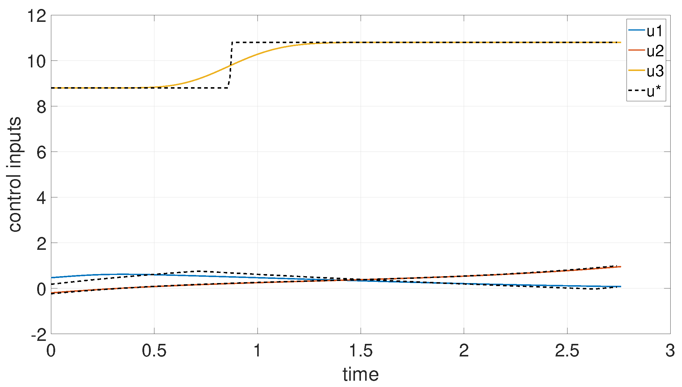
Figure 4 shows the 3D plot of the position of the vehicle. The vehicle clearly reaches the origin from the given initial condition. Figure 5 includes graphs of the control inputs. They satisfy the bound imposed in the problem formulation. Finally, Figure 6 shows the plot of the Hamiltonian approximation . It is equal to −1, as predicted by theory, thus indicating that the solution obtained is indeed close to optimal.
7. Defense against a Swarm Attack
The numerical analysis presented here involves a scenario in which an enemy swarm is attempting to destroy an high-value unit (HVU). The HVU is defended by a number of defending agents whose trajectories are optimized to maximize the probability of the HVU survival. The attacking agents dynamics are defined using Leonard swarm dynamics model [54]. A virtual leader is guiding the attacking swarm towards the HVU’s position. The attacking and defending agents are equipped with weapons systems which allow them to inflict damage on each other. The attacking agents inflict damage on the defending agents and try to destroy the HVU. The defending agents inflict damage on the attacking agents and attempt to destroy them or herd them away.
Attacking agent has position and defending agent has position . The equations of motion for attacker i is
for . There are four terms in this equation, representing: (1) attractive and repulsive forces from other attacking agents j, where is the distance between attackers i and j; (2) a constant “virtual leader” force with magnitude K pulling them toward the HVU’s position, where and h is the position of the HVU; (3) purely repulsive forces due to defending agents, where is the distance between attacker i and defender k; and (4) a damping force proportional to the .
For the mathematical forms of and , we have chosen the Leonard model [54], i.e., and can be written as gradients of a scalar potential functions that depends only on and . The force is repulsive when , attractive when and zero when . For , we only keep the repulsive term (since attackers should not be attracted to defenders), i.e., is repulsive when and zero when .
Defending agent i’s dynamics are given by
where the absolute value of each element of , is bounded by .
Mutual attrition model: for hostile swarm engagements, agents are equipped with some weapons systems. The likelihood of destruction of an agent depends on its position (how close it has come to enemies) as well as the positions of those enemy agents, since each agent’s ability to inflict damage is contingent on its own survival. To model this mutual attrition, we use a damage function to track the probability that defender k is destroyed by a shot from attacker i, and vice versa. We choose a cumulative normal distribution function, , to model the damage function [55]. Next, we define (i) the attrition rate at which attacker i is destroyed due to defender k, , (ii) the attrition rate of defender k due to attacker i, , and (iii) the attrition rate of the HVU, , as follows:
In the above equation is a defender Poisson parameter that corresponds to the range of the defenders’ weapons, is a defender Poisson parameter that corresponds to the defenders’ rate of fire, is an attacker Poisson parameter that corresponds to the attackers’ range and is an attacker Poisson parameter that corresponds to the attackers’ rate of fire. The probability of defender k destroying attacker i during a time interval of duration is weighted by the current survival probability of defender k, . Thus, the probability that defender k will destroy attacker i during a given time interval is . Assuming independence (i.e., defenders do not coordinate their fire), the expression represents the probability that ith attacker would survive during a time interval due to attrition from all defenders. Therefore, the survival probability of attacker i is governed by
where we assumed that probabilities of attacker i survival , are independent for any . Similarly, the survival probability of defender k and the survival probability of the HVU are governed by
Initial conditions are set to for all agents and the HVU.
The optimal control problem at hand can be expressed as Problem P by properly rescaling the time variable, i.e., ; see Equations (4)–(7). In particular, we seek to maximize the probability of HVU survival at the terminal time (), i.e., minimize The system’s state includes the attacker and the defender positions and velocities, as well as probabilities of the attacker and defender survivals and the probability of the HVU survival:
where is the velocity of the i-th attacker and is the velocity of the k-th defender. The control input vector is defined by stacking accelerations of each defender . Using definitions of the system’s state and control inputs the system dynamics function is given by concatenation of Equations (40), (41), (45), and (46). Finally, the function in our case becomes a function of defender control inputs only and includes .
Figure 7 shows results for an optimization with one defender protecting an HVU against a swarm of five attackers for . The HVU is at the origin and the defender trajectory is color purple. The defender has a 50% larger weapons range (), as well as double the fire rate with respect to the attackers (). The defender initially herds the attackers on his right away from HVU than approaches the HVU and similarly herds the attackers to his left away from the HVU. Figure 8 illustrates the control inputs that drive the motion of the defender. Unlike minimum time problems, e.g., the previous example, in this case, the inequality constraints on the control input are never active. Figure 9 shows a sequence of the Hamiltonian approximations . The sequence clearly converges to zero, indicating that the final numerical solution for is indeed a close approximation of the true optimal solution.
8. Conclusions
This paper proposed a numerical method for costate estimation of nonlinear constrained optimal control problems using Bernstein polynomials. A rigorous analysis is provided that shows convergence of the costate estimates to the dual variables of the continuous-time problem. To this end, a set of conditions are derived under which the Karush–Kuhn–Tucker multipliers of the NLP converge to the costates of the optimal control problem. This led to the formulation of the Covector Mapping Theorem for Bernstein approximation. The theoretical findings are validated through several numerical examples.
Author Contributions
Conceptualization, V.C., I.K., A.P., C.W.; methodology, V.C., I.K., A.P., C.W.; software, V.C, I.K.; validation, V.C, I.K., C.W.; investigation, V.C., I.K., A.P., C.W.; resources, V.C., I.K., A.P., N.H.; writing—original draft preparation, V.C., I.K.; writing—review and editing, V.C, I.K.; supervision, V.C., I.K., A.P., C.W., N.H.; project administration, V.C.; funding acquisition, V.C., I.K., A.P., N.H. All authors have read and agreed to the published version of the manuscript.
Funding
Venanzio Cichella was supported by Amazon, by the Office of Naval Research (grants N000141912106 and N000142112091), and by the National Science Foundation (grant 2136298). Antonio Pascoal was supported by H2020-EU.1.2.2—FET Proactive RAMONES (grant GA 101017808) and LARSyS-FCT (grant UIDB/50009/2020). Isaac Kaminer was supported by the Office of Naval Research (grants N0001421WX01974, N0001419WX00155, N0001422WX01906) and NPS CRUSER. Naira Hovakimyan was supported by NASA ULI (grant #80NSSC22M0070) and NSF RI (grant 2133656).
Institutional Review Board Statement
Not applicable.
Informed Consent Statement
Not applicable.
Data Availability Statement
Not applicable.
Conflicts of Interest
The authors declare no conflict of interest.
Appendix A. Proof of Equation (34)
Let us focus on Equation (34a). Adding and subtracting , we have
Using Lemma 3 and continuity of and , the first term on the right-hand side of the inequality above satisfies
where is used to denote the modulus of continuity of the product
with being a bounded function due to its continuity over a bounded domain. Denote its bound as . Notice that is bounded, as . Then, using the properties of the modulus of continuity, we get
where is the modulus of continuity of , and is a positive constant independent of N. Furthermore, we have
where is the Lipschitz constant of , , , and and are the moduli of continuity of and , respectively. Combining Equations (A2) and (A3) with Equation (A1) yields
which proves the bound in Equation (34a). The bounds in Equation (34b–d) follow easily using an identical argument.
References
- Ng, J.; Bräunl, T. Performance comparison of bug navigation algorithms. J. Intell. Robot. Syst. 2007, 50, 73–84. [Google Scholar] [CrossRef]
- Khatib, O. Real-time obstacle avoidance for manipulators and mobile robots. In Autonomous Robot Vehicles; Springer: Berlin/ Heidelberg, Germany, 1986; pp. 396–404. [Google Scholar]
- Siegwart, R.; Nourbakhsh, I.R.; Scaramuzza, D. Introduction to Autonomous Mobile Robots; MIT Press: Cambridge, MA, USA, 2011. [Google Scholar]
- Choset, H.M. Principles of Robot Motion: Theory, Algorithms, and Implementation; MIT Press: Cambridge, MA, USA, 2005. [Google Scholar]
- Latombe, J.C. Robot Motion Planning; Springer Science & Business Media: Berlin/Heidelberg, Germany, 2012; Volume 124. [Google Scholar]
- Betts, J.T. Survey of numerical methods for trajectory optimization. J. Guid. Control Dyn. 1998, 21, 193–207. [Google Scholar] [CrossRef] [Green Version]
- Von Stryk, O.; Bulirsch, R. Direct and indirect methods for trajectory optimization. Ann. Oper. Res. 1992, 37, 357–373. [Google Scholar] [CrossRef]
- LaValle, S.M. Planning Algorithms; Cambridge University Press: Cambridge, UK, 2006. [Google Scholar]
- Cichella, V. Cooperative Autonomous Systems: Motion Planning and Coordinated Tracking Control for Multi-Vehicle Missions. Ph.D. Thesis, University of Illinois at Urbana-Champaign, Champaign, IL, USA, 2018. [Google Scholar]
- Cichella, V.; Kaminer, I.; Dobrokhodov, V.; Xargay, E.; Choe, R.; Hovakimyan, N.; Aguiar, A.P.; Pascoal, A.M. Cooperative Path-Following of Multiple Multirotors over Time-Varying Networks. IEEE Trans. Autom. Sci. Eng. 2015, 12, 945–957. [Google Scholar] [CrossRef]
- Sun, X.; Cassandras, C.G. Optimal dynamic formation control of multi-agent systems in constrained environments. Automatica 2016, 73, 169–179. [Google Scholar] [CrossRef] [Green Version]
- Walton, C.; Kaminer, I.; Gong, Q.; Clark, A.H.; Tsatsanifos, T. Defense against adversarial swarms with parameter uncertainty. Sensors 2022, 22, 4773. [Google Scholar] [CrossRef]
- Rao, A.V. A survey of numerical methods for optimal control. Adv. Astronaut. Sci. 2009, 135, 497–528. [Google Scholar]
- Betts, J.T. Practical Methods for Optimal Control and Estimation Using Nonlinear Programming; SIAM: Philadelphia, PA, USA, 2010. [Google Scholar]
- Conway, B.A. A survey of methods available for the numerical optimization of continuous dynamic systems. J. Optim. Theory Appl. 2012, 152, 271–306. [Google Scholar] [CrossRef]
- Becerra, V.M. Solving complex optimal control problems at no cost with PSOPT. In Proceedings of the 2010 IEEE International Symposium on Computer-Aided Control System Design, Yokohama, Japan, 8–10 September 2010; pp. 1391–1396. [Google Scholar]
- Febbo, H.; Jayakumar, P.; Stein, J.L.; Ersal, T. NLOptControl: A modeling language for solving optimal control problems. arXiv 2020, arXiv:2003.00142. [Google Scholar]
- Patterson, M.A.; Rao, A.V. GPOPS-II: A MATLAB software for solving multiple-phase optimal control problems using hp-adaptive Gaussian quadrature collocation methods and sparse nonlinear programming. ACM Trans. Math. Softw. (TOMS) 2014, 41, 1–37. [Google Scholar] [CrossRef] [Green Version]
- Rutquist, P.E.; Edvall, M.M. Propt—Matlab Optimal Control Software; Tomlab Optimization Inc.: Washington, DC, USA, 2010. [Google Scholar]
- Ross, I.M. Enhancements to the DIDO Optimal Control Toolbox. arXiv 2020, arXiv:2004.13112. [Google Scholar]
- Andersson, J.A.; Gillis, J.; Horn, G.; Rawlings, J.B.; Diehl, M. CasADi: A software framework for nonlinear optimization and optimal control. Math. Program. Comput. 2019, 11, 1–36. [Google Scholar] [CrossRef]
- Fahroo, F.; Ross, I.M. On discrete-time optimality conditions for pseudospectral methods. In Proceedings of the AIAA/AAS Astrodynamics Specialist Conference and Exhibit, Keystone, CO, USA, 21–24 August 2006; p. 6304. [Google Scholar]
- Bollino, K.; Lewis, L.R.; Sekhavat, P.; Ross, I.M. Pseudospectral optimal control: A clear road for autonomous intelligent path planning. In Proceedings of the AIAA Infotech@ Aerospace 2007 Conference and Exhibit, Rohnert Park, CA, USA, 7–10 May 2007; p. 2831. [Google Scholar]
- Gong, Q.; Lewis, R.; Ross, M. Pseudospectral motion planning for autonomous vehicles. J. Guid. Control. Dyn. 2009, 32, 1039–1045. [Google Scholar] [CrossRef]
- Bedrossian, N.S.; Bhatt, S.; Kang, W.; Ross, I.M. Zero-propellant maneuver guidance. IEEE Control. Syst. 2009, 29. [Google Scholar]
- Bollino, K.; Lewis, L.R. Collision-free multi-UAV optimal path planning and cooperative control for tactical applications. In Proceedings of the AIAA Guidance, Navigation and Control Conference and Exhibit, Honolulu, HI, USA, 18–21 August 2008; p. 7134. [Google Scholar]
- Bedrossian, N.; Bhatt, S.; Lammers, M.; Nguyen, L.; Zhang, Y. First Ever Flight Demonstration of Zero Propellant Maneuver (TM) Attitute Control Concept. In Proceedings of the AIAA Guidance, Navigation and Control Conference and Exhibit, Hilton Head, SC, USA, 20–23 August 2007; p. 76734. [Google Scholar]
- Ross, I.M.; Karpenko, M. A review of pseudospectral optimal control: From theory to flight. Annu. Rev. Control. 2012, 36, 182–197. [Google Scholar] [CrossRef]
- Polak, E. Optimization: Algorithms and Consistent Approximations; Springer: Berilin, Germany, 1997. [Google Scholar]
- Fahroo, F.; Ross, I.M. Costate estimation by a Legendre pseudospectral method. J. Guid. Control Dyn. 2001, 24, 270–277. [Google Scholar] [CrossRef]
- Darby, C.L.; Garg, D.; Rao, A.V. Costate estimation using multiple-interval pseudospectral methods. J. Spacecr. Rocket. 2011, 48, 856–866. [Google Scholar] [CrossRef]
- Hager, W.W. Runge-Kutta methods in optimal control and the transformed adjoint system. Numer. Math. 2000, 87, 247–282. [Google Scholar] [CrossRef]
- Grimm, W.; Markl, A. Adjoint estimation from a direct multiple shooting method. J. Optim. Theory Appl. 1997, 92, 263–283. [Google Scholar] [CrossRef]
- Cichella, V.; Kaminer, I.; Walton, C.; Hovakimyan, N. Optimal Motion Planning for Differentially Flat Systems Using Bernstein Approximation. IEEE Control Syst. Lett. 2018, 2, 181–186. [Google Scholar] [CrossRef]
- Kielas-Jensen, C.; Cichella, V. BeBOT: Bernstein polynomial toolkit for trajectory generation. In Proceedings of the 2019 IEEE/RSJ International Conference on Intelligent Robots and Systems (IROS), Venetian Macao, Macau, 3–8 November 2019; pp. 3288–3293. [Google Scholar]
- Kielas-Jensen, C.; Cichella, V.; Berry, T.; Kaminer, I.; Walton, C.; Pascoal, A. Bernstein Polynomial-Based Method for Solving Optimal Trajectory Generation Problems. Sensors 2022, 22, 1869. [Google Scholar] [CrossRef] [PubMed]
- Ricciardi, L.A.; Vasile, M. Direct transcription of optimal control problems with finite elements on Bernstein basis. J. Guid. Control Dyn. 2018. [Google Scholar] [CrossRef]
- Choe, R.; Puig-Navarro, J.; Cichella, V.; Xargay, E.; Hovakimyan, N. Cooperative Trajectory Generation Using Pythagorean Hodograph Bézier Curves. J. Guid. Control Dyn. 2016, 39, 1744–1763. [Google Scholar] [CrossRef]
- Ghomanjani, F.; Farahi, M.H. Optimal control of switched systems based on Bezier control points. Int. J. Intell. Syst. Appl. 2012, 4, 16. [Google Scholar] [CrossRef]
- Huo, M.; Yang, L.; Peng, N.; Zhao, C.; Feng, W.; Yu, Z.; Qi, N. Fast costate estimation for indirect trajectory optimization using Bezier-curve-based shaping approach. Aerosp. Sci. Technol. 2022, 126, 107582. [Google Scholar] [CrossRef]
- Zhao, Z.; Kumar, M. Split-bernstein approach to chance-constrained optimal control. J. Guid. Control Dyn. 2017, 40, 2782–2795. [Google Scholar] [CrossRef]
- Cichella, V.; Kaminer, I.; Walton, C.; Hovakimyan, N.; Pascoal, A.M. Optimal Multi-Vehicle Motion Planning using Bernstein Approximants. IEEE Trans. Autom. Control 2020. [Google Scholar] [CrossRef]
- Schwartz, A.; Polak, E. Consistent approximations for optimal control problems based on Runge–Kutta integration. SIAM J. Control Optim. 1996, 34, 1235–1269. [Google Scholar] [CrossRef]
- Bojanic, R.; Cheng, F. Rate of convergence of Bernstein polynomials for functions with derivatives of bounded variation. J. Math. Anal. Appl. 1989, 141, 136–151. [Google Scholar] [CrossRef]
- Popoviciu, T. Sur l’approximation des fonctions convexes d’ordre supérieur. Mathematica 1935, 10, 49–54. [Google Scholar]
- Sikkema, P. Der wert einiger konstanten in der theorie der approximation mit Bernstein-Polynomen. Numer. Math. 1961, 3, 107–116. [Google Scholar] [CrossRef]
- Powell, M.J.D. Approximation Theory and Methods; Cambridge University Press: Cambridge, UK, 1981. [Google Scholar]
- Floater, M.S. On the convergence of derivatives of Bernstein approximation. J. Approx. Theory 2005, 134, 130–135. [Google Scholar] [CrossRef]
- Hartl, R.F.; Sethi, S.P.; Vickson, R.G. A survey of the maximum principles for optimal control problems with state constraints. SIAM Rev. 1995, 37, 181–218. [Google Scholar] [CrossRef]
- Garg, D.; Patterson, M.A.; Francolin, C.; Darby, C.L.; Huntington, G.T.; Hager, W.W.; Rao, A.V. Direct trajectory optimization and costate estimation of finite-horizon and infinite-horizon optimal control problems using a Radau pseudospectral method. Comput. Optim. Appl. 2011, 49, 335–358. [Google Scholar] [CrossRef] [Green Version]
- Gong, Q.; Ross, I.M.; Kang, W.; Fahroo, F. Connections between the covector mapping theorem and convergence of pseudospectral methods for optimal control. Comput. Optim. Appl. 2008, 41, 307–335. [Google Scholar] [CrossRef]
- Singh, B.; Bhattacharya, R.; Vadali, S.R. Verification of optimality and costate estimation using Hilbert space projection. J. Guid. Control Dyn. 2009, 32, 1345–1355. [Google Scholar] [CrossRef]
- Kirk. Optimal Control Theory: An Introduction; Prentice-Hall: Hoboken, NJ, USA, 1970. [Google Scholar]
- Ogren, P.; Fiorelli, E.; Leonard, N.E. Cooperative control of mobile sensor networks: Adaptive gradient climbing in a distributed environment. IEEE Trans. Autom. Control 2004, 49, 1292–1302. [Google Scholar] [CrossRef] [Green Version]
- Washburn, A.; Kress, M. Combat Modeling; Springer: Berlin/Heidelberg, Germany, 2009. [Google Scholar]
- Walton, C.; Lambrianides, P.; Kaminer, I.; Royset, J.; Gong, Q. Optimal motion planning in rapid-fire combat situations with attacker uncertainty. Naval Res. Logist. 2018, 65, 101–119. [Google Scholar] [CrossRef]
- Cichella, V.; Kaminer, I.; Walton, C.; Hovakimyan, N.; Pascoal, A. Bernstein approximation of optimal control problems. arXiv 2018, arXiv:1812.06132. [Google Scholar]
- Cichella, V.; Kaminer, I.; Walton, C.; Hovakimyan, N.; Pascoal, A.M. Consistent approximation of optimal control problems using Bernstein polynomials. In Proceedings of the 2019 IEEE 58th Conference on Decision and Control (CDC), Nice, France, 11–13 December 2019; pp. 4292–4297. [Google Scholar]
Figure 1.
Diagram of the covector mapping principle for Bernstein approximation. The solution to Problem converges to that of Problem as .
Figure 1.
Diagram of the covector mapping principle for Bernstein approximation. The solution to Problem converges to that of Problem as .

Figure 2.
Example 1: state trajectories and , and control input . The control input approximates the optimal solution (bang-bang).
Figure 2.
Example 1: state trajectories and , and control input . The control input approximates the optimal solution (bang-bang).

Figure 3.
Example 1: the approximated Hamiltonian converges to the Hamiltonian of the problem, i.e., . See Theorem 3 and Remark 5.
Figure 3.
Example 1: the approximated Hamiltonian converges to the Hamiltonian of the problem, i.e., . See Theorem 3 and Remark 5.

Figure 4.
Example 2: 3D position plot, i.e., . The solid line represents the solution obtained with , while the dashed line depicts the (near optimal) solution obtained with .
Figure 4.
Example 2: 3D position plot, i.e., . The solid line represents the solution obtained with , while the dashed line depicts the (near optimal) solution obtained with .

Figure 5.
Example 2: Control inputs, i.e., vehicle’s acceleration along the three axis. The solid lines represent the solution obtained with , while the dashed lines depict the (near optimal) solution obtained with .
Figure 5.
Example 2: Control inputs, i.e., vehicle’s acceleration along the three axis. The solid lines represent the solution obtained with , while the dashed lines depict the (near optimal) solution obtained with .

Figure 6.
Example 2: the approximated Hamiltonian converges to the Hamiltonian of the problem, i.e., . See Theorem 3 and Remark 5.
Figure 6.
Example 2: the approximated Hamiltonian converges to the Hamiltonian of the problem, i.e., . See Theorem 3 and Remark 5.

Figure 7.
Defense against swarm attack. The plot shows optimal trajectory of one defender (purple) protecting a high-value unit (positioned at the origin) against five attackers.
Figure 7.
Defense against swarm attack. The plot shows optimal trajectory of one defender (purple) protecting a high-value unit (positioned at the origin) against five attackers.

Figure 8.
Defense against swarm attack. The plot shows the time history of the control input.

Figure 9.
Hamiltonian Convergence. The plot shows a sequence of the Hamiltonian approximations , indicating that the numerical solution converges to the true optimal solution.
Figure 9.
Hamiltonian Convergence. The plot shows a sequence of the Hamiltonian approximations , indicating that the numerical solution converges to the true optimal solution.

Publisher’s Note: MDPI stays neutral with regard to jurisdictional claims in published maps and institutional affiliations. |
© 2022 by the authors. Licensee MDPI, Basel, Switzerland. This article is an open access article distributed under the terms and conditions of the Creative Commons Attribution (CC BY) license (https://creativecommons.org/licenses/by/4.0/).
Share and Cite
MDPI and ACS Style
Cichella, V.; Kaminer, I.; Walton, C.; Hovakimyan, N.; Pascoal, A. Consistency of Approximation of Bernstein Polynomial-Based Direct Methods for Optimal Control. Machines 2022, 10, 1132. https://doi.org/10.3390/machines10121132
AMA Style
Cichella V, Kaminer I, Walton C, Hovakimyan N, Pascoal A. Consistency of Approximation of Bernstein Polynomial-Based Direct Methods for Optimal Control. Machines. 2022; 10(12):1132. https://doi.org/10.3390/machines10121132
Chicago/Turabian StyleCichella, Venanzio, Isaac Kaminer, Claire Walton, Naira Hovakimyan, and António Pascoal. 2022. "Consistency of Approximation of Bernstein Polynomial-Based Direct Methods for Optimal Control" Machines 10, no. 12: 1132. https://doi.org/10.3390/machines10121132
Note that from the first issue of 2016, this journal uses article numbers instead of page numbers. See further details here.