Optimization of EDM Machinability of Hastelloy C22 Super Alloys

Abstract

In this study, machinability tests were carried out on a corrosion-resistant superalloy subjected to shallow (SCT) and deep cryogenic treatment (DCT) via electrical discharge machining (EDM), and the effect of the cryogenic treatment types applied to the material on the EDM processing performance was investigated. Experimental parameters, including pulse-on time (300, 400 and 500 μs), peak current (A) (6 and 10 A) and material types (untreated and treated with SCT and DCT), were used to construct the full factorial experimental design. The resulting average surface roughness (Ra) and material removal rate (MRR) results were optimized using the Taguchi L₁₈ method. According to the Taguchi-based gray relational analysis, the optimal parameters for both Ra and MRR were determined as cryogenic treatment, pulse-on time and peak current, respectively. The response table obtained using the Taguchi method showed the most effective factors as A₁B_lC₃ for Ra and A₂B₂C₁ for MRR values. According to the ANOVA results for determining parameters affecting performance, peak current was the most effective factor for average surface roughness and MRR, at 74.79% and 86.43%, respectively. When examined in terms of Taguchi-gray relational degrees, the optimal parameters for both Ra and MRR were observed in the experiment performed with the SCT sample at a peak current of 6 A and 300 μs pulse-on time.

1. Introduction

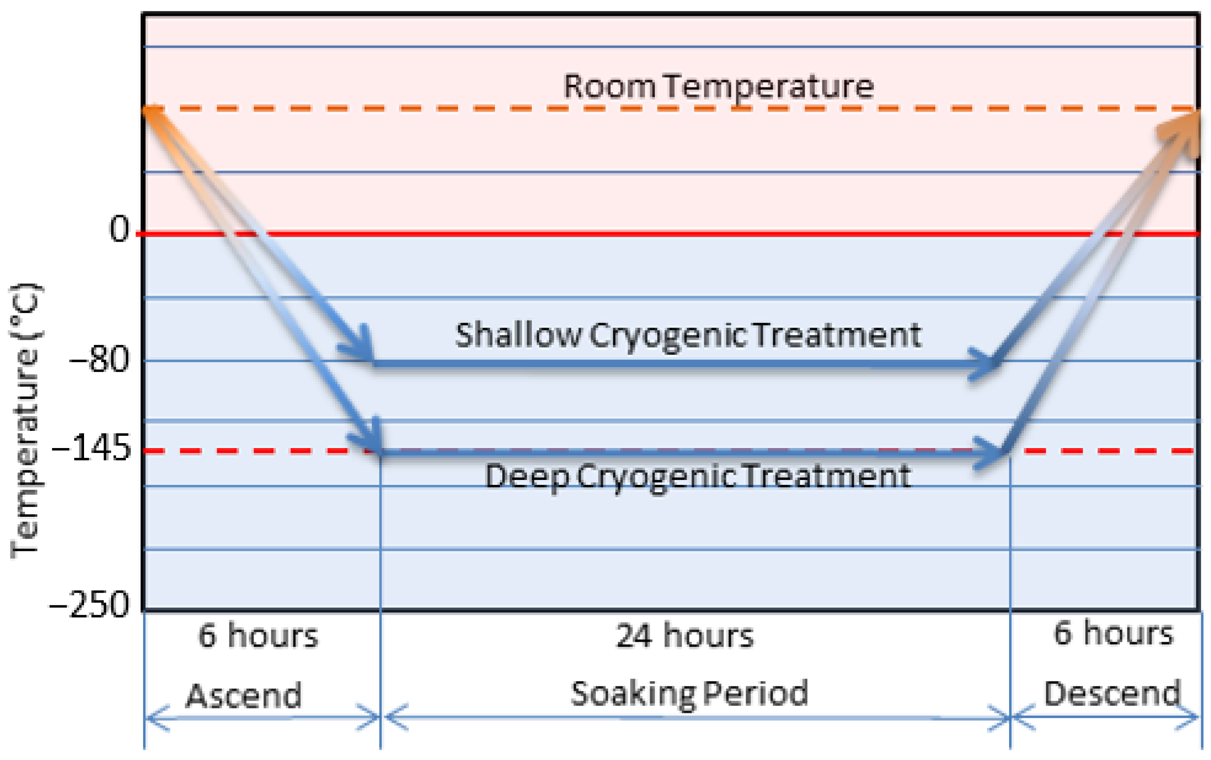
Cryogenic treatment is a type of heat treatment applied at low temperatures that is used to improve the mechanical and physical properties of materials. Cryogenic treatment is applied to a wide range of materials, such as iron, non-ferrous alloys, ceramics, plastics, carbides and tool steels, as well as to cutting tools [1,2]. During cryogenic treatment, the samples are gradually brought to a cryogenic temperature, kept at that specified temperature for a certain period of time, and then brought back gradually to room temperature in order to prevent microfractures from forming in the microstructure of the material. Cryogenic treatment is usually carried out at temperatures between −80 °C and −196 °C. Shallow cryogenic treatment is performed between −80 °C and −140 °C, and deep cryogenic treatment between −140 °C and −196 °C [3]. The use of deep or shallow cryogenic treatment depends on the type of material to be treated. Cryogenic treatment applied to different materials improves their hardness, toughness, electrical conductivity and abrasion resistance properties [4,5,6].

Cryogenic treatments applied to materials as heat treatment can be divided into two types. The first is cryogenic treatment for enhancing the mechanical and physical properties of materials, usually applied to improve the tribological properties of tool steels and alloys [5,7,8]. The second type is cryogenic treatment applied to increase the wear resistance, toughness and other properties of cutting tools used in manufacturing [9,10,11]. The effects of cryogenic cooling and cryogenic treatment on processing performance have been observed extensively in traditional manufacturing methods, such as turning, milling and drilling [12,13]. However, the effects of cryogenic treatment on non-traditional manufacturing methods, such as electrical discharge machining (EDM), have not been as widely investigated as they have been on conventional manufacturing methods.

Electrical discharge machining is an unusual manufacturing method used to machine geometrically complex and rigid materials. This method is classified as a thermal machinability method because it uses electricity as energy. The machining performance has no effect on the stiffness, toughness and strength of the material to be machined. On the other hand, the melting temperature and thermal conductivity of the material affect the machinability performance [14,15]. With EDM, chip removal is achieved by melting and evaporating the workpiece [16]. In this technology, electrical sparks are used for material abrasion, so there are no mechanical stresses or tipping and vibration problems during processing as the electrode and workpiece do not touch each other [17]. The high temperatures which occur during the processing of superalloys by conventional methods impair product quality and increase tool wear, which destroys cutting tools [1,2]. In the processing of difficult-to-process materials, non-traditional methods can be used to increase product quality and reduce production costs.

The Taguchi Method is a systematic statistical approach used to determine the effects and optimal levels of control factors by performing a small number of experiments, making it an efficient method which is preferred in experimental studies. The Taguchi method deals only with single-response optimization problems. Therefore, the traditional Taguchi method cannot optimize a multi-objective optimization problem. The Taguchi method and gray relational analysis (GIA) are combined to optimize multipurpose problems [18,19]. Gray correlation analysis is one of the multi-factor decision-making methods. Through gray relational analysis, a gray correlation degree is obtained to evaluate the multiple performance properties. As a result, the optimization of complex multi-performance features can be turned into optimization of a single gray relational class. Gray relational analysis is applied in different industrial fields under topics such as gray modeling, gray estimation and gray decision making [20]. Gray relational analysis utilizes black if it does not have knowledge and white if it has full knowledge. The gray system shows the level of information between black and white. Some information is known in the gray system, but some parts are unknown. Relations between factors in the white system are the closest, while in the gray system, the relations between the factors are not certain [21].

The literature studies on the machinability of cryogenically treated materials and electrodes in EDM have been examined and summarized. Rahul and Datta examined the processing performance of cryogenically treated Inconel 825 super alloy using different machining parameters on the EDM machine. The test parameters were determined as peak current, pulse-on time and duty factor. The effects of experimental parameters, such as the processing performance output on surface morphology, were examined. As a result of the study, it was found that the intensity of microcracks formed on the surface of the cryogenically treated Inconel 825 super alloy was lower [22]. Kumar et al. examined the effects of a cryogenically treated electrode material on abrasion. In the experiments, the processing parameters were determined as treated and untreated electrode material (copper-tungsten), peak current, pulse-on time, pulse-off time and flushing pressure. The researchers used the Taguchi L₁₈ (2¹ × 3⁷) experimental design to statistically determine the effect of the specified processing parameters on abrasion. As a result of their experimental studies, they determined that the wear rate of the cryogenically treated electrode material was improved [23]. Jaspreet et al. investigated the processing performance of three different mold steels that were cryogenically untreated and cryogenically treated using EDM. They determined the test (processing) parameters as current, on time, duty factor, voltage and polarity, and the output parameters as surface roughness, electrode wear amount and material wear amount. As a result of the study, they determined that the cryogenic process reduces tool wear and improves the surface quality of the workpiece after machining [24]. Abdulkareem et al. applied cryogenic treatment to copper material that was used as electrodes, and then examined the processing performance of the titanium alloy in different machining parameters. They determined test parameters, such as current, pulse-on time, pause-off time and gap voltage. As a result of their work, they were found that the wear rate of the electrode improved by 27% [25].

When the literature studies are examined, it is seen that the optimization performed using the processing parameters makes the EDM method more stable. In addition, although the studies provide information on the relationship between various input and output parameters for the processing of materials with EDM, they do not provide much information about the underlying mechanisms. This study investigated the effect of shallow and deep cryogenic treatment on the corrosion machinability performance of a superalloy using EDM. The order of the machinability experiments carried out with EDM was established according to the Taguchi method L₁₈ orthogonal array. In order to determine the most effective parameters, the signal/noise (S/N) ratios obtained by the Taguchi method were used. The effects of factors on machining performance were determined by ANOVA. The relationship between the predicted values and the experimental results was also examined by regression analysis, and gray relationship analysis was used to determine the relationship between average surface roughness (Ra) and material removal rate (MRR).

2. Material and Methods

2.1. Electrical Discharge Machining

In the experimental study, a King ZNC-K-3200 Electrical discharge machine was used. Electrical discharge machining is a manufacturing method whereby electric discharge sparks are used to produce a workpiece in an accurate shape and size. An arithmetic standard formula is used to calculate the MRR and tool (electrode) wear rate. The MRR is calculated by the difference of the weight of the workpiece before and after machining carried out per minute. The formula for calculation of the MMR is given as Equation (1) [26,27].

$$MRR=\left[\frac{\left(W_{İ}-W_f\right)}{t}\right]$$

(1)

• MRR—Material removal rate (g/min)
• $Wi$—Initial (before machining) weight of workpiece (g)
• $Wf$—Final (after machining) weight of workpiece (g)
• t—Period of trial (min)

2.2. Material and Electrode Selection

The corrosion-resistant superalloy used in the experiments is a material with superior resistance to various chemical environments, such as copper chloride, chlorine, acetic acid, sea water and formic acid [1,2,3]. In the experimental work, a corrosion-resistant superalloy with a diameter of 20 mm and a length of 10 mm was used. Electrolytic copper with a density of 8.9 g/cm³ and a diameter of 18 mm was used as the electrode. The chemical composition of the corrosion-resistant superalloy (ASTM B 275) is shown in

Table 1. Chemical composition (%) of corrosion-resistant superalloy.

Ni	Cr	Mo	Fe	W
58%	22%	13%	4%	3%

.

Superalloy samples were gradually cooled down over 6 h to −80 °C in the shallow cryogenic treatment (SCT) group and to −145 °C in the deep cryogenic treatment (DCT) group. The samples were left at these temperatures for 24 h and were then gradually warmed up to room temperature over 6 h. The cryogenically untreated samples (UT) were used as a reference. The cryogenic treatment applied to the samples is schematically illustrated in Figure 1.

Hardness measurements of the cryogenically treated samples were made using a Duroline-M microhardness tester and electrical conductivity measurements were taken on an Alpha-A High Performance Frequency Analyzer.

2.3. Scanning Electron Microscopy, Average Surface Roughness and Weight Measurement

Measurements of formed on the cutting tool (electrode) were examined by using an FEI Quanta FEG 250 scanning electron microscope (SEM). For measuring the average surface roughness, a Taylor Hobson (Taylsurf Pgi 830) measuring instrument was used. The average surface roughness measurements were performed at room temperature and conducted in three repetitions. For measurement of the average surface roughness formed on the workpiece during machining, the cut-off was taken as 0.8 mm and the sampling length as 5.6 mm. The weight loss measurements of the test samples were made with the Radwag precision scale (0.001 g accuracy).

2.4. Taguchi Method

The Taguchi design of experiments (DOE) test method is widely used in academic and industrial fields to determine the most effective parameters according to the data obtained [9]. The test design in this study was realized by the Taguchi method, and the parameters affecting the average MRR and average surface roughness were determined in order of significance.

Through developing technology, many industrial innovations have been introduced. Using these innovations, optimum parameters must be determined in order to develop a product. Optimization methods have been developed in the manufacturing sector to determine the impact values of the parameters used during product processing. One of these methods is the Taguchi method.

Experimental design is a powerful statistical method for determining the unknown properties of cutting parameters in the experimental process and for analyzing and modeling the interactions between variables [2,28]. In the industrial sector, the time required for design and production in product development can be reduced by using the Taguchi method and, accordingly, the profit ratio of the business can be increased by lowering the costs [22]. In addition, the Taguchi method allows the control of variables that are uncontrollable and cannot be accounted for in traditional experimental design. In order to measure the performance characteristics of the control factor levels against these factors, the Taguchi method converts the objective function values to a signal/noise (S/N) ratio. The S/N ratio is defined as the desired signal ratio for the undesired random noise value which indicates the quality characteristics of the experimental data [28,29].

Each combination of control factors for average surface roughness (Ra) and MRR was measured in the test design. The S/N ratios were used in the optimization of the control factors. In the method used for the calculation of S/N ratios, depending on the characteristic type, the objective functions are given as “the nominal is best” (Equation (2)), “the largest is best” (Equation (3)) and “the smallest is best” (Equation (4)) [30].

The nominal is best:

$$\frac{S}{N}=10\log \left(\frac{\stackrel{-}{y}}{s_y^2}\right)$$

(2)

The smallest is best:

$$\frac{S}{N}=10\log \frac{1}{n}{\displaystyle \sum _{i=1}^n{y}_i^2}$$

(3)

The largest is best:

$$\frac{S}{N}=10\log \frac{1}{n}{\displaystyle \sum _{i=1}^n\frac{1}{y_i^2}}$$

(4)

The main objective of this study was to use the Taguchi method to minimize the average surface roughness and to maximize the MRR. For this, “the smallest is best” equation for average surface roughness (Equation (3)) and “the largest is best” equation (Equation (4)) for MRR were used.

2.5. Factors and Levels

The parameters used in the experimental study (peak current, materials, pulse-on time) and their levels are shown in

Table 2. Test factors and levels.

	Factors	Symbols	Units	Level 1	Level 2	Level 3
1	Peak current (A)	A	A	6	10	-
2	Materials	B	-	UT	SCT	DCT
3	Pulse-on time	C	µs	300	400	500
4	Pulse-off time	D	µs	10
5	Wash pressure	E	Kg/cm2	30

. According to these levels, the most suitable Taguchi orthogonal experimental design (L₁₈) was chosen (

Table 3. Taguchi orthogonal array design L₁₈.

No	Factor A	Factor B	Factor C
1	2	1	2
2	2	3	1
3	1	3	2
4	1	2	2
5	2	1	1
6	1	1	1
7	1	2	1
8	1	2	3
9	2	1	3
10	2	3	3
11	1	1	2
12	2	2	2
13	2	3	2
14	1	3	3
15	1	1	3
16	2	2	1
17	1	3	1
18	2	2	3

).

3. Results and Discussion

3.1. Experimental Results

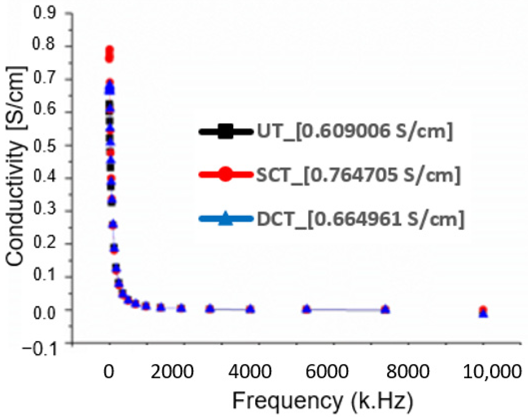
To investigate the effect of cryogenic treatment on the samples, hardness measurement tests and electrical conductivity measurements were performed on the materials before and after the cryogenic treatment. The average hardness measurements of the materials are shown in

Table 4. Average hardness values of the samples.

Materials	Hardness	Units
Untreated	36	HRC
Shallow cryogenic treatment	38
Deep cryogenic treatment	39

and the electric conductivity measurements in Figure 2.

The cryogenic treatment slightly increased the hardness of the samples. The increase in hardness with deep cryogenic treatment depends on the crystallographic and microstructural changes and the fine distribution of microcarbons [29,30]. Figure 2 shows that the highest conductivity value was for the shallow cryogenically treated material, followed by the deep cryogenically treated and untreated material, respectively. This means that the thermal vibrations of the atoms were weakened with the cooling of the metal materials, so the electrical resistance decreased, and the electrical conductivity increased [31].

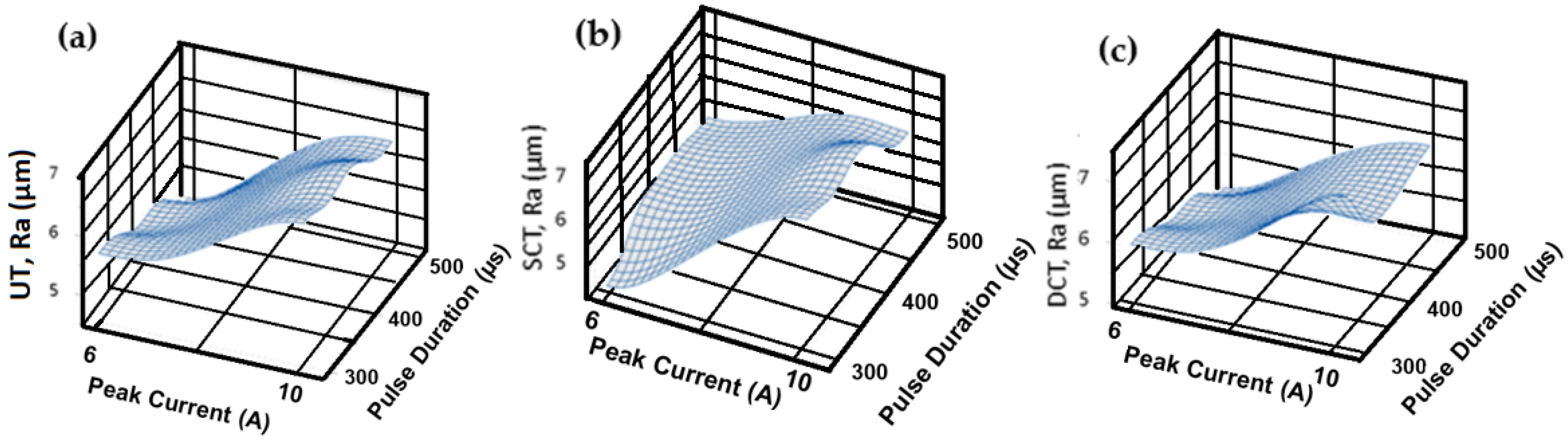
In the EDM tests, an electrolytic copper electrode with a diameter of 18 mm and a density of 8.9 g/cm³ was used (

Table 5. Properties of the electrode material.

	Properties	Values
1	Melting point (°C)	1083
2	Elastic modulus, € (N/mm2)	1.23 × 105
3	Poisson’s ratio	0.26
4	Density (g/cm3)	8.90

). For the experimental study, after consulting the literature, electrical discharge machining was performed with the selected parameters (three different pulse-on times, two peak currents, and fixed pulse-off time and chip depth). The obtained average surface roughness and MRR results were evaluated and are shown in

Table 6. Parameters used in experimental work and experimental results.

Order	Materials	Depth (mm)	Peak Current (A)	Pulse-Off Time (µs)	Pulse-On Time (µs)	Total Processing Time (min)	Ra (µm)	MMR (g)
1	UT	1	10	10	400	22	6.81	2.355
2	DCT		10		300	21	7.35	2.569
3	DCT		6		400	47	5.53	2.116
4	SCT		6		400	46	5.44	2.073
5	UT		10		300	20	6.9	2.272
6	UT		6		300	49	5.64	2.220
7	SCT		6		300	47	4.5	2.147
8	SCT		6		500	47	5.29	2.085
9	UT		10		500	21	6.32	2.265
10	DCT		10		500	23	6.46	2.458
11	UT		6		400	45	5.22	1.950
12	SCT		10		400	18	7.35	1.936
13	DCT		10		400	21	6.22	2.335
14	DCT		6		500	49	5.06	2.464
15	UT		6		500	50	4.61	2.167
16	SCT		10		300	19	7.36	2.222
17	DCT		6		300	47	5.91	2.163
18	SCT		10		500	21	6.28	2.451

. The average surface roughness variations of the UT, SCT and DCT samples at peak current (A) values of 6 and 10 A are shown in Figure 3.

Figure 3 shows that the minimum average surface roughness value was 4.50 μm in the SCT sample at 6 A peak current and 300 μs pulse-on time. The highest average surface roughness value (7.36 μm) was obtained for the factor levels A₂B₂C₁. For MRR, the highest amount of chip removal (2.569 g) was at factor levels A₂B₃C₁, while the lowest amount of chip removal was found to be at A₂B₂C₂. The highest machining time (50 min) was at factor levels A₁B₁C₁, whereas the lowest machining time (18 min) was at A₂B₂C₂. As the amount of current increased, the average surface roughness generally increased, but when the amount of current decreased, the average surface roughness improved. In this case, it can be said that increased peak current reduced the amount of wear, increased the average surface roughness value, but did not greatly affect the MRR. These results are in line with those in the literature. Torres et al. also found that in the processing of titanium diboride material with EDM, the current intensity was effective on the MRR and average surface roughness, but as a result of the melting and evaporation of the material due to the increased heat and current, the MRR increased considerably [32].

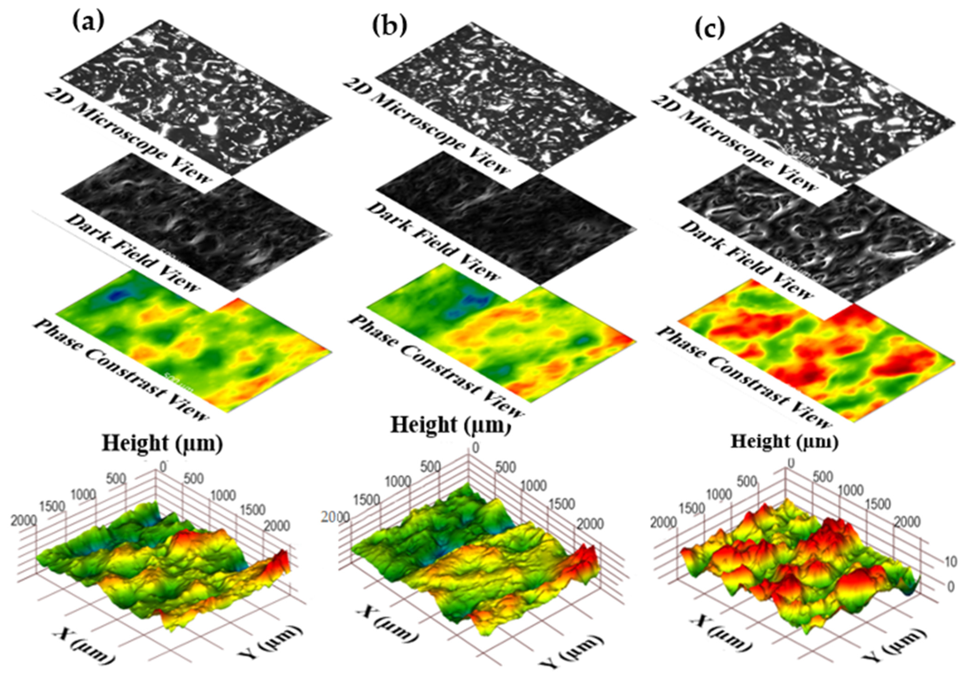
The 3D profilometer, 2D microscopic, dark-field and phase-contrast images used in the analysis of the UT, SCT and DCT sample surfaces are shown in Figure 4. More green parts can be seen in the UT specimens. On the DCT samples, the red regions were observed to increase. In the DCT samples, a large difference in elevation is shown. Dark-field microscopy describes methods in both electron and light microscopy which exclude the unscattered beams from the image. This image provides a simulated dark-field view of the measured sample, as would be obtained by a dark-field microscope. As a result, the field around the specimen is generally dark. In Figure 4, black and white appeared to be more prominent in the DCT sample. This showed that the surface was rougher. The phase-contrast view provides a false color representation of the measured sample. Each color corresponds to a different height. As can be seen from these images, the average surface roughness of the SCT sample was lower.

3.2. Microstructure Analysis

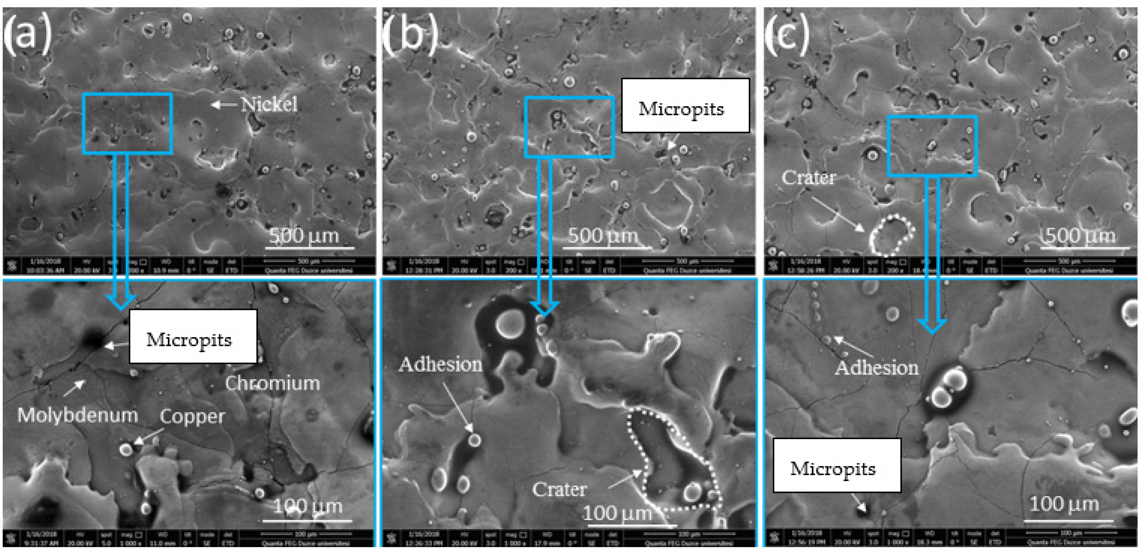
The energy discharged during the EDM process causes very high temperatures to be generated at the spark point. This causes part of the sample surface to evaporate and dissipate. In the process of completing each discharge current, craters, microcracks and spherical particles formed on crater edges can develop in various sizes on the surfaces being processed [33]. The SEM images of the UT, SCT and DCT samples from the experiments resulting in the lowest average surface roughness are shown in Figure 5. Crater formation, adhesions, micropores and copper particles of the electrode material were formed on the surfaces of the UT, SCT and DCT specimens. The higher the current, the higher the discharge energy produced. As a result, damage on the surface of the workpiece caused by a larger crater can be observed [34]. The surfaces were eroded by the smelting process. Moreover, microcracks were more pronounced in the UT specimens. These microcracks are more likely to occur under high energy conditions due to the thermal stress effect on the newly formed layer [32]. Microcracks were seen to decrease in the SCT samples. This is also reflected in average surface roughness values.

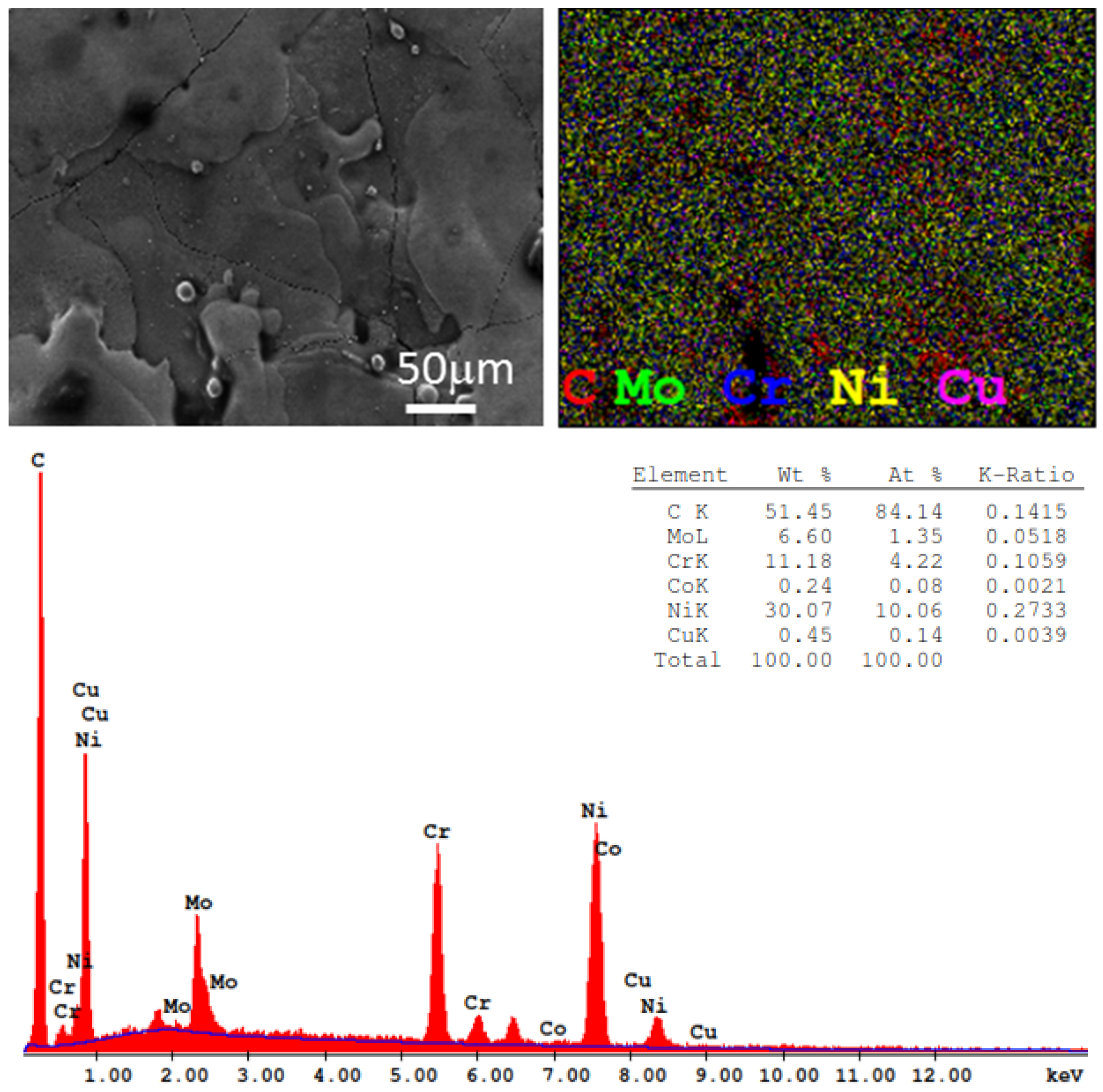
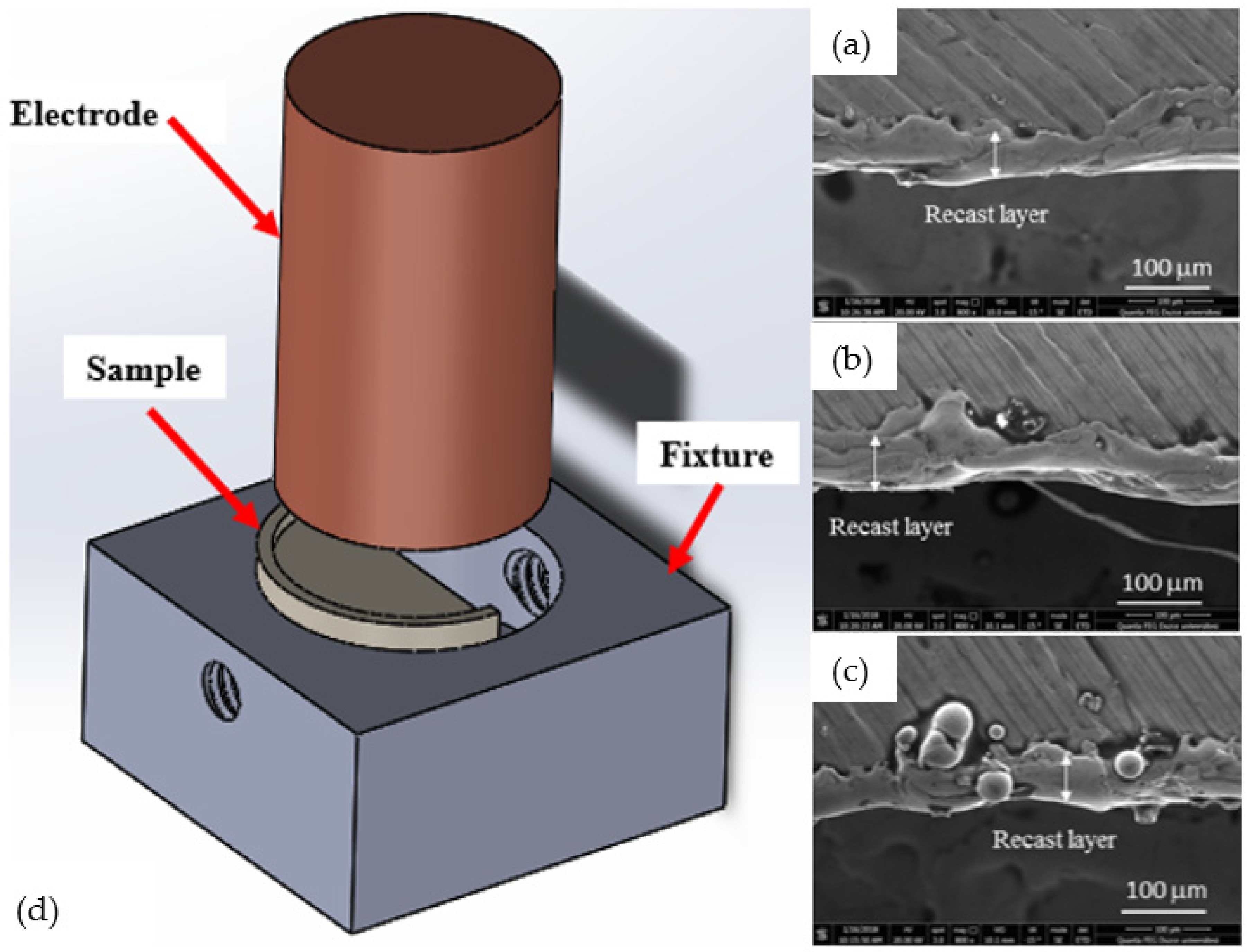
The SEM mapping analysis and the elements in the material obtained from the UT samples used in the experiment are shown in Figure 6. The schematic view and SEM images of processing the materials with the lowest average surface roughness are shown in Figure 7. During the first electron discharge of the electrode, the melted material flowed over the sample surface, forming a thin layer [34]. Since the minimum average surface roughness in UT, SCT and DCT samples was found at a peak current of 6 A, the width of the thin layers formed on their surfaces appears to be similar in dimension.

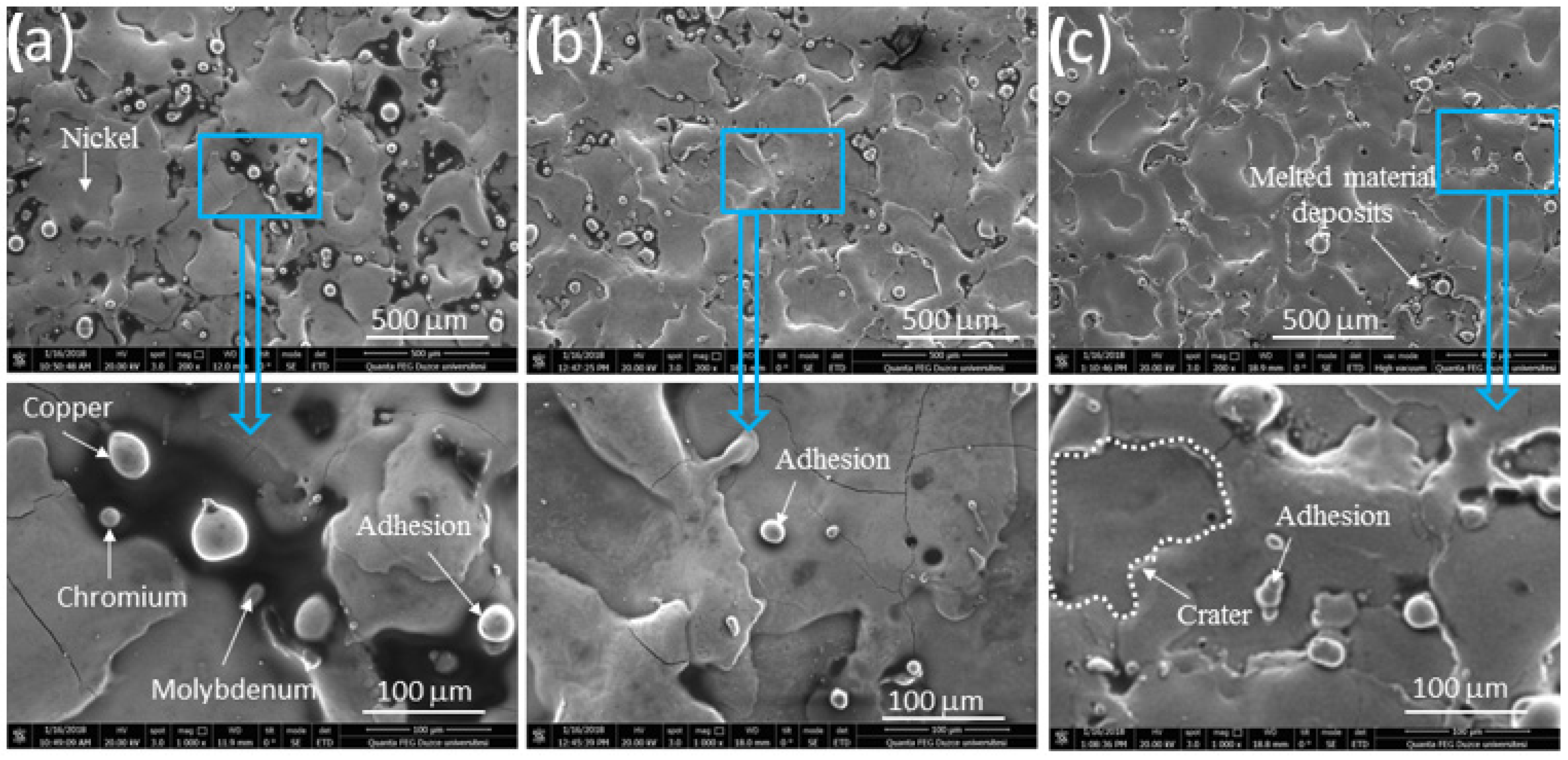
The highest average surface roughness of the UT, SCT and DCT samples was formed at the 10 A peak current. The SEM images of these surfaces are shown in Figure 8. More adhesion particles can be seen on the surface of the UT sample in comparison with those formed on the SCT and DCT samples. More micropits were formed in the UT sample than in the SCT and DCT samples. Craters were formed in the DCT specimens, while the adhesion particles are few in number. It can be said that these differences in the samples were influenced by the cryogenic treatment.

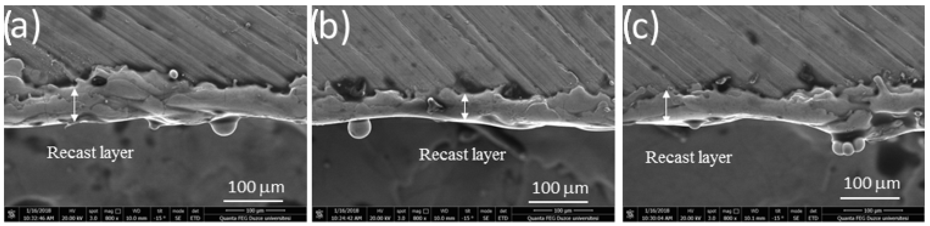
The SEM images of the materials with the highest average surface roughness are shown in Figure 9. During the first electron discharge of the electrode, particles melted from the material surface flow to the sample surface, forming a thin layer. The highest average surface roughness in the UT, SCT and DCT samples was generated at a peak current of 10 A. The width of the thin layers formed on the surface is almost the same in all samples. More spherical particles seemed to adhere in the UT and DCT samples.

3.3. Analysis of the Signal-to-Noise (S/N) Ratio

The interactions of the MRR and Ra results with the control factors were measured by carrying out the experimental design. Signal/noise (S/N) ratios were used in the optimization of the control factors.

Table 7. Input and output parameters of Hastelloy C22 alloy according to L₁₈ orthogonal array.

No	Peak Current (A)	Materials	Pulse-On Time (µs)	Ra (µm)	S/N for Ra	MRR (g/min)	S/N for MRR	Predicted Ra (µm)	S/N for Predicted Ra (µm)	Predicted MRR (g/min)	S/N for Predicted MRR (g/min)
Input				Output Parameters
1	10	UT	400	6.81	−16.662	0.107	19.412	6.70	−16.525	0.103	−19.729
2	10	DCT	300	7.35	−17.325	0.117	18.636	7.38	−17.355	0.120	−18.416
3	6	DCT	400	5.53	−14.854	0.045	26.935	5.36	−14.578	0.048	−26.315
4	6	SCT	400	5.44	−14.712	0.045	26.935	5.51	−14.816	0.037	−28.443
5	10	UT	300	6.9	−16.777	0.114	18.861	7.19	−17.131	0.121	−18.344
6	6	UT	300	5.64	−15.025	0.045	26.935	5.35	−14.570	0.038	−28.404
7	6	SCT	300	4.5	−13.064	0.046	26.744	4.81	−13.646	0.056	−25.036
8	6	SCT	500	5.29	−14.469	0.043	27.330	4.91	−13.823	0.0401	−27.937
9	10	UT	500	6.32	−16.014	0.108	19.331	6.14	−15.760	0.104	−19.592
10	10	DCT	500	6.46	−16.204	0.102	19.828	6.26	−15.934	0.102	−19.802
11	6	UT	400	5.22	−14.353	0.043	27.330	5.33	−14.528	0.046	−26.595
12	10	SCT	400	7.35	−17.325	0.108	19.331	7.28	−17.246	0.115	−18.778
13	10	DCT	400	6.22	−15.875	0.102	19.828	6.39	−16.112	0.098	−20.122
14	6	DCT	500	5.06	−14.083	0.05	26.020	5.26	−14.414	0.049	−26.090
15	6	UT	500	4.61	−13.274	0.043	27.330	4.79	−13.608	0.046	−26.725
16	10	SCT	300	7.36	−17.337	0.17	15.391	7.05	−16.960	0.160	−15.917
17	6	DCT	300	5.91	−15.431	0.046	26.744	5.88	−15.393	0.043	−27.330
18	10	SCT	500	6.28	−15.959	0.117	18.636	6.66	−16.466	0.119	−18.430

shows estimates of the Ra and MRR and the S/N ratios. Estimated values were calculated with the module (fit model) using the program Minitab Normally, both MRR and electrode wear loss are calculated for the abrasion of materials, and the amount of wear is determined with respect to time. As a result of the experiments, the weight of the electrode materials was seen to increase. In this weight increase, chip particles melted from the material surface adhered to the surface of the electrode where it formed a thin film layer.

The most effective parameters in terms of processing time were obtained in the UT samples with 300 μs pulse-on time and 10 A peak current, and in the SCT samples with 500 μs pulse-on time and 10 A peak current, while the most effective parameters in the DCT samples were with 300 μs pulse-on time and 10 A peak current. The difference in the pulse-on time for the SCT samples indicated the effect of shallow cryogenic treatment.

When the results were analyzed via the Taguchi method, the effects of the control factors were seen. The S/N and significance response tables for MRR and average surface roughness are shown graphically in

Table 8. S/N and significance response tables for average surface roughness and MRR.

Average Surface Roughness Ra (µm)				Response Table for Ra Means
Level	Peak Current	Materials	Pulse-On time (µs)	Level	Peak Current	Materials	Pulse-On time (µs)
1	−14.36	−15.35	−15.83	1	5.244	5.917	6.277
2	−16.61	−15.48	−15.63	2	6.783	6.037	6.095
3	-	−15.63	−15.00	3	-	6.088	5.670
Range	2.25	0.28	0.83	Range	1.539	0.172	0.607
Rank	1	3	2	Rank	1	3	2
MRR (g/min)				Response Table for MRR Means
Level	Peak Current	Materials	Pulse-on time (µs)	Level	Peak Current	Materials	Pulse-on time (µs)
1	−26.92	−23.20	−22.22	1	0.04511	0.07667	0.08967
2	−18.81	−22.40	−23.30	2	0.11611	0.08817	0.07500
3	-	−23.00	−23.08	3	-	0.07700	0.07717
Range	8.120	0.81	1.080	Range	0.07100	0.01150	0.01467
Rank	1	3	2	Rank	1	3	2

.

When Table 8 was examined, the most effective parameters observed for the average surface roughness and MRR were A₁B₁C₃ and A₂B₂C₁, respectively.

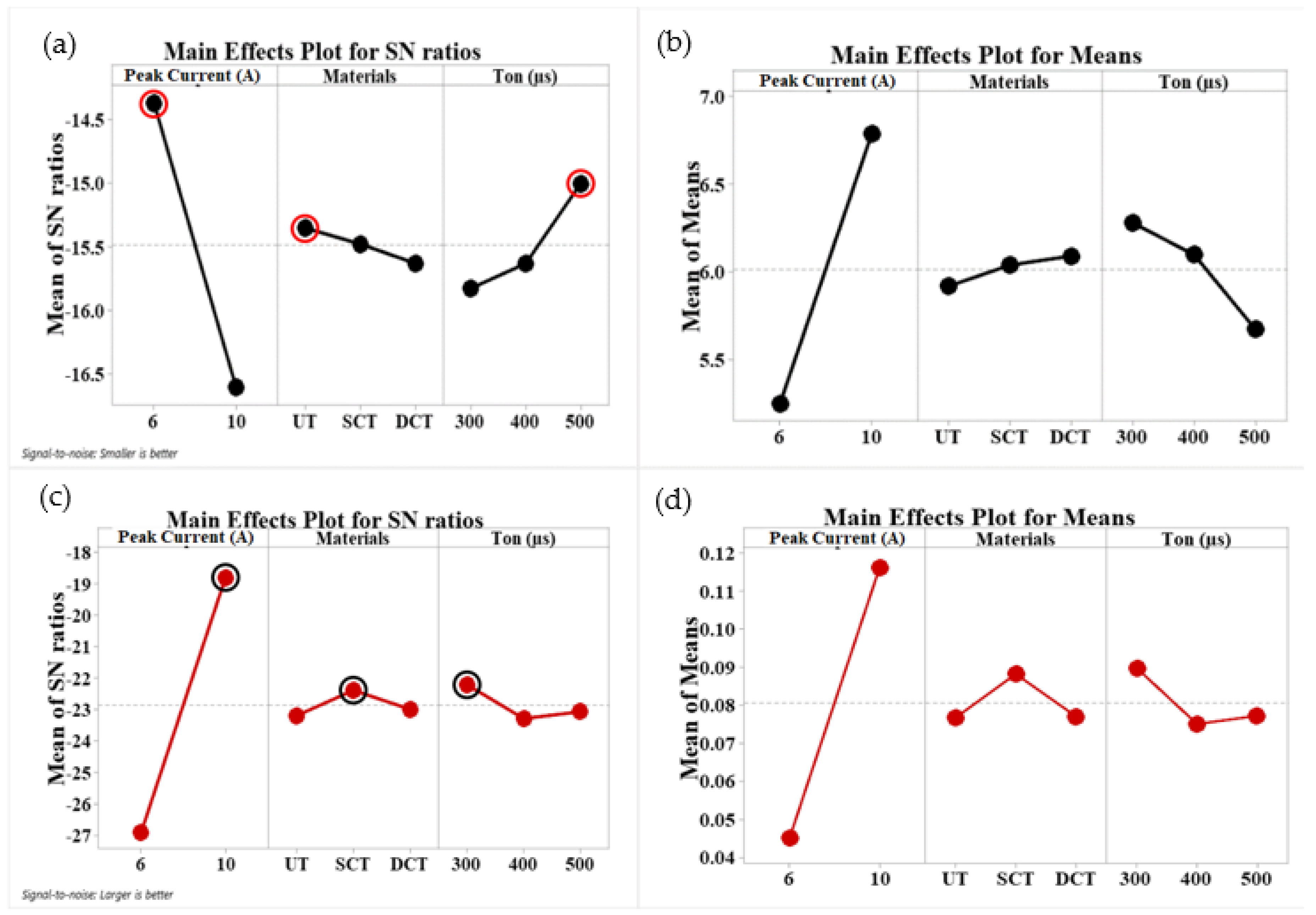
The main effect plots for mean surface roughness and MRR are shown in Figure 10, and the plot of actual values and predicted values is shown in Figure 11. In the main effect plot for average surface roughness, the smallest values are the best. However, in the main effect plot for MRR, the highest values are the best. Accordingly, the optimum values for the average surface roughness were obtained at the A₁B₁C₃ factor levels and the effective values for MRR at the A₂B₂C₁ factor levels.

3.4. ANOVA Analyses

Analysis of variance (ANOVA) is a statistical method used to determine the individual interactions of all control factors in an experimental design. In this study, ANOVA was used to analyze the effects of pulse-on time, materials and peak current on average surface roughness and MRR. This analysis was carried out at a 5% significance level and a 95% confidence level. In ANOVA, the significance of the control factors is determined by comparing the F values of each control factor [34,35,36].

The ANOVA results for the average surface roughness and MRR are shown in

Table 9. ANOVA results for average surface roughness and MMR.

Average Surface Roughness
Source	DF	Seq SS	Contribution %	Adj SS	Adj MS	F-Value	p-Value
Peak current (A)	1	10.6568	74.79	1.13603	1.13603	6.14	0.038
Pulse-on time (µs)	1	1.1041	7.75	0.02373	0.02373	0.13	0.730
Materials	2	0.0931	0.65	0.67839	0.33919	1.83	0.221
Peak current * Pulse-on time	1	0.1776	1.25	0.17763	0.17763	0.96	0.356
Peak current * Materials	2	0.4152	2.91	0.41521	0.20761	1.12	0.372
Pulse-on time * Materials	2	0.3218	2.26	0.32182	0.16091	0.87	0.455
Error	8	1.4798	10.39	1.47975	0.18497
Total	17	14.2484	100.00
R-sq 89.61%				R-sq (adj) 77.93%
Material Removal Rate
Source	DF	Seq SS	Contribution %	Adj SS	Adj MS	F-Value	p-Value
Peak current (A)	1	0.022684	86.43	0.002578	0.002578	17.62	0.003
Pulse-on time (µs)	1	0.000469	1.79	0.000231	0.000231	1.58	0.245
Materials	2	0.000514	1.96	0.000027	0.000013	0.09	0.914
Peak current * Pulse-on time	1	0.000444	1.69	0.000444	0.000444	3.04	0.120
Peak current * Materials	2	0.000603	2.30	0.000603	0.000302	2.06	0.190
Pulse-on time * Materials	2	0.000361	1.38	0.000361	0.000181	1.24	0.341
Error	8	0.001170	4.46	0.001170	0.000146
Total	17	0.026246	100.00
R-sq 95.54%				R-sq (adj) 90.52%

Seq SS: Sequential sum of squares; Adj. SS: adjusted sum of squares; Adj. MS: adjusted mean squares; F: statistical test; P: statistical value. *: multiplication sign

. Peak current was revealed to be the most effective factor for average surface roughness and MRR at 74.79% and 86.43%, respectively. The increase in the amount of peak current affected the wear loss in the positive direction. However, the average surface roughness value was affected negatively.

3.5. Regression Analysis of Average Surface Roughness and MRR

Regression analyses are performed for the modeling and analysis of different variables with a relationship between one dependent variable and one or more independent variables [35]. Linear regression models are relatively simple and provide an easy-to-interpret mathematical formula that can produce predictions. In this study, the equations for estimation of the average surface roughness and MRR were calculated using regression analysis. Equation estimates were made as linear models. Estimated linear equations for the output parameters are shown in

Table 10. Equations for the estimation of average surface roughness and MRR.

Average Surface Roughness
Linear
UT	Ra (μm)	=	4.052 + 0.3847 Peak current − 0.00303 Pulse-on times
SCT	Ra (μm)	=	4.172 + 0.3847 Peak current − 0.00303 Pulse-on times
DCT	Ra (μm)	=	4.224 + 0.3847 Peak current − 0.00303 Pulse-on times
Quadratic
UT	Ra (μm)	=	0.67 + 0.623 Peak current + 0.0106 Ton − 0.000012 Pulse-on times^2 − 0.000608 Peak current * Pulse-on times
SCT	Ra (μm)	=	−1.33 + 0.723 Peak current + 0.0139 Pulse-on times − 0.000012 Pulse-on times^2- 0.000608 Peak Current * Pulse-on times
DCT	Ra (μm)	=	1.66 + 0.538 Peak current + 0.0103 Ton − 0.000012 Pulse-on times^2 −0.000608 Peak current * Pulse-on times
Material Removal Rate
Linear
UT	MRR(g/min)	=	−0.0403 + 0.01775 Peak current − 0.000063 Pulse-on times
SCT	MRR(g/min)	=	−0.0288 + 0.01775 Peak current − 0.000063 Pulse-on times
DCT	MRR(g/min)	=	−0.0400 + 0.01775 Peak current − 0.000063 Pulse-on times
Quadratic
UT	MRR(g/min)	=	−0.016 + 0.02867 Peak current − 0.000450 Pulse-on time + 0.000001 Pulse-on times^2 − 0.000030 Peak current * Pulse-on times
SCT	MRR(g/min)	=	0.002 + 0.03392 Peak Current − 0.000570 Pulse-on times + 0.000001 Pulse-on times^2 − 0.000030 Peak current * Pulse-on times
DCT	MRR(g/min)	=	−0.000 + 0.02717 Peak Current − 0.000458 Pulse-on time + 0.000001 Pulse-on times^2 − 0.000030 Peak current * Pulse-on times

.

3.6. Interval Estimation for Ra and MRR

It was necessary to evaluate whether the system had realized the optimization accurately enough. For this purpose, the following equations were used in the specification of the confidence interval (CI) for estimated Ra and MRR.

Optimal results were obtained using the Taguchi method. The estimated optimum values (Ra and MRR) were calculated using Equations (5) and (6), respectively.

$$R{a}_P=T_{Ra}+(A_1-T_{Ra})+(B_1-T_{Ra})+(C_3-T_{Ra})$$

(5)

$$MR{R}_P=T_{MRR}+(A_2-T_{MRR})+(B_2-T_{MRR})+(C_1-T_{MRR})$$

(6)

where $T_{Ra}$ and $T_{MRR}$ state the average of all values (Ra and MRR) obtained from the experiments. Estimated values were compared with those of the verification experiments to determine the confidence interval (CI). The CI for average surface roughness was calculated using Equations (7) and (8). Estimated values should fall within the confidence interval [36].

Table 11. Confidence interval (CI) formulae symbols [1].

No.	Symbol	Description
1	Fα;1;fe	F ratio at a 95% (at F table)
2	α	Significance level
3	fe	Degrees of freedom of error
4	Ve	Error variance
5	r	Number of replications for confirmation experiment
6	neff	Effective number of replications
7	N	Total number of experiments
8	Tdof	Total main factor degrees of freedom

explains the symbols used in the CI equations: n_eff is the effective number of replications; V_e is error Variance; N is the total number of experiments; and T_dof is the total main factor degrees of freedom; F_α, 1, f_e is the F ratio at a 95% confidence; α is the significance level; f_e is the degrees of freedom of error [37].

$$CI=\sqrt{F_{\alpha ;1;f_e}x{V}_{e}x\left(\frac{1}{n_{eff}}+\frac{1}{r}\right)}$$

(7)

$n_{eff}$ formula:

$$n_{eff}=\frac{N}{1+[T_{dof}]}$$

(8)

The optimal average surface roughness with the CI at 95% was estimated as in Equation (9).

$$\left[\right(T_{Ra}\mathrm{or}{T}_{MRR}\left)\right]-\left[\mathrm{CI}\right]<\left(\mathrm{Ra}\mathrm{or}\mathrm{MRR}\right)\exp <\left[\right(T_{Ra}\mathrm{or}{T}_{MRR}\left)\right]+\left[\mathrm{CI}\right]$$

(9)

5.0781 < Ra_Exp < 6.9479

(10)

0.0544 < MRR_Exp < 0.1068

(11)

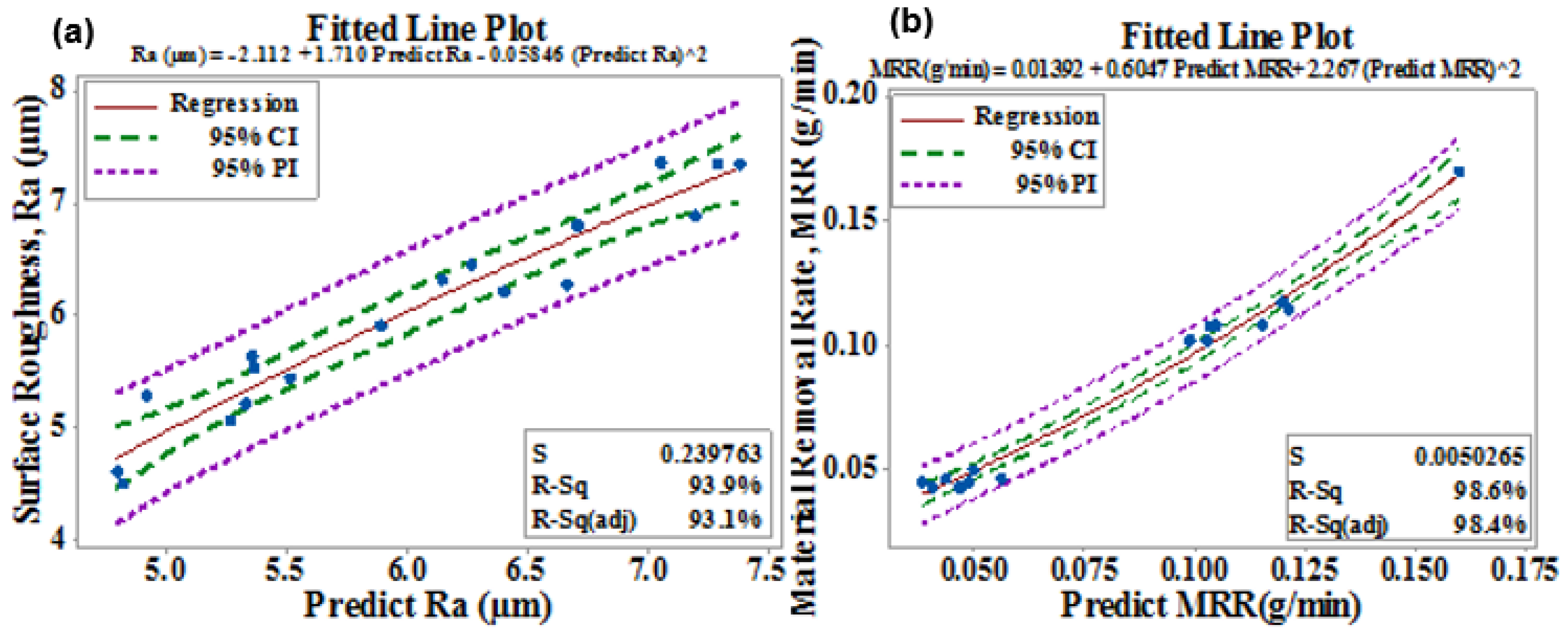
Quadratic regression analysis was then applied to determine whether the predicted values of the experimental results were within the CI. This test was performed to determine the relationship between the predicted values using the Taguchi method and the experimental results. When the results were evaluated, it was found that the estimated values were within the CI limit (95%) in the regression analysis (Figure 11).

3.7. Grey Relational Analysis

Gray correlation analysis, which is one of the multi-factorial decision-making methods, forms gray correlation levels in order to evaluate performance characteristics. The calculation steps of the gray relational analysis method using Equation (10) are as follows.

• Step 1: Order of reference (Ra and MRR) values.

  $$x_0=\left(x_0(1),x_0(2),x_0(3),\dots \dots x_0(n)\right)$$

  (12)
• Step 2: Normalization of the data obtained from the test results.

One of the most commonly used methods in normalization is linear data preprocessing. In considering the normalization of the factor series, one of the criteria (“higher the better”, “lower the better”, “nominal the better” or “best effective”) reflects the characteristic of the series. If the value of the points on the peak is low, it is a desirable feature. The points that receive low values in linear normalization are those close to “1”. Higher value points will have values close to “0”.

The “higher the better” normalization is given in Equation (11).

$$x_i(k)=\frac{x_i^0(k)-\min x_i^0(k)}{\max x_i^0(k)-x_i^0(k)}$$

(13)

$x_i^0\left(k\right)$, i series k. value in the range, $x_i\left(k\right)$ after normalization i. series k. value in the range, $min x_i^0\left(k\right)$ is the minimum value in the i series, max $x_i^0\left(k\right)$ is the maximum value in the i series.

The “lower the better” normalization is given in Equation (12).

$$x_i(k)=\frac{ma{x}_i^0(k)-x_i^0(k)}{\max x_i^0(k)-\min x_i^0(k)}$$

(14)

The “nominal the better” normalization is given in Equation (13).

$$x_i(k)=1-\frac{|x_i^0(k)-x^0|}{(max{x}_i^0(k)-x^0)}$$

(15)

Here, x⁰ represents the desired (best) effective value.

• Step 3: The m series to be compared with the series $x_i$ are defined in Equation (14).

  $$x_i=\left((x^i(1),x^i(2),x^i(3),\dots \dots x^i(n)\right)i=1,2,\dots \dots ,m$$

  (16)
• Step 4:k, Show k. in the row on the n length. $\mathsf{\epsilon }\left(x_0\left(k\right),x_i\left(k\right)\right)$, k. is the gray relational coefficient at the point. Equations are calculated according to Equations (15)–(18).

$$\epsilon \left(x_0(k),x_j(k)\right)=\frac{{\Delta }_{\min }+\xi {\Delta }_{\max }}{{\Delta }_{oi(k)}+\xi {\Delta }_{\max }}$$

(17)

$${\Delta }_{oi}(k)=\left|x_0(k)-x_j(k)\right|$$

(18)

$${\Delta }_{\min }(k)={\min }_j{\min }_k\left|x_0(k)-x_j(k)\right|$$

(19)

$${\Delta }_{\max }={\max }_j{\max }_k\left|x_0(k)-x_j(k)\right|$$

(20)

V_e ξϵ(0, 1) is a coefficient between 0 and 1.

J = 1, 2,…m; k = 1, 2,……n. ξ function, set the difference between ${\Delta }_{oi}$ and ${\Delta }_{max}$.

Studies show that the value of ξ does not affect the ordering after the gray relational degree.

• Step 5: Finally, the gray relational degree is calculated by Equation (19).

  $$\gamma (x_{0,}{x}_i)=\frac{1}{2}{\displaystyle \sum _{k=1}^n\epsilon \left(x_0(k),x_j(k)\right)}$$

  (21)

$\gamma \left(x_0,x_i\right)$ is a measure of the geometric similarity between the x_i series in the gray system and the x₀ reference series. The size of the gray associative level is an indication that there is a strong relationship between x_i and x₀. If the two series are the same, the gray relational level is 1. The gray relational degree indicates how similar the comparison series is to the reference series. If each criterion weight is given, the criterion gray correlation coefficient is multiplied by the weight value for the importance of the criterion and the gray correlation coefficient is found. This is calculated according to Equation (20).

$$\gamma (x_{0,}{x}_i)=\frac{1}{n}{\displaystyle \sum _{k=1}^n\epsilon \left(x_0(k),x_j(k),(w_i(k))\right)}$$

(22)

In the decision-making problem, one of the reference series, the largest, the smallest, and the most effective values for which the criteria are desired is selected. The specified options will be a pointer to the level of catching criteria with the gray relational level. For example, if the highest series of gray correlational grades is chosen, it will be the best decision-making alternative [20].

In EDM, it is desirable that the average surface roughness value of the work surface is low, and that the average material removal rate is high. In this method, while the reference series are being formed, the average surface roughness is best chosen as the lowest. For MRR, it is constructed according to the larger best equality. In calculating the normalization process for the average surface roughness value and material removal rate, Equation (21) and Equation (22) was used, respectively.

$$x_i(1)=\frac{(max{x}_i^0(1)-x_i^0(1))}{(max{x}_i^0(1)-min{x}_i^0(1))}=\frac{7.36-6.81}{7.36-4.5}=0.192$$

(23)

$$x_i(1)=\frac{x_i^0(1)-\min x_i^0(1)}{max{x}_i^0(1)-min{x}_i^0(1)}=\frac{0.107-0.043}{0.170-0.043}=0.503$$

(24)

The results of normalization are subtracted from the reference series and the distance matrix required for the coefficient matrix is found. For the calculation of the coefficient matrix, the mean value x = 0.5 is taken. In order to calculate the average surface roughness and MRR coefficient matrix, Equation (23) and Equation (24) are used.

$${\Delta }_{oi}(k)=\left|x_0(k)-x_j(k)\right|=\left|1-0.192\right|=0.808$$

(25)

$$\epsilon \left(x_0(k),x_j(k)\right)=\frac{{\Delta }_{\min }+\xi {\Delta }_{\max }}{{\Delta }_{oi(k)}+\xi {\Delta }_{\max }}=\frac{0+0.5}{0.808+0.5}=0.382$$

$${\Delta }_{oi}(k)=\left|x_0(k)-x_j(k)\right|=\left|1-0.502\right|=0.498$$

(26)

$$\epsilon \left(x_0(k),x_j(k)\right)=\frac{{\Delta }_{\min }+\xi {\Delta }_{\max }}{{\Delta }_{oi(k)}+\xi {\Delta }_{\max }}=\frac{0+0.5}{0.498+0.5}=0.501$$

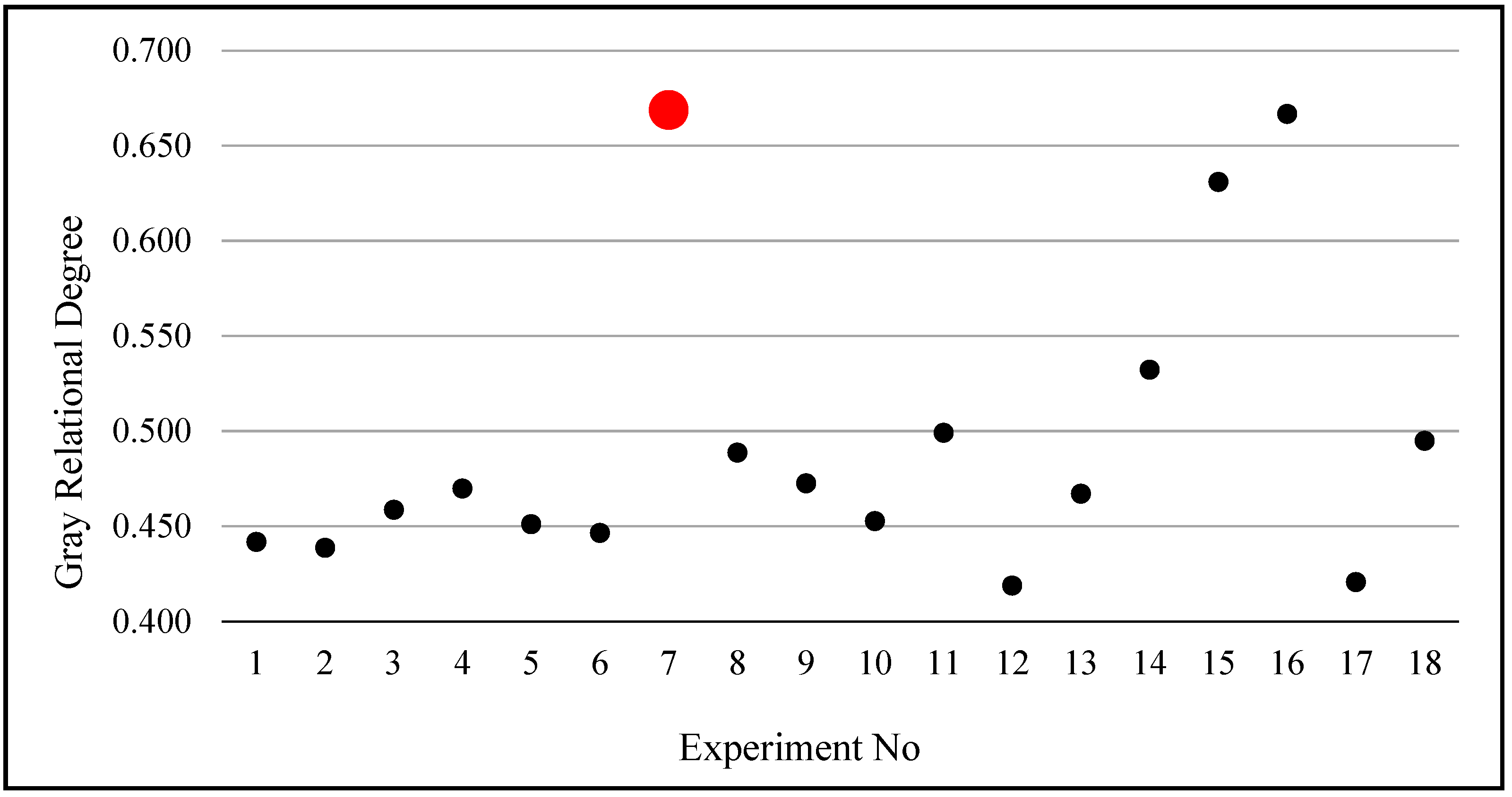
The Microsoft Excel program was used to calculate the normalization of the results obtained from the experiments. The normalization and coefficient matrix values for average surface roughness and MRR are shown in

Table 12. Normalization and coefficient matrix values for average surface roughness and MRR.

Normalization			Coefficient Matrix
Exp No.	Ra	MRR	Exp No.	Ra	MRR
1	0.192	0.503	1	0.382	0.501
2	0.003	0.580	2	0.334	0.543
3	0.639	0.013	3	0.581	0.336
4	0.671	0.014	4	0.603	0.336
5	0.160	0.555	5	0.373	0.529
6	0.601	0.016	6	0.556	0.337
7	1.000	0.019	7	1.000	0.338
8	0.723	0.001	8	0.644	0.333
9	0.363	0.511	9	0.440	0.505
10	0.314	0.466	10	0.421	0.484
11	0.748	0.000	11	0.665	0.333
12	0.003	0.507	12	0.334	0.504
13	0.398	0.459	13	0.453	0.480
14	0.804	0.055	14	0.718	0.346
15	0.961	0.000	15	0.928	0.333
16	0.000	1.000	16	0.333	1.000
17	0.506	0.021	17	0.503	0.338
18	0.377	0.582	18	0.445	0.544

. After finding the average surface roughness and MRR coefficient matrices, the average of the values found gives a gray relational degree. The highest value in the calculated range is defined as the effective value [20,37,38,39,40]. The effective value for this study was in the parameters used in the seventh experiment (

Table 13. Gray associative grades and ordering for average surface roughness and MRR.

Exp No.	Peak Current	Materials	Pulse-On Time (µs)	Ra (µm)	MRR (g)	Gray Degree	Ranking
1	10	UT	400	6.81	0.1070	0.442	15
2	10	DCT	300	7.35	0.1160	0.439	16
3	6	DCT	400	5.53	0.0450	0.459	11
4	6	SCT	400	5.44	0.0450	0.470	9
5	10	UT	300	6.90	0.1130	0.451	13
6	6	UT	300	5.64	0.0450	0.447	14
7	6	SCT	300	4.50	0.0450	0.669	1
8	6	SCT	500	5.29	0.0430	0.489	7
9	10	UT	500	6.32	0.1080	0.473	8
10	10	DCT	500	6.46	0.1020	0.453	12
11	6	UT	400	5.22	0.0430	0.499	5
12	10	SCT	400	7.35	0.1076	0.419	18
13	10	DCT	400	6.22	0.1015	0.467	10
14	6	DCT	500	5.06	0.0500	0.532	4
15	6	UT	500	4.61	0.0430	0.631	3
16	10	SCT	300	7.36	0.1700	0.667	2
17	6	DCT	300	5.91	0.0460	0.421	17
18	10	SCT	500	6.28	0.1170	0.495	6

).

The gray relational degree graph for maximum MRR and minimum average surface roughness values is shown in Figure 12. The top point in the graph shows the effective value to be obtained for both output parameters. The highest MRR was obtained in the SCT samples and was reached at the lower peak current of 6 A. This result can be attributed to the increased electrical conductivity of the sample due to the shallow cryogenic treatment, because the electrical conductivity of the sample affected the EDM performance [14].

4. Conclusions

The conclusions reached from the results of the study on the effects of shallow and deep cryogenic treatment applied to corrosion-resistant superalloys are given below.

• The applied cryogenic treatment increased the hardness of the corrosion-resistant superalloy.
• The highest electrical conductivity value was in the SCT, followed by the DCT and UT materials, respectively.
• The minimum average surface roughness value was 4.50 μm in the SCT sample at 6 A peak current and 300 μs pulse-on time.
• The maximum average surface roughness value was 7.36 μm in the SCT sample at 10 A peak current and 300 μs pulse-on time.
• The highest MRR was 2.569 g in the DCT sample at 10 A peak current and 300 μs pulse-on time.
• The minimum processing time was 18 min for the SCT sample at 10 A peak current and 400 μs pulse-on time.
• The increase in the amount of current affected the wear loss in a positive way, while the average surface roughness value was affected in the negative direction.
• Average surface roughness improved when the flow rate was decreased.
• A thin layer from the workpiece adhered to the surface of the electrode.
• Cryogenic treatment reduced the particles adhering to the sample surface.
• Cryogenic treatment reduced micropores and cracks on the sample surface.
• The most effective factors for average surface roughness and MRR via the Taguchi method were A₁B₁C₃ and A₂B₂C₁, respectively.
• Peak current was the most effective factor for average surface roughness and MRR, at 74.79% and 86.43%, respectively.
• When examined in terms of Taguchi-gray relational degrees, the most effective parameters for both average surface roughness and MRR were the SCT sample, 6 A peak current and 300 μs pulse-on time.

References

- Akincioğlu, S.; Gökkaya, H.; Uygur, İ. The effects of cryogenic-treated carbide tools on tool wear and surface roughness of turning of Hastelloy C22 based on Taguchi method. Int. J. Adv. Manuf. Technol. 2016, 82, 303–314. [Google Scholar] [CrossRef]
- Akincioğlu, S.; Gökkaya, H.; Uygur, İ. A review of cryogenic treatment on cutting tools. Int. J. Adv. Manuf. Technol. 2015, 78, 1609–1627. [Google Scholar] [CrossRef]
- Huang, J.; Zhu, Y.; Liao, X.; Beyerlein, I.; Bourke, M.; Mitchell, T. Microstructure of cryogenic treated M2 tool steel. Mater. Sci. Eng. 2003, 339, 241–244. [Google Scholar] [CrossRef]
- Collins, D.N. Deep Cryogenic Treatment of Tool Steels:A Review. Heat Treat. Met. 1996, 2, 40–42. [Google Scholar]
- Lomte, V.S.; Gogte, L.C.; Peshwe, D. On electrical resistivity of AISI D2 steel during various stages of cryogenic treatment. AIP Conf. Proc. 2012, 1434, 1183–1189. [Google Scholar]
- Collins, D.N. Deep cryogenic treatment of a D2 cold work tool steel. Heat Treat. Met. 1997, 24, 71–74. [Google Scholar]
- Yun, D.; Xiaoping, L.; Hongshen, X. Classic contributions: Cryogenic treatment Deep cryogenic treatment of high speed steel: Microstructure and mechanism. Int. Heat Treat. Surf. Eng. 2008, 2, 80–84. [Google Scholar] [CrossRef]
- Bensely, A.; Venkatesh, S.; Lal, D.M.; Nagarajan, G.; Rajadurai, A.; Junik, K. Effect of cryogenic treatment on distribution of residual stress in case carburized En 353 steel. Mater. Sci. Eng. 2008, 479, 229–235. [Google Scholar] [CrossRef]
- Akincioğlu, G.; Mendi, F.; Çiçek, A.; Akincioğlu, S. Taguchi optimization of machining parameters in drilling of AISI D2 steel using cryo-treated carbide drills. Sādhanā 2017, 42, 213–222. [Google Scholar] [CrossRef] [Green Version]
- Kumar, S.M.; Lal, M.D.; Renganarayanan, S.; Kalanidhi, A. An experimental investigation on the mechanism of wear resistance improvement in cryotreated tool steels. Indian J. Eng. Mater. Sci. 2001, 8, 198–204. [Google Scholar]
- Gill, S.S.; Singh, J.; Singh, R.; Singh, H. Metallurgical principles of cryogenically treated tool steels-a review on the current state of science. Int. J. Adv. Manuf. Technol. 2011, 54, 59–82. [Google Scholar] [CrossRef]
- SreeramaReddy, T.; Sornakumar, T.; VenkataramaReddy, M.; Venkatram, R. Machinability of C45 steel with deep cryogenic treated tungsten carbide cutting tool inserts. Int. J. Ref. Met. Hard Mater. 2009, 27, 181–185. [Google Scholar] [CrossRef]
- Firouzdor, V.; Nejati, E.; Khomamizadeh, F. Effect of deep cryogenic treatment on wear resistance and tool life of M2 HSS drill. J. Mater. Process. Technol. 2008, 206, 467–472. [Google Scholar] [CrossRef]
- Lee, J.; Schafrik, E.; Liang, Y.; Howes, D. Modern Manufacturing, Mechanical Engineering Handbook; CRC Press: Boca Raton, FL, USA, 1999. [Google Scholar]
- Chen, L.S.; Yan, H.B.; Huang, Y.F. Influence of kerosene and distilled water as dielectrics on the electric discharge machining characteristics of Ti–6A1–4V. J. Mater. Process. Technol. 1999, 87, 107–111. [Google Scholar] [CrossRef]
- Abbas, M.N.; Solomon, G.D.; Bahari, F.M. A review on current research trends in electrical discharge machining (EDM). Int. J. Mach. Tool Manu. 2007, 47, 1214–1228. [Google Scholar] [CrossRef]
- Shetty, N.; Herbert, M.A.; Shetty, D.S.; Shetty, R.; Shivamurthy, B. Effect of process parameters on delamination, thrust force and torque in drilling of carbon fiber epoxy composite. Res. J. Recent Sci. 2013, 2, 47–51. [Google Scholar]
- Bilge, T.; Motorcu, R.A.; Ivanov, A. Optimization of drilling parameters for dimensional accuracy in drilling of compact laminate composite using gray relational analysis. SDU Int. J. Technol. Sci. 2017, 9, 1–22. [Google Scholar]
- Lin, L.J.; Lin, L.C. The use of the orthogonal array with grey relational analysis to optimize the electrical discharge machining process with multiple performance characteristics. Int. J. Mach. Tool Manu. 2002, 42, 237–244. [Google Scholar] [CrossRef]
- Wang, Z.; Zhu, L.; Wu, H.J. Grey relational analysis of correlation of errors in measurement. J. Grey Syst. 1996, 8, 73–78. [Google Scholar]
- Rengasamy, N.; Rajkumar, M.; Kumaran, S.S. An analysis of mechanical properties and optimization of EDM process parameters of Al 4032 alloy reinforced with Zrb2 and Tib2 in-situ composites. J. Alloys Compd. 2016, 662, 325–338. [Google Scholar] [CrossRef]
- Rahul, C.; Datta, S. Electrical discharge machining performance of deep cryogenically treated ınconel 825 superalloy: Emphasis on surface integrity. Metallogr. Microstruct. Anal. 2019, 8, 212–225. [Google Scholar] [CrossRef]
- Kumar, S.; Batish, A.; Singh, R.; Bhattacharya, A. Effect of cryogenically treated copper-tungsten electrode on tool wear rate during electro-discharge machining of Ti-5Al-2.5Sn alloy. Wear 2017, 386–387, 223–229. [Google Scholar] [CrossRef]
- Jaspreet, S.; Mukhtiar, S.; Harpreet, S. Analysis of machining characteristics of cryogenically treated die steels using EDM. Int. J. Mod. Eng. Res. 2013, 3, 2249–6645. [Google Scholar]
- Abdulkareem, S.; Khan, A.A.; Konneh, M. Cooling effect on electrode and process parameters in EDM. Mat. Manuf. Process. 2010, 25, 462–466. [Google Scholar] [CrossRef]
- Ho, K.; Newman, T.S. State of the art electrical discharge machining (EDM). Int. J. Mach. Tool Manu. 2003, 43, 1287–1300. [Google Scholar] [CrossRef]
- Nas, E.; Gökkaya, H. Experimental and Statistical Study on Machinability of the Composite Materials with Metal Matrix Al/B4C/Graphite. Metall. Mat. Trans. A 2017, 48, 5059–5067. [Google Scholar] [CrossRef]
- Zhang, Z.J.; Chen, C.J.; Kirby, D.E. Surface roughness optimization in an end-milling operation using the Taguchi design method. J. Mater. Process. Technol. 2007, 184, 233–239. [Google Scholar] [CrossRef]
- Nanesa, G.H.; Jahazi, M.; Naraghi, R. Martensitic transformation in AISI D2 tool steel during continuous cooling to 173 K. J. Mater. Sci. 2015, 50, 5758–5768. [Google Scholar] [CrossRef]
- Masmiati, N.; Sarhan, A.A. Optimizing cutting parameters in inclined end milling for minimum surface residual stress–Taguchi approach. Measurement 2015, 60, 267–275. [Google Scholar] [CrossRef]
- Jiao, X.; Li, L.; Liu, H.; Yang, K. Mechanical properties of low density alloys at cryogenic temperatures. AIP Conf. Proc. 2006, 824, 69–76. [Google Scholar]
- Torres, A.; Luis, J.C.; Puertas, I. EDM machinability and surface roughness analysis of TiB2 using copper electrodes. J. Alloys Compd. 2017, 690, 337–347. [Google Scholar] [CrossRef]
- Kumar, A.; Kumar, V.; Kumar, J. Investigation of microstructure and element migration for rough cut surface of pure titanium after WEDM. Int. J. Microstruct. Mater. Prop. 2013, 8, 343–356. [Google Scholar] [CrossRef]
- Rajesha, S.; Sharma, K.A.; Kumar, P. On Electro Discharge Machining of Inconel 718 with Hollow Tool. J. Mater. Eng. Perform. 2012, 21, 882–891. [Google Scholar] [CrossRef]
- Sudheer, M.; Prabhu, R.; Raju, K.; Bhat, T. Modeling and analysis for wear performance in dry sliding of Epoxy/Glass/PTW composites using full factorial techniques. ISRN Tribol. 2013, 2013, 624813. [Google Scholar] [CrossRef] [Green Version]
- Cetin, H.M.; Ozcelik, B.; Kuram, E.; Demirbas, E. Evaluation of vegetable based cutting fluids with extreme pressure and cutting parameters in turning of AISI 304L by Taguchi method. J. Clean. Prod. 2011, 19, 2049–2056. [Google Scholar] [CrossRef]
- Kıvak, T. Optimization of surface roughness and flank wear using the Taguchi method in milling of Hadfield steel with PVD and CVD coated inserts. Measurement 2014, 50, 19–28. [Google Scholar] [CrossRef]
- Aslantaş, K.; Ekici, E.; Çiçek, A. Optimization of process parameters for micro milling of Ti-6Al-4V alloy using Taguchi-based gray relational analysis. Measurement 2018, 128, 419–427. [Google Scholar] [CrossRef]
- Muralidharan, B.; Chelladurai, H.; Subbu, K.S. Investigation of magnetic field and shielding gas in electro-discharge deposition process. Proc. IMechE Part C J. Mech. Eng. Sci. 2019, 233, 3701–3716. [Google Scholar] [CrossRef]
- Kara, F. Optimization Of Surface Roughness in Finish Milling of AISI P20+S Plastic-Mold Steel. Mat. Technol. 2018, 52, 200. [Google Scholar] [CrossRef]
Figure 1.
Cryogenic treatment schedule.
Figure 2.
Electrical conductivity of UT (untreated), SCT (shallow cryogenically treated) and DCT (deep cryogenically treated) samples.
Figure 3.
Graphs of average surface roughness variations in materials: (a) UT, (b) SCT and (c) DCT.
Figure 4.
Surface images of the samples: (a) UT (500 µs-6 A), (b) SCT (300 µs-6 A), (c) DCT (500 µs-6 A).
Figure 5.
Microstructure images of samples: (a) UT (1-3), (b) SCT (2-1) and (c) DCT (3-3).
Figure 6.
EDX and imaging mapping analysis, UT-500 µs-6 A.
Figure 7.
Cross-section microstructure images of samples: (a) UT (1-3), (b) SCT (2-1), (c) DCT (3-3) and (d) fixture.
Figure 8.
SEM images of samples: (a) UT (1-7), (b) SCT (2-7) and (c) DCT (3-7).
Figure 9.
Cross-section views of samples: (a) UT (1-7), (b) SCT (2-7) and (c) DCT (3-7).
Figure 10.
Main effects plot and S/N ratio for (a,b) average surface roughness and (c,d) MRR.
Figure 11.
Comparison of predicted values and experimental results for output parameters: (a) average surface roughness, (b) MRR. (CI: confidel interval, PI: predict interval).
Figure 12.
Gray correlation level for lowest average surface roughness and highest MRR.