Autonomous Mobile Robot Implemented in LEGO EV3 Integrated with Raspberry Pi to Use Android-Based Vision Control Algorithms for Human-Machine Interaction ^†

Abstract

Robotic applications, such as educational programs, are well-known. Nonetheless, there are challenges to be implemented in other settings, e.g., mine detection, agriculture support, and tasks for industry 4.0. The main challenge consists of robotic operations supported by autonomous decision using sensed-based features extraction. A prototype of a robot assembled using mechanical parts of a LEGO MINDSTORMS Robotic Kit EV3 and a Raspberry Pi controlled through servo algorithms of 2D and 2D1/2 vision approaches was implemented to tackle this challenge. This design is supported by simulations based on image, position, and a hybrid scheme for visual servo controllers. Practical implementation is operated using navigation guided by running up image-based visual servo control algorithms embedded in a Raspberry Pi that uses a control criterion based on error evolution to compute the difference between a target and sensed image. Images are collected by a camera installed on a mobile robotic platform manually and automatically operated and controlled using the Raspberry Pi. An Android application to watch the images by video streaming is shown here, using a smartphone and a video related to the implemented robot’s operation. This kind of robot might be used to complete field reactive tasks in the settings mentioned above, since the detection and control approaches allow self-contained guidance.

1. Introduction

Robots are one of the most promising devices to be potentially used in industry, agriculture [1,2], medicine [3], education [4,5] and some other fields. These can be programmed, configured, and optimized to perform tasks with high accuracy and great flexibility due to their kinematical degrees of freedom and versatility of adapting tools such as sensors, cameras, and other periphery devices. For instance, robots reach up to places inaccessible to humans, perceiving their surroundings, and collecting information to make decisions by themselves through decision support systems based on artificial intelligence techniques to adapt their movements depending on the requirements. Robots can perceive their surroundings by using several types of sensors, such as cameras, which allows the robot to have human-like perception.

Different configurations of integrated robots applying mobile or fixed cameras or sensors are reported in literature [3,6,7]. These are well-known as visual servoing, which is used to obtain the necessary data of the surroundings from a camera through images locally or remotely collected, by using various kinds of controllers such as task function [8,9,10], predictive control [11,12], rational systems and LMIs (Linear Matrix Inequalities) [13], applying Kalman filters [6], etc. The main goal of visual servo control is to allow the robotic system operation under surrounding changes, detected through the images recorded by a camera to perform tasks according to the decision of a controller. Usually, controllers can be carried out in two ways: the first uses a central station to process images and compute and transmit the controller’s decision to the robot; and the second, the robot performs all tasks. For the last one, the robot’s devices should have an adequate processing capability to process the image and run up as quickly as possible the control algorithms.

Applications use image processing, robotics, and control theory jointly to command the motion of a robot depending on the visual information extracted from the images captured by one or several cameras. Currently, there are many problems of great interest to the scientific community such as different image features extraction of more complex geometries, enhancement of velocity of algorithms, convergence problem in control, and others [14].

Regarding the state of the art, robotic and visual control converges in recent reported topics are related to omnidirectional platforms designed to cooperative robotic systems [15] to make a task. As an example, elements like Raspberry Pi with an integrated camera for image processing and future extraction [16], both operating in the same programing environment were used as mechanism of a manipulative robot. Moreover, an eye-in-hand manipulative robot using optimal controller allows to minimize the force and torque in the joint engines of the robotic systems to assess the performance of the controller [17].

Following the state of the art in robotic systems and its relationship with controllers, in this research work a novel robotic system integrated with technologies with different operating systems is presented, such as the LEGO Educational Kit and the Raspberry Pi to assess visual control algorithms. In addition, an Android application is added for human-machine interaction that allows to visualize the robot’s perspective, thus allowing manual or automatic control of the robot for safe operation in case of being executed in a hostile environment.

This work shows the design of robotic systems either using IBVSs (Image-Based Visual Servo) (see a previous work reported by some authors in [18], PBVSs (Position-Based Visual Servo), or hybrid HBVS (Hybrid-Based Visual Servo) scheme (image and position-based). A camera mounted on the robot can roll over its axis minimizing the non-holonomy of the robotic system [19]. Algorithms are implemented by running up embedded servo-algorithms in open-source platforms. In this case, a Single Board Computer (SBC) known as Raspberry Pi is used. This paper shows a robot assembled as a three degree of freedom (3 DOF) structure using LEGO™ Mindstorms robotic kit, adding a platform to hold a camera. Two of the 3 DOF were used for the platform movement in the XY plane, and the third-degree to enable the platform’s rotation. This proposed robot was implemented as an IBVS and assisted with an Android smartphone for remote operation. One of the main challenges reported in the literature consists of using Mindstorms in other applications beyond educative programs since there are no limitations and impediments [4,20]. These can be jointly configured with other operative systems like Raspbian, Linux, and mobile Android to support open-source codes and other sensors [21,22]. This work is a proposal to explore this challenge focused on algorithms for feature extraction using IBVS, PBVS, and hybrid schemes implemented with an open-source operative system, as the first step of prototypes design to be used in broader applications in real environments.

This paper is organized into five sections. In the second section, a kinematic model of the 3 DOF’s robot, and the image representation using matrix formulation, followed by the equations to design controllers based on the IBVS, PBVS algorithms, and hybrid approach are presented. The third section is related to the experimental setup of assembling the robot, the communication system between the Raspberry Pi, the Mindstorms control and power station Lego EV3 brick, and the mobile interface designed in an Android smartphone. In the fourth section, the simulation results of the IBVS and PBVS algorithms and a hybrid scheme are presented, applied to the proposed 3 DOF robotic system in terms of the image and position error evolution and the robot’s expected poses. Finally, the article shows the results of the implementation using the servo control algorithm IBVS embedded on the Raspberry Pi to recognize a target image remotely monitored by a video streaming application running up in the interface of the Android smartphone.

2. Kinematical Degrees of Freedom Model, and Controller’s Design

In this section, the robotic system is kinematically modeled using position and rotation equations, relating them to the images by using a matrix formulation. These equations are used to design controllers based on application of IBSV, PBVS algorithms, and a hybrid (HBVS) scheme.

2.1. Kinematic Model

This robot can be modeled using a Hilare-type approach implemented with one motor that controls each robot side as shown in Figure 1. This robot kind has reliable performance, low rotation radius, and is easily controllable and simple to assemble [20]. Furthermore, it has three degrees of freedom (3 DOF), two of them make up the XY plane (two degrees of freedom), where the pair (x,y) is the robot’s position in global coordinates used as a reference for the linear displacement assuming linear speed. The other coordinate is related with the z-axis, assigned to any rotation θ around itself.

Using these coordinates, the robot kinematic can be depicted by Equations (1) and (2):

$$\left[\begin{array}{c}\begin{array}{c}\dot{x}\\ \dot{y}\\ \dot{\theta }\end{array}\\ {\dot{\theta }}_{pl}\end{array}\right]=\left[\begin{array}{c}\begin{array}{c}\cos \theta \\ \sin \theta \\ 0\end{array}\\ 0\end{array}\begin{array}{c}\begin{array}{c}0\\ 0\\ 1\end{array}\\ 0\end{array}\begin{array}{c}\begin{array}{c}0\\ 0\\ 0\end{array}\\ 1\end{array}\right]\left[\begin{array}{c}v\\ \omega \\ {\omega }_{pl}\end{array}\right]$$

(1)

$$\left[\begin{array}{c}\dot{x}\\ \dot{y}\\ \begin{array}{c}\dot{\theta }\\ {\dot{\theta }}_{pl}\end{array}\end{array}\right]=\left[\begin{array}{ccc}\frac{r}{2}\cos \theta & \frac{r}{2}\cos \theta & 0\\ \frac{r}{2}\sin \theta & \frac{r}{2}\sin \theta & 0\\ r/L& -r/L& 0\\ 0& 0& 1\end{array}\right]\left[\begin{array}{c}{\omega }_{right}\\ {\omega }_{left}\\ {\omega }_{pl}\end{array}\right]$$

(2)

Equation (1) is a rotation matrix that models linear speed, and robot rotation concerning coordinates axes, and Equation (2) models the angular speed of the robot’s wheels, so both equations can configure a real application. In Equation (1), $\dot{x}$ and $\dot{y}$ are the linear speeds of the robot related to x and y coordinates, and $\dot{\theta }$ is the angular speed related to the rotation movement around z. The term ${\dot{\theta }}_{pl}$ is the orientation related to the camera movements mounted on top of a rotary platform, so this is the third degree of freedom. The relationship between outputs and angular speeds (${\omega }_{right}$, ${\omega }_{left},$ and ${\omega }_{pl}$) of the robot’s wheels are given by Equation (2) [10,20,21]. These are the real inputs of the robotic system modeled for the application implemented here where $r$ is the wheels’ radius,$L$, distance between wheels, ${\omega }_{right}$, right wheel angular speed, and ${\omega }_{left},$ left wheel angular speed.

On the other hand, a mobile robot model can be described in different reference frames. These frames can be the world frame reference or the actuator frame reference. In this proposed robot, the actuator or element that gives a surrounding perception is a camera. Then, to pass from the world’s frame to the image’s frame, it is necessary to transform all frames that pass through the world’s frame, mobile’s frame, and then to the platform’s frame, until the camera’s frame that uses coordinates transformations. This kind of transformation is obtained through the following expressions shown in Equations (3) and (4) [10,15]:

$$\left[\begin{array}{c}\begin{array}{c}{V}_{x_c}\\ V_{y_c}\\ V_{z_c}\end{array}\\ {\mathsf{\Omega }}_{x_c}\\ {\mathsf{\Omega }}_{y_c}\\ {\mathsf{\Omega }}_{z_c}\end{array}\right]=\left[\begin{array}{ccc}0& 0& 0\\ -\sin {\theta }_{pl}& x_c+x_p\cos {\theta }_{pl}& x_c\\ \cos {\theta }_{pl}& -y_c+y_p\sin {\theta }_{pl}& -y_c\\ 0& -1& -1\\ 0& 0& 0\\ 0& 0& 0\end{array}\right]\left[\begin{array}{c}v\\ \omega \\ {\omega }_{pl}\end{array}\right]$$

(3)

where $x_c$ is the x component of the translational vector to pass from platform frame reference to camera frame reference; $x_p,$ the x component of the translational vector to pass from robot frame reference to platform frame reference; $y_c,$ the y component of the translational vector to pass from platform frame reference to camera frame reference; and $y_p$, is the y component of the translational vector to pass from robot frame reference to platform frame reference. $V_{x_c}$, $V_{y_c},$ and $V_{z_c}$ are the linear speeds expressed in the camera’s frame, and ${\mathsf{\Omega }}_{x_c}$, ${\mathsf{\Omega }}_{y_c}$, and ${\mathsf{\Omega }}_z$ are the angular speeds expressed in the camera’s frame.

In this case, a control signal should be applied to change the angular speed of the wheels, then it is necessary to use Equation (2) instead of (1) for the coordinate’s transformation, to obtain an expression for the angular speed of the robot in the camera frame reference [10,22]:

$$\left[\begin{array}{c}\begin{array}{c}{V}_{x_c}\\ V_{y_c}\\ V_{z_c}\end{array}\\ {\mathsf{\Omega }}_{x_c}\\ {\mathsf{\Omega }}_{y_c}\\ {\mathsf{\Omega }}_{z_c}\end{array}\right]=\left[\begin{array}{ccc}0& 0& 0\\ \frac{r\left(x_c+x_p\cos {\theta }_{pl}\right)}{L}-\frac{r\left(\sin {\theta }_{pl}\right)}{2}& \frac{r\left(\sin {\theta }_{pl}\right)}{2}-\frac{r\left(x_c+x_p\cos {\theta }_{pl}\right)}{L}& \frac{x_c}{1}\\ \frac{r\left(\cos {\theta }_{pl}\right)}{2}+\frac{r\left(y_c+y_p\sin {\theta }_{pl}\right)}{L}& \frac{r\left(\cos {\theta }_{pl}\right)}{2}+\frac{r\left(y_c+y_p\sin {\theta }_{pl}\right)}{L}& -\frac{y_c}{1}\\ -\frac{r}{L}& \frac{r}{L}& -\frac{1}{1}\\ 0& 0& 0\\ 0& 0& 0\end{array}\right]\left[\begin{array}{c}{\omega }_{right}\\ {\omega }_{left}\\ {\omega }_{pl}\end{array}\right]$$

(4)

To model the image in the camera, the next subsection will show the equations for the image representation in this frame of reference.

2.2. IBVS Interaction Matrix

Until now, an expression has been obtained that represents a change in the world’s frame into the camera’s frame as shown in Equation (4), nonetheless, it is necessary to find an expression that represents the changes in the camera’s frame into the image (object) frame.

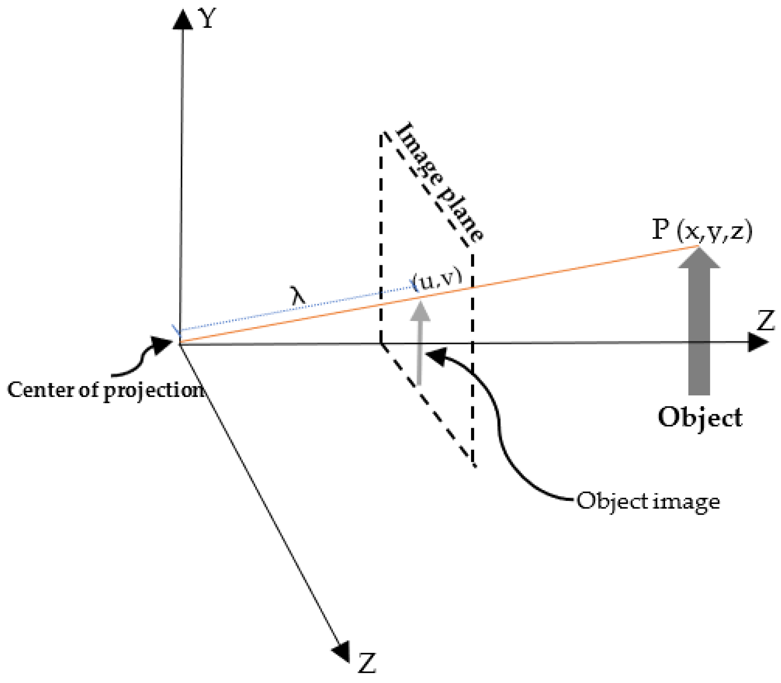
The object image representations are often modeled by the pinhole lens approach as shown in Figure 2. With this approach, the lens is considered an ideal pinhole. The pinhole is located at the lens focal center, and placed behind the image plane to simplify the model. Light passes through this pinhole intersecting the image plane. Thus, P is a point in the world with coordinates x,y,z; and p denotes the projection of P onto the image plane with coordinates (u,v,λ).

Here, the Jacobian Image L_i(s), also called interaction matrix, is used to represent the relative changes in the image into the camera reference frame. Assuming that the image geometry can be modeled using perspective projection and the camera lens is a pinhole type, the following expression can be used [10,20,21]:

$$L_i\left(s\right)=\left[\begin{array}{ccc}-\frac{\lambda }{z_c}& 0& \frac{u}{z_c}\\ 0& -\frac{\lambda }{z_c}& \frac{v}{z_c}\end{array}\begin{array}{ccc}\frac{uv}{\lambda }& \frac{{\lambda }^2+v^2}{\lambda }& v\\ v\frac{{\lambda }^2+v^2}{\lambda }& -\frac{uv}{\lambda }& -u\end{array}\right]$$

(5)

where $\lambda$ is the focal lens distance, and the pair (u,v) are the pixel location. s is a set of visual features extracted from the object.

2.3. PBVS Interaction Matrix

PBVS is aimed to regulate the error between current camera pose and goal pose with respect to the objective. Pose is defined as $\left[\begin{array}{c}X{\left(t\right)}^T\\ U{\theta }^T\end{array}\right]$, where $X\left(t\right)ϵ{ℝ}^{3x1}$ is the translational distance expressed in world frame reference and $U\theta ϵ{ℝ}^{3x1}$ is the rotation angle around the axis defined by the unitary vector $U$, where $U$ represents the orientation vector where the robot is rotating. The interaction matrix is given by [23,24,25]:

$$L_p\left(s\right)=\left[\begin{array}{cc}-I_3& {\left[X\left(t\right)\right]}_x\\ 0_{3x3}& L_{U\theta }\end{array}\right]$$

(6)

where ${\left[X\left(t\right)\right]}_x$ is the skew matrix of X(t) and $L_{\theta u}$ is given by:

$$L_{U\theta }=I_3-\frac{\theta }{2}{\left[U\right]}_x+\left(1-\frac{\mathrm{s}\mathrm{i}\mathrm{n}c\theta }{\mathrm{s}\mathrm{i}\mathrm{n}{c}^2\frac{\theta }{2} }\right){\left[U\right]}_x^2$$

(7)

The kinematic screw describes the changes of the kinematic chain concerning time, also known as Jacobian robot. At this point, it is possible to represent how the image changes depending on the robot movements in the world frame. The following subsection uses the kinematic screw and the interaction matrix to impose an error performance.

2.4. IBVS Servocontrollers

The Image–Based Visual Servo Control (IBVS) scheme uses a set of points that represent visual features of the objective obtained by the camera (real image). The image features (m) are often measured in pixel units and represent a set of image points in image coordinates. The objective image ($s^{*}$) can be static or dynamic. In this research work, it is assumed to be fixed to the world’s frame.

The control scheme is obtained from an error function, and it is computed from the real image and the objective. Thus, the basic equation for an IBVS control scheme is:

$$e_i\left(t\right)=C\left(s\left(t\right)-s^{*}\left(t\right)\right)$$

(8)

where C is the combination matrix, $s\left(t\right)$, a set of visual points in the image plane, and $s^{*}\left(t\right)$, the visual goal feature points. To ensure the convergence of e(t) to zero, a decreasing behavior on the error is imposed:

$${\dot{e}}_i\left(t\right)=-\beta e_i\left(t\right)$$

(9)

where, $\beta$ is a positive gain scalar ($\beta$> 0) representing the time constant of the error convergence. Then, by deriving Equation (8) and equalizing with (9) the relationship between $\beta$ and the error $e_i\left(t\right)$ is obtained:

$$\dot{s}\left(t\right)=-\beta e_i\left(t\right)$$

(10)

As $s\left(t\right)$ represents the visual features, we have an expression to represent changes in the image frame into other frameworks, thus, the chain rule over (10) is allowed to apply as [21]:

$$\dot{s}\left(t\right)=\frac{\partial s\left(t\right)}{\partial r}\frac{\partial r\left(t\right)}{\partial p}\dot{p}$$

(11)

where $r$ is the robot frame and $\dot{p}:{\left[v\omega {\omega }_{pl}\right]}^T$ is the control signal. $\frac{\partial s\left(t\right)}{\partial r}$ represents the image changes into the first robot frame, or the interaction matrix $L\left(s\right)$ described in the last subsection; and $\frac{\partial r\left(t\right)}{\partial p}$ represents the robot changes regarding a known input variable or the Jacobian robot $J_r\left(p\right)$.

Finally, Equation (11) can be rewritten in terms of interaction matrix, well-known as L(s) or Jacobian, and Jacobian robot $J_r\left(p\right)$ as shown:

$$\dot{s}\left(t\right)=L\left(s\right)J_r\left(p\right)\dot{p}$$

(12)

Based on the equality from (10) and (8) the control law is obtained as:

$$-\beta e_i\left(t\right)=L\left(s\right)J_r\left(p\right)\dot{p}$$

(13)

$$\dot{p}=-\beta e_i\left(t\right){\left(L\left(s\right)J_r\left(p\right)\right)}^{+}$$

(14)

where ${\left(L\left(s\right)J_r\left(p\right)\right)}^{+}$ is the pseudo-inverse of $L\left(s\right)J_r\left(p\right)$.

To ensure stability in the sense of Lyapunov, it is proposed as a candidate, the Lyapunov function or quadratic function of the error:

$$V\left(e_i\right)=\frac{1}{2}{\Vert e_i\left(t\right)\Vert }^2$$

(15)

Since the proposed Lyapunov function depends on the quadratic norm of the error, then it can be demonstrated that $\forall e\left(t\right)$,$V\left(e_i\right)\ge 0$ so, the function is positively defined. Now, it is necessary that $\dot{V}\left(e_i\right)\le 0$, then by deriving Equation (15) and replacing on (12) the following expression can be obtained:

$$\dot{V}\left(e_i\right)=-\beta e_i{\left(t\right)}^T\left(L\left(s\right)J_r\left(p\right)\right){\left(L\left(s\right)J_r\left(p\right)\right)}^{+}{e}_i\left(t\right)$$

(16)

to ensure that $\dot{V}\left(e\right)\le 0$, the following expression must be positive, semi-defined as

$$\left(L\left(s\right)J_r\left(p\right)\right){\left(L\left(s\right)J_r\left(p\right)\right)}^{+}\ge 0$$

(17)

This condition is rarely achieved when dim(s) > 6. The Jacobian image is overdetermined. It will have a nonempty null space, and local minima will exist. However, when L(s) is full rank at the goal $s^{*}$, there is a neighborhood of $s^{*}$ in which $\left(L\left(s\right)J_r\left(p\right)\right){\left(L\left(s\right)J_r\left(p\right)\right)}^{+}$ is positive semi-defined, and thus IBVS is globally stable in the sense of Lyapunov [9,26].

2.5. PBVS Servocontroller

The PBVS control scheme (Position–Based Visual Servo Control) uses the robot relative pose. For this controller, an estimated pose is computed by the camera and feature extractor. Thus, $s_p\left(t\right)$ represents the actual orientation of the robot and $s_p^{*}\left(t\right)$ represents the desired orientation of the robot with respect to the objective; the error equation is:

$$e_p\left(t\right)=s_p\left(t\right)-s_p^{*}\left(t\right)$$

(18)

In this case $s_p^{*}\left(t\right)$ is fixed but can be a variable function. To ensure the convergence of $e_p\left(t\right)$ to zero ($e_p\left(t\right)\to 0$) a behavior is imposed as follows:

$${\dot{e}}_p\left(t\right)=-{\lambda }_p{e}_p\left(t\right)$$

(19)

where ${\lambda }_p$ is a positive gain scalar $\left({\lambda }_p>0\right)$ and represents the error time constant. Then, Equation (18) is derived:

$${\dot{e}}_p\left(t\right)={\dot{s}}_p\left(t\right).$$

(20)

Equations (19) and (20) are equal:

$${\dot{s}}_p\left(t\right)=-{\mathsf{\lambda }}_p{e}_p\left(t\right)$$

(21)

$s_p\left(t\right)$ can be calculated using the chain rule on the Equation (21), as follows:

$$\dot{s}\left(t\right)=\frac{\partial s_p\left(t\right)}{\partial r}\frac{\partial r\left(t\right)}{\partial p}\dot{p}$$

(22)

where $r$ is the robot, $\dot{p}={\left[v\omega {\omega }_{pl}\right]}^T$ the control signal, $\frac{\partial s_p\left(t\right)}{\partial r}=L_p\left(s\right)$ the interaction matrix, and $\frac{\partial r\left(t\right)}{\partial p}=J_r\left(p\right)$, the Jacobian robot.

Finally, Equation (22) can be rewritten as shown:

$${\dot{s}}_p\left(t\right)=L_p\left(s\right)J_r\left(p\right)\dot{p}$$

(23)

Equaling the Equations (21) and (23), the following expression is obtained:

$$\dot{p}=-{\mathsf{\lambda }}_{\mathrm{p}}{\left(L_p\left(s\right)J_r\left(p\right)\right)}^{+}{e}_p\left(t\right)$$

(24)

where ${\left(L_p\left(s\right)J_r\left(p\right)\right)}^{+}$ is the pseudo-inverse of $L_p\left(s\right)J_r\left(p\right)$.

To ensure stability in the sense of Lyapunov, it is proposed as a candidate, the Lyapunov function or quadratic function of the error [27]:

$$V\left(e_p\right)=\frac{1}{2}{e}_p^T\left(t\right)\mathit{D}{e}_p\left(t\right)$$

(25)

where D is 6 × 6 a weight matrix that ensures that the proposed Lyapunov function is positive $\left(V\left(e_p\right)\ge 0\right)$. The following necessary condition $\dot{V}\left(e_p\right)\le 0$ must be fulfilled. This was developed in detail in [11,12,27], with the conclusion that the derivative of candidate Lyapunov function is negatively defined $\left(\dot{V}\left(e_p\right)\le 0\right)$. By analyzing Equation (7), it is nonsingular when $\theta \ne 2k\pi$. In other cases, the system is asymptotically stable in the sense of Lyapunov.

2.6. HBVS Servocontroller

In this section, a control strategy is proposed that switches between controllers IBVS and PBVS to obtain better control and performance on the system. The switching rules between these controllers and their stability as a system are shown. It is important to highlight that those two stable systems in an inappropriate switching mode could generate an unstable system. The block diagram of Figure 3 shows a diagram representing the control strategy proposed, based on a structure of the Hybrid Control System between the IBVS and PBVS.

The switching between the two types of controllers could be under arbitrary switching or based on commutation rules. In this research study, the stability under switching based on the state of the error is proposed. A switching strategy to simultaneously achieve stability in the pose space and image space as a set of simple switching rules is presented as follows:

• IBVS to PBVS

  $$V_p\left(e_p\right)\ge \left(\frac{1}{2}\right){\mathit{\beta }}_p^2$$

  (26)
• PBVS to IBVS

  $$V_i\left(e_i\right)\ge \left(\frac{1}{2}\right){\mathit{\beta }}_i^2$$

  (27)

  where ${\mathit{\beta }}_p$: is the maximum acceptable pose error; ${\mathit{\beta }}_i$: is the maximum acceptable feature point error.

Based on [25,28], it is possible to establish the stability of a hybrid switched control system. In this, two different Lyapunov functions will be used, $V_i\left(e_i\right)$ and $V_p\left(e_p\right)$ as it was defined in (15) and (25) respectively. Let us consider a set of switching times by $t=t_0, t_1, \dots ,t_n$. Since we have two different controllers, it is possible to separate these set of times as follows: $t_i=t_0,t_2,t_4, \dots , t_n$ is the set of times at which the system changes from IBVS to PBVS and $t_p=t_1,t_3,t_5, \dots , t_{n-1}$ is the set of times at which the system changes from PBVS to IBVS.

For our system, the conditions to ensure stability from [28] are:

• Condition 1. $V_p\left(0\right)=V_i\left(0\right)=0$.
• Condition 2. $V_i\left(e_i\right)>0for\Vert e_i\Vert \ne 0and{V}_p\left(e_p\right)>0for\Vert e_p\Vert \ne 0$.
• Condition 3. $\dot{V_i}\left(e_i(t\right))\le 0for{t}_{2k}<t<t_{2k+1},fork=0,1,\dots$
• Condition 4. $Vi\left(e_i\left(t_k\right)\right)\le V_i\left(e_i\left(t_m\right)\right)forall{t}_k,t_mϵt_{i}s.t.t_m<t_k.$
• Condition 5. $\dot{V_p}\left(e_p\left(t\right)\right)\le 0for{t}_{2k-1}<t<t_{2k},fork=1,2,\dots$
• Condition 6. $V_p\left(e_p\left(t_k\right)\right)\le V_p\left(e_p\left(t_m\right)\right)forall{t}_k,t_mϵt_{p}s.t.t_m<t_k.$

The conditions detailed above were tested in [22,25]. In this paper, the aim of switching between these two systems is to ensure that the systems avoid the local minimum presented when IBVS is uniquely performing. It is important to highlight that in this scheme discontinuities may occur due to the switching between both controls with different types of references (image features and pose).

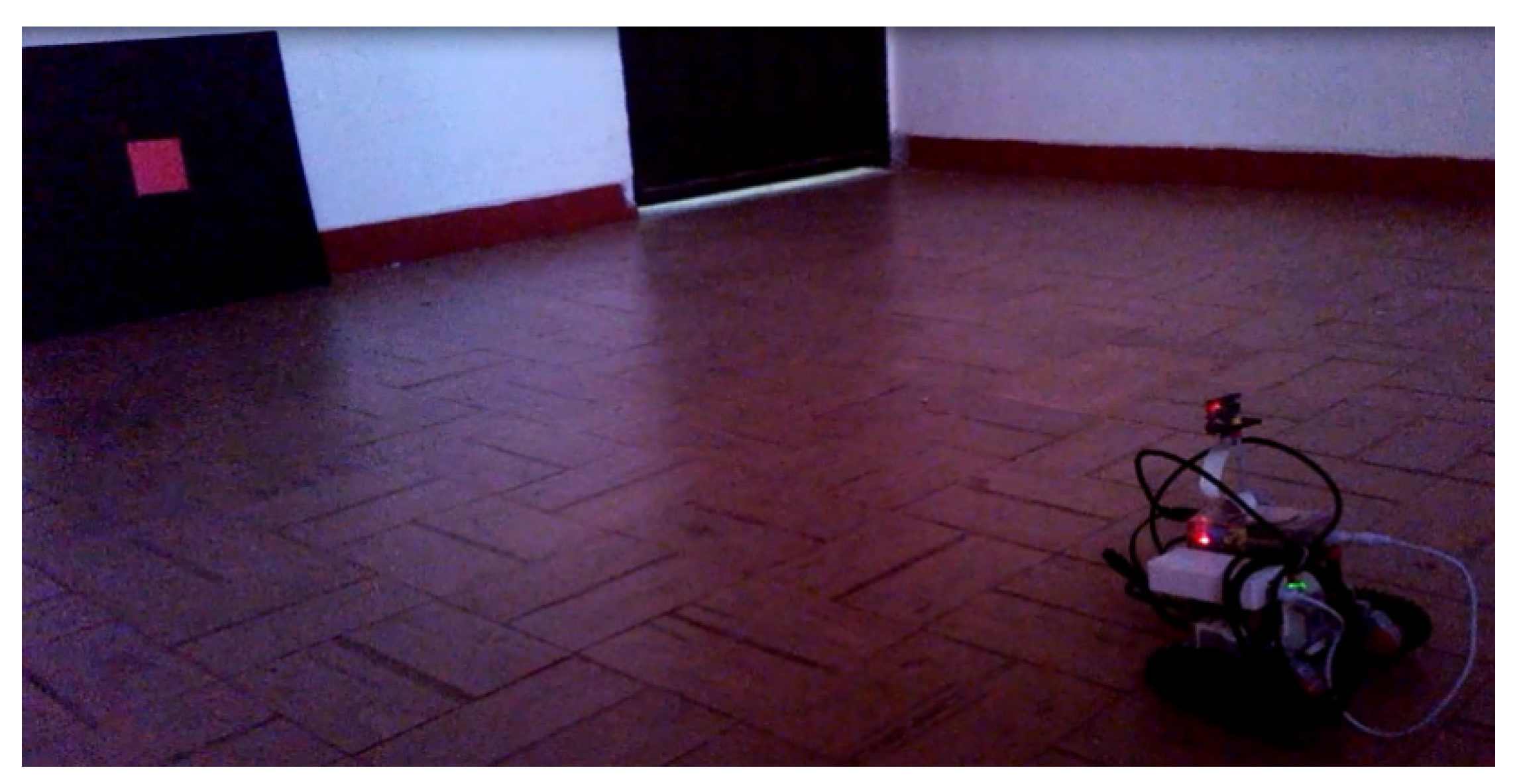
3. Experimental Setup

A communication system between a Raspberry Pi and a mobile interface of a smartphone was integrated on the assembled robot to perform an experimental setup to implement the IBVS control. This proposed 3 DOF robot is operated with an IBVS control scheme based on image detection installed on the operative system of the Raspberry Pi into an SD card, selecting Raspbian mode to support a balanced system. After that, it just remains plugged together with the peripherals: mouse and keyboard, HDMI output for video, and cable. Some software were installed such as OpenCV, SimpleCV libraries, and other libraries required for image processing and control implementation (NumPy, SciPy, and Setuptools), and SSH library for communication with Lego EV3 system [29,30].

3.1. Design of the Communication System between Raspberry Pi and Smartphone

The communication system structure is sketched in Figure 4. First, the configuration to make possible the communication between SSH and LEGO EV3 (Computer Kit LEGO robotics) was defined in order to configure the set of Raspberry Pi to operate as an access point, and in this way, not depend on an external Wi-Fi network. Second, the network Raspberry was created to maintain a fixed IP, assigning this to the smartphone with the Android operating system via the DHCP service.

3.2. Design of Mobile Interface Using a Smartphone

To design and implement the mobile interface (henceforth, mobile app), two sockets to communicate the phone with the Raspberry Pi were used. One of them, to receive data from the phone to the Raspberry Pi, and the other, to send control data. This application was configured in two control modes. First, the automatic mode, where the entire control process is performed by the Raspberry Pi, and second, the manual mode, in which a user operates the robot. Both modes are interchangeable using an eye-shaped button located at the top of the application.

The automatic mode will operate only to monitor the robot, so it was decided to activate a streaming video interface running up as an Android app that communicates to the robot’s camera visualizing and monitoring the surroundings. The app also allows to visualize variables such as the angular speed of each motor of the right engine (${\omega }_{right})$, the left engine (${\omega }_{left}$), and the engine that moves the camera’s platform $({\omega }_{pl}$) (See Figure 5a). In contrast, the manual mode (see Figure 5b), allows access to up to six buttons to manually control the robot. Four of those buttons are used to control stock movements of the robot: forward, backward, right, and left, and the other two buttons are used to control the movement (right and left) of the camera platform. Both modes allow streaming video from the camera. The Mobile app code is found in the Supplementary Materials section.

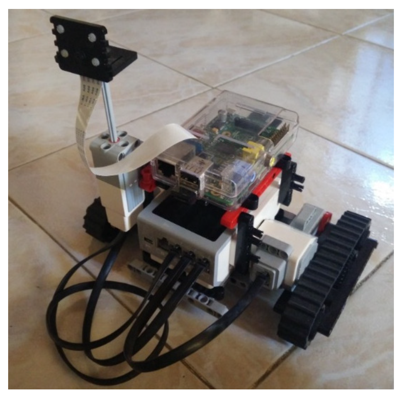
3.3. Assembling the Robot

The robot was assembled using:

• A Kit ™ LEGO Mindstorms robotics for the entire platform, including engines and LEGO EV3 ™ CPU.
• A Single Board Computer Raspberry Pi Model B, with a Pi Camera connected to it via ribbon cable.
• A USB Wi-Fi Dongle TP-LINK TL-WN725N v2.
• An external battery of 5600 mAh.

The final design of the robotic system with the adaptation of the Raspberry Pi and the camera can be seen in Figure 6.

Some simulations were running up to operate this robot using the controllers as shown in the next section.

4. Simulation Results

The concept of Epipolar Geometry is a key topic for simulating visual servo-control systems. This geometry is related to stereoscopic vision. Thus, if one or two cameras are in a 3D scene, there are several geometric relationships between 3D points and their projections on 2D images. These relationships are obtained based on the assumption that the cameras can be approximated by the pinhole model. The Epipolar Geometry Toolbox developed in [31] at the University of Siena was used for the simulation.

Simulations for IBVS, PBVS, and Hybrid controllers are run up using these parameters and the codes reported in [32]:

$$\mathit{X}\mathit{c}=0 cm; \mathit{Y}\mathit{c}=2 cm; \mathit{X}\mathit{p}=5 cm; \mathit{Y}\mathit{p}=5 cm.$$

where $\mathit{X}\mathit{c}$ is the distance from the X-axis from the camera to the platform; $\mathit{Y}\mathit{c}$, the distance from the camera to the platform; $\mathit{X}\mathit{p}$, from the X-axis of the platform to the center of the robot; and $\mathit{Y}\mathit{p}$, from the Y-axis of the platform to the center of the robot.

Figure 7 and Figure 8 show the simulation results of the error of a visual servo control over a robotics system of 3 DOF. Once the previous results were obtained, the next steps were to compute the Jacobian robot, i.e., the 6 × 3 matrix in Equations (3) and (7), and the control law given by (12), (23) considering the real measurements of surrounding by using the parameters mentioned above. Furthermore, the switching rules are followed for the hybrid controller (see Section 2.5).

4.1. Image Error Evolution

Figure 7 shows the simulation of the image error evolution as a time function applying the IBVS (Image Based Visual Servo), PBVS (Position Based Visual Servo),, and the hybrid scheme controllers. For the IBVS control, it can be observed that a minimum error is reached after 1.3 s (see the local minimun), and after there is a negligible increase, similarly, a minimum error is reached after 5 s for PBVS control. Regarding hybrid controller (HBVS), the simulation of image error evolution depends on the time when HBVS is applied. It can be observed that a minimum error is reached after 2.1 s.

The main difference between IBVS and PBVS controls consists of the reference to estimate the error norm. For instance, in IBVS control sensed images, features are extracted and compared using the image plane. In PBVS control image features are also extracted, and this information is used to compute relative position from the object to be compared with the goal relative position. PBVS error is greater than IBVS because they have different units: PBVS error is computed in length units of centimeters, but IBVS error is computed in pixels.

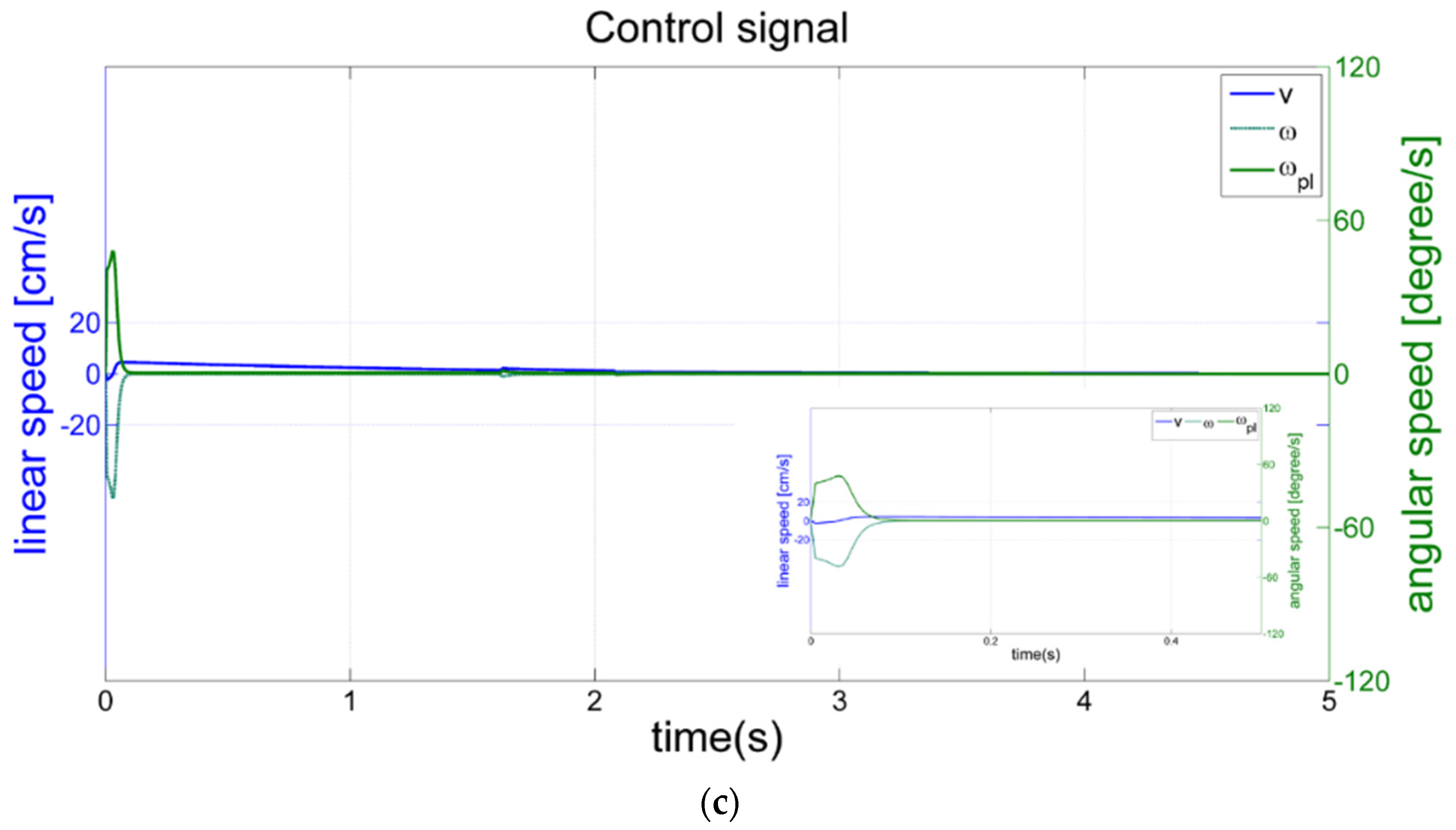
4.2. Control Signal Response

Figure 8 shows the control signals in terms of linear and angular speeds (see Equations (3) and (4)) once one of the IBVS, PBVS, or HBVS algorithms was run up.

The main idea is to use Equation (4) parameters which are the real kinematic of the robot. It can be observed that the control signals respond quickly (see inset Figures) in less than 0.05 s for IBVS, and 0.1 s for PBVS and HBVS.

4.3. Evolution of Image Frame

Figure 9 shows the image evolution of the robot camera (in pixels) in the three cases IBVS, PBVS, and HBVS. For this, a square will be shaped by using the four red points shown in this figure. This will be shown for the IBVS in the next section of the experimental results.

4.4. Initial and Final Pose in 3D

Figure 10 shows the simulation results after applying the IBVS, PBVS, and HBVS controllers, and inverse kinematic (see Equation (4)) to obtain the robot poses.

5. Experimental Results

5.1. Color Image Processing

The fact of how the camera would recognize a square object filled with a specific color was researched in order to characterize the image processed. Several tests were performed with a red square over a black background as shown in Figure 11.

This was the first image successfully processed and recognized. Following this process, red characteristics from the image sensed by the camera were searched. The next step was to invert the image and divide by 16, to get a better contrast for the image by making the algorithm run-up at low resolution. Later, it was necessary to filter to search only those who had a square shape using Algorithm 1 implemented on Python for the Raspberry Pi [33]. As a result of this processing, four points related to the four corners of the square were obtained (See the Supplementary Materials section to obtain the codes for image processing and control algorithm):

Algorithm 1: Feature extraction

Input: Image collected by the camera. Output: set of 4 points coordinates in the image frame, s_i(t). 1 Get the image collected by the camera. 2 Segment the red color. 3 Compare shape (Must be square-like shape). 4 Identify corners. 5 Set coordinates of the points as s_i(t).

5.2. Implementation of the Designed Controller

The control algorithm aims to calculate the control signals for engines, accomplishing the method of the kinematic chain (Jacobian of the robot) and imposing a decreasing behavior to image error. For these calculations, robot Jacobian images as can be seen in Equation (5) represent the optical flow equations that relate to the changes occurring in the image concerning the reference frame of the camera. The Jacobian of the robot, also known as the kinematic chain, is used to apply inverse kinematics to compute the angular speed values that will be applied to the robot engines.

The servo control algorithm (Algorithm 2) running up in Python for Raspberry Pi starts by calculating the Jacobian images (objective and sensed) using Equation (5). It is important to note that this equation describes the behavior of only one point in the image, and then this computing must be realized for all the image features extracted from the camera sensed image, similar to the four points extracted in Section 5.1. Implemented algorithms can be found in the Supplementary Materials section for image processing and control:

Algorithm 2: Control Signal Computing

Input: a set of 4 points coordinates in the image frame, s_i(t). Set of 4 goal points coordinates in the image frame, s_i^*(t). Measurements of θ and θ_pl. Output: Apply control signal to the robot, $\dot{p}$(t). 1 Measure θ and θ_pl. 2 Collect images from the camera. 3 Implement Algorithm 1. 4 Compute image Jacobian Li(s) from Equation (5). 5 Compute the error as is shown in Equation (8). 6 Compute $\dot{p}$(t) from Equation (14). 7 Apply $\dot{p}$(t) to the robot. 8 Go to 1.

Figure 12 shows an external viewpoint during the real implementation of the algorithm of visual servo control for a 3 DOF robotics system. In the Supplementary Materials a video of the operating robot can be found.

6. Conclusions

In this research study, an image-based visual servo for an autonomous mobile robot was modeled and implemented using LEGO EV3 and a Raspberry Pi. This proposed robot operates in two schemes: automatic and manual, with satisfactory performance and recognizing processed image and accurate communication among the three devices: The Raspberry Pi, Lego EV3, and smartphone. This robotic system was designed by running up control IBVS, PBVS, and hybrid algorithms, applied to obtain the inverse kinematic of the robot. The proposed robot is an economic proposal with feature recognition to be used in other settings beyond basic educational programs. It is important to highlight that the assisted video streaming application promotes autonomy using a simple device such as an Android smartphone to easily operate and monitor any objective. For future works, it is proposed to include restrictions on conditions and actuators for better system performance under new parameters, the design of controls considering uncertainties generated by the camera calibration, and the running up of algorithms for feature extractions of more complex images (objectives). These improvements can be implemented by running up algorithms for feature extraction and stereo vision.