
Real-Time Selection System of Dispatching Rules for the Job Shop Scheduling Problem


School of Mechanical and Aerospace Engineering, Jilin University, Changchun 130025, China
*
Author to whom correspondence should be addressed.
Machines 2023, 11(10), 921; https://doi.org/10.3390/machines11100921
Submission received: 23 August 2023
/
Revised: 8 September 2023
/
Accepted: 19 September 2023
/
Published: 22 September 2023
(This article belongs to the Section Industrial Systems)
Abstract
:Personalized market demands make the job shop scheduling problem (JSSP) increasingly complex, and the need for scheduling methods that can solve scheduling strategies quickly and easily has become very urgent. In this study, we utilized the variety and simplicity of dispatching rules (DRs) and constructed a DR real-time selection system with self-feedback characteristics by combining simulation techniques with decision tree algorithms using makespan and machine utilization as scheduling objectives, which are well adapted to the JSSP of different scales. The DR real-time selection system includes a simulation module, a learning module, and an application module. The function of the simulation module is to collect scheduling data in which is embedded a novel mathematical model describing the JSSP; the function of the learning module is to construct a DR assignment model to assign DR combinations to the job shop system, and the function of the application module is to apply the assigned DR combinations. Finally, a series of job shop systems are simulated to compare the DR assignment model with the NSGA-II and PSO algorithms. The aim is to verify the superiority of the DR assignment model and the rationality of the DR real-time selection system.
1. Introduction
Facing market demand for individualized products, companies are trying to improve the flexibility of their manufacturing systems. The production pattern is gradually changing to muti-varieties and small batch [1], which is leading to job shop systems becoming widely available in modern industry. Scheduling, as one of the core modules of a manufacturing system [2,3], assigns jobs to machines in a set of resource constraints and is an important combinatorial optimization problem [4]. The role of job shop scheduling in manufacturing systems has attracted the attention of companies due to the change in production pattern and the importance of scheduling [5]. The job shop scheduling problem (JSSP) belongs to a classical NP-hard problem [6]; its study has important engineering application value and academic significance.
In classical JSSPs, a job set is processed by a machine set of . Any processing sequence of jobs is allowed, the operation order of each job is predefined, and the operations of the jobs may vary from job to job [7]. The general configuration is that the processing time of operation, , of job on machine is known in advance, and there is no pre-emption between jobs.
After decades of research on JSSPs, exact, heuristic, and metaheuristic methods have been developed extensively [8]. The optimal scheduling strategies can be solved by an exact method, such as the simplex algorithm and branch-and-bound algorithm [9,10], but are affected by the computational power and resources, are mostly applied in small-scale and low-complexity production scenarios, and are not suitable for NP-hard problems. Meta-heuristic methods are problem-specific and can solve approximate or even optimal scheduling strategies [11,12]. However, they are prone to fall into local optimal solutions during the problem-solving and their performance is unstable, time-consuming, and poorly migratory, such as genetic algorithms and particle swarm algorithms [13,14]. Heuristic algorithms are efficient, simple, and adaptive [15,16]. They can solve scheduling strategies quickly, are suitable for complex scheduling problems, have much greater solution efficiency than the exact method, and have much shorter solution times than meta-heuristic methods.
Dispatching rule (DR) is a representative heuristic algorithm. The process of solving the scheduling strategy is to set a priority to the jobs according to their parameter values; then, the jobs with higher priority are processed first, with the time taken to solve the scheduling strategy being milliseconds [17]. Due to the advantages of easy implementation and variety, this algorithm can solve scheduling strategies quickly and is often used to solve frequently switching scheduling problems [17,18], such as frequently switching job sets or frequently switching scheduling objectives.
This study utilized the DR to construct a DR real-time selection system with joint simulation, learning, and application modules. One of the most popular scheduling objectives, makespan, was chosen as the primary objective, and machine utilization similar to makespan was the secondary scheduling objective to continuously explore the potential of DR. The contributions of this study mainly include designing a DR real-time selection system with self-feedback characteristics, proposing a DR optimization method for JSSP, constructing a mathematical model to obtain the performance of different DRs, training a DR assignment model to overcome the time-consuming drawback of the simulation technique to search for the optimal DR combination, and comparing the performance of NSGA-II and PSO.
The remainder of this study is organized as follows. Section 2 reviews related work of DR optimization of JSSP. Section 3 proposes a DR real-time selection system with self-feedback characteristics and describes in detail the various modules it contains. Section 4 presents a numerical experiment and training of the DR assignment model using the decision tree algorithm. Section 5 compares the performance of the DR assignment model with NSGA-II and PSO. Section 6 summarizes the study results of this paper and gives an outlook.
2. Literature Review
Examples of literature have been expressing greater interest in DRs, and their research on using DRs in optimizing JSSP mainly includes creating novel DRs, comparing existing DRs, and combining existing DRs.
Creating novel DRs mainly includes two methods: manual and automatic creation [19]. Jayamohan et al. created a series of novel DRs by forming different job parameters [20]. Zhu et al. designed an iterative method based on genetic algorithms to create a series of novel DRs [21]. Methods for automatic DR creation are also given in the literature [22,23]. Manual creation generally requires experts with extensive experience, as designing a good DR is a lengthy trial-and-error process. Although automatically created DRs generally have superior performance to those created manually, the creation process is complex and uninterpretable.
To compare existing DRs is to compare the performance of DRs for different scheduling objectives or job shop systems, and select the best DR. Rohmah et al. [24] selected 14 DRs from the 100 DRs listed by Panwalkar [25] and manually created 30 hybrid DRs, comparing their performance for different scheduling objectives. Marko et al. compared the performance of 26 DRs for different scheduling objective, concluding that DRs exhibited performance close to that of genetic algorithms for some scheduling objectives [17]. Comparing existing DRs has demonstrated that no DR can perform best for different scheduling objectives, and no DR can efficiently schedule job shop systems with different sets of jobs.
Combining existing DRs is one way to optimize the scheduling problem by continuously switching DRs during the production process or selecting multiple DRs at the beginning of scheduling. Zhang et al. correlated DR parameters with scheduling objective semantics and constructed a semantic-based method to optimize the JSSP by DR combination [26]. Metan et al. optimized the JSSP by regularly switching DRs during production with job minimization average delay as the objective [27]. Nasiri et al. proposed a simulation-based multi-response DR combination creation method with the average waiting time of jobs as the scheduling objective [28]. Using DR combination to optimize the JSSP can better combine the advantages of different DRs, but the current study on DR combination to optimize JSSP is scant and mostly focuses on optimizing the JSSP under a single scheduling objective; thus, the potential of DR combination to optimize JSSPs has not been fully exploited.
When optimizing JSSP problems using DRs, a key step is to select the optimal DR or DR combination. Simulation is a powerful tool to test the performance of different scheduling strategies [29]. It can obtain the performance of all alternative DRs or DR combinations in a short time. However, when the number of alternative DRs or DR combinations is very large, it will be limited by its computational power, leading to a time-consuming search for the optimal DR or DR combination, reducing the ability of DRs to optimize JSSPs; even if the computational power is sufficient, it will certainly occupy a large amount of computational resources and increase the cost of DRs to optimize JSSPs.
To overcome the disadvantages of using simulation to search for the best DR or DR combination, which is time-consuming and takes up a large amount of computing resources, scholars have used machine learning, deep learning, and other artificial intelligence algorithms to construct a DR assignment model to assign DRs or a DR combination for the job shop system; each assignment takes very little time and is negligible. Both Metan and Zahmani used decision tree algorithms to construct DR assignment models. Their difference is that Metan assigned DRs during the production process and Zahmani completed the assignment at the beginning of scheduling [27,30]. Azadeh et al. constructed a DR combinatorial assignment model based on an improved neural network algorithm using makespan as the scheduling objective to assign DR-optimized JSSPs to each machine in the job shop system [31]. However, the simulation technique searches for the optimal DR combination considering the mutual influence between DRs, whereas the constructed DR assignment model outputs individual DRs to form a DR combination, which promotes the global optimum by local optimum without considering the mutual influence between DRs. Therefore, the performance of the constructed DR assignment model cannot only be verified at the training level but should continue to be verified at the application level.
By setting novel scheduling objectives and uncovering scheduling problems for production systems, scholars have constructed suitable mathematical models and developed high-performance scheduling algorithms to improve the performance of scheduling strategies and better meet production requirements. Yazdani et al. introduced the sum of the maximum earliness and maximum tardiness criteria as a new scheduling objective, proposed a mixed integer linear programming formulation, and developed an approximate optimization algorithm based on an imperialist competitive algorithm combined with efficient neighborhood search [32]. Zhang et al. proposed a real-time scheduling method based on hierarchical multi-intelligent deep reinforcement learning to solve the dynamic partial no-wait multi-objective flexible job shop scheduling problem with new job insertions and machine failures [33]. Oh et al. considered the variability of the production system when optimizing the scheduling problem and proposed a scheduling method combining independent learners with an implicit quantile network [34].
In summary, scholars have made many contributions to the optimal scheduling problem using DRs, and an increasing number of DR and artificial intelligence algorithms have laid the foundation for continuing to explore the potential of the DR combinatorial optimal scheduling problem. In this study, precisely with the goal of continuing to exploit the potential of DR combinatorial optimization scheduling problems, we designed a self-feedback DR real-time selection system with JSSP as the object of study and makespan and machine utilization as the scheduling objectives, jointly with simulation techniques and artificial intelligence algorithms. This study proposes a method for obtaining job shop scheduling strategies by fusing DR combinations and a mathematical model describing the JSSP. The DR assignment model was trained based on the scheduling data collected during the process of obtaining scheduling strategies, overcoming the disadvantage that the simulation is time-consuming in selecting DR combinations.
3. DR Real-Time Selection System
3.1. DR Real-Time Selection System Proposed
The moment of each DR assignment is defined as a decision point in the scheduling process. The current use of a DR combination to optimize the JSSP is divided into two main methods. One method is to assign DRs by machine at the beginning of scheduling, and to obtain DR combinations at the beginning of scheduling. The other is to divide the scheduling cycle into multiple sub-scheduling cycles as the production process proceeds, and to assign DRs by sub-scheduling cycles; both DR combinations and scheduling strategies are obtained with the production process. Based on these two methods, scholars have optimized static and dynamic JSSPs. Each of the two methods has its own characteristics: one assigns DR to machines and the complexity of forming a DR combination is determined by the number of machines in the production system; the other assigns DR to sub-scheduling cycles and the complexity of forming a DR combination is determined by the number of sub-production cycles. One of the objectives of this study is to combine these methods to form a new DR combination method, where the complexity of forming a DR combination will be determined by the number of machines and sub-scheduling cycles.
As the complexity of the DR combination method proposed in this study increases, the process of selecting the optimal DR combination will be more time-consuming, and constructing a DR assignment model based on artificial intelligence algorithm will be able to overcome this problem well. Therefore, to construct and apply the DR assignment model, based on the data mining process of data collection, model construction, and model application, a DR real-time selection system with self-feedback characteristics was designed. The architecture of the system is shown in Figure 1, where job data are defined as job parameter data that can be obtained directly after obtaining a job task, and scheduling data are defined as data generated in the process of solving a scheduling strategy. The system is supported by a data module and contains a simulation module, a learning module, and an application module, and the functions of each module and the specific relationships between them are described as follows.
The data module contains two database layers, database layer 1 and database layer 2, which store the data necessary for the simulation module and the learning module. Database layer 1 stores job data including job attributes and process data, such as process flow, processing time, etc., which can be obtained directly and is defined as instance data. The instance data in database layer 1 is processed by the simulation module to form scheduling data and stored in database layer 2, which contains rich scheduling knowledge, and the instance data structure in the scheduling data is one job data corresponding to one DR.
The simulation module is responsible for generating the scheduling data, containing the DR combination method and DR set, which is responsible for injecting scheduling knowledge into the instance data to form the scheduling data. Based on the DR combination method defined in advance, a DR is selected from the DR set, defined in advance at each DR assignment moment, all the assigned DRs form a DR combination, and the optimal DR combination is selected from all the alternative DR combinations. The DRs in the DR combination and the job data correspond one by one to form instance data; the combination of all the instance data and the optimal DR form the scheduling data.
The learning module is responsible for extracting the knowledge embedded in the scheduling data in database layer 2, containing data preprocessing methods and decision tree algorithms that are often used to solve scheduling problems [35,36]. The data preprocessing methods include missing value padding, duplicate value deletion, and outlier removal [37]. The missing value padding method embedded in the system is mean padding and the outlier rejection method is the method. The learning module extracts the scheduling data from database layer 2 every time a DR assignment model training command is issued.
The application module is responsible for applying the DR assignment model. When new job data arrive, a request is sent to the learning module at the decision moment, the job data are processed by the data preprocessing method in the learning module, and the processed job data are then input to the DR assignment model to output multiple DRs form a DR combination. Finally, the DR combination is sent to the application module to generate the scheduling strategies, and the newly arrived job data are stored in database layer 1.
Due to the closed-loop process of each module, the scheduling data are constantly updated, and the knowledge coverage of the DR assignment model trained again will be improved, so that the whole system always proceeds in the direction of positive feedback during operation.
The core of the DR real-time selection system lies in the development of a mathematical model and the proposal of a DR combination method. The mathematical model serves as the foundation for the DR combination method, determining the moment of DR assignment. The DR combination method converts instance data into scheduling data using simulation in the simulation module, and assigns DR quickly at the decision-making moment using the DR assignment model in the application module.
3.2. Mathematical Model Construction
The DR assignment method proposed in this study combines assigning DR in units of machines and assigning DR in sub-scheduling cycles. The core of this method is determining the timing of DR assignment. The number of machines being deterministic, the division of sub-scheduling periods plays a crucial role in the performance of the DR assignment method. In this study, a mathematical model describing JSSP is utilized to determine the moment of DR assignment, which is referred to as the scheduling decision point.
A prerequisite for constructing the mathematical model is combining job processing and setup time into job processing time. The assumptions of the mathematical model include the following: no interruptions occur during job processing by the machine, transportation time of the job does not impact the scheduling strategy, each job is only processed once by the machine, jobs are transported to downstream machines immediately after being processed by the machine, each machine only processes one job at a time, and the jobs are independent of each other. The notations of the mathematical model describing the JSSP are shown in Table 1.
The job shop scheduling objective set in this study was to minimize makespan and maximize machine utilization. The objective function is defined as shown in Equations (1) and (2), where Equation (1) indicates minimizing the maximum job completion time and Equation (2) indicates the ratio of actual machine processing time to total running time.
There are machines running simultaneously in the job shop system; each machine may take a different time to complete the current job queue. When a machine completes job queue , another job queue may accumulate on that machine. The size of varies depending on the scheduling strategy in time . The job queue is constantly being completed and accumulated. Therefore, in constructing the mathematical model, two core parameters, and , are introduced. constitutes the set shown in Equation (3), and is solved as shown in Equation (4). If the machine completes one job queue without accumulating another job queue, the machine idles or completes all job tasks.
The scheduling objective makespan can be described as the time when the last job queue is completed, and can be described as the time when machine completes the last queue. Thus, Equation (1) can be transformed into Equation (5), and Equation (2) can be transformed into Equation (6); the whole mathematical model is shown in Equations (5)–(10). The reason for transforming the Equations (1) and (2) into Equations (5) and (6) is that this paper adopts the completion time of the all the jobs in last job queue as the makespan. Additionally, the completion time of each machine for all the jobs in the last job queue is considered as the machine’s completion time.
subject to
Constraint (7) indicates that machine cannot schedule a newly accumulated job queue until it completes the current job queue. Constraint (8) indicates that other machines may have completed multiple job queues while machine completes one job queue. Constraint (9) indicates that the remaining processing time of a job queue is not greater than the processing time of the job queue itself. Constraint (10) indicates the condition that all job queues must be completed.
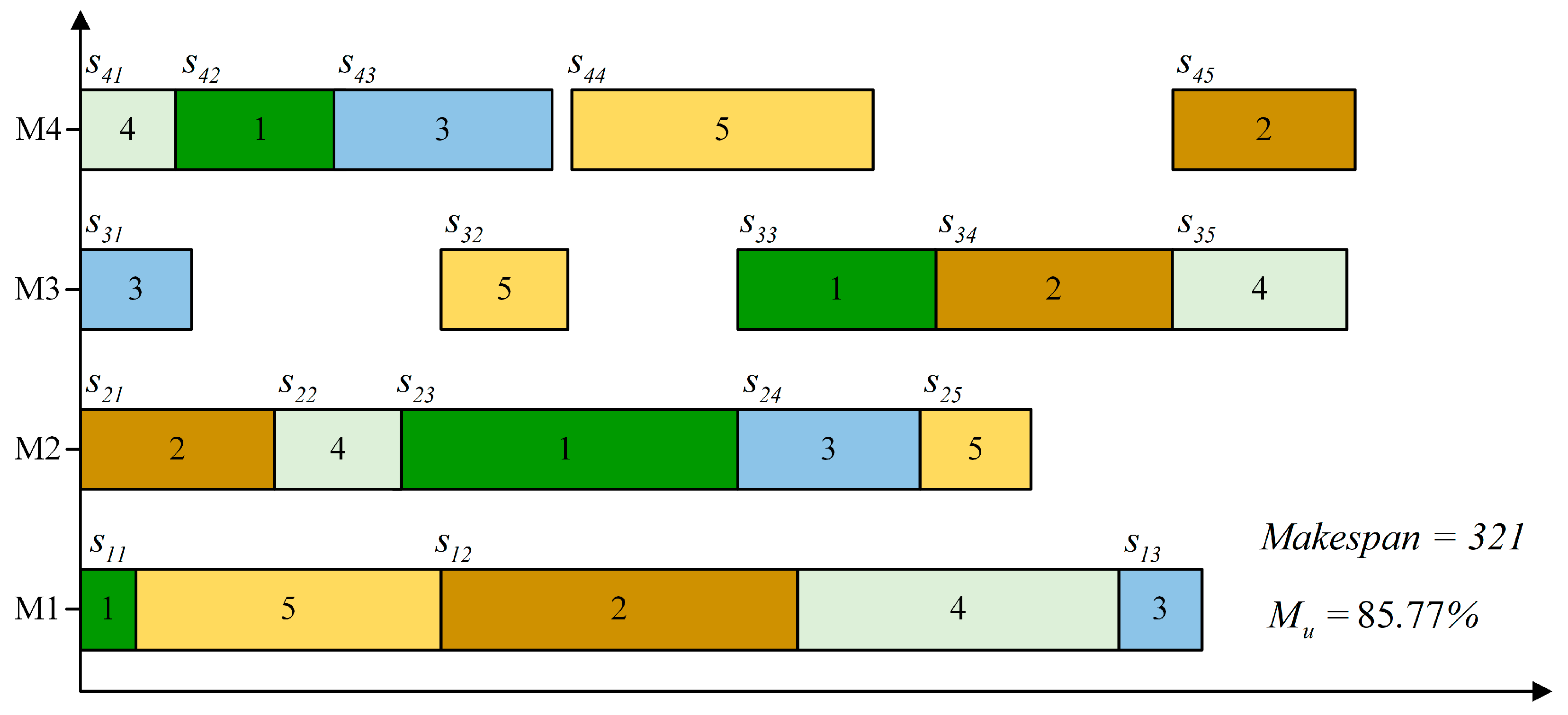
To show the solution process of the above mathematical model more clearly, a 4-machine, 5-job JSSP example is provided as shown in Table 2. The processing sequence (PS) indicates the order in which a job is processed by different machines. For example, in Table 2, the PS of job 1 is 1→4→2→3, indicating that this job goes through machine 1, then machine 4, followed by machine 2, and finally machine 3. At time 0, each machine has a job queue to be processed, and the index of these job queues is 1, denoted as k = 1. At time 0, the time for machine 1 to complete all the jobs in its job queue is 91, the time for machine 2 to complete all the jobs in its job queue rp21 is 90, the time for machine 3 to complete all the jobs in its job queue rp31 is 21, and the time for machine 4 to complete all the jobs in its job queue rp41 is 81. Among them, the job processing sequence of machine 1′s job queue is determined to be 1→5, rp1 = {91, 50, 28, 24}. At time 24, machine 3 completes all the jobs in its job queue, and machine 1 completes job 1 in its job queue, denoted as f1 = 21, rp2 = {67, 26, 4, 43} and k = 2. The time for machine 4 to complete all the jobs in its job queue is rp42 = 43. At time 28, the machine completes all the jobs in the job queue, denoted as f2 = 28, rp3 = {63, 22, 0, 39} and k = 3. The time for machine 3 to complete all the jobs in its job queue is rp33 = 0. Using the scheduling strategy shown in Figure 2 as a guide, continue to iterate according to the above process, and finally obtain f19 = 321, rp19 = {0, 0, 0, 0}. The scheduling policy corresponds to makespan = 321 and machine utilization = 85.77%. Because there are only two jobs in the job queue q12 at the scheduling time s12 in Figure 2, applying processing priority to the jobs in the job queue will affect the scheduling target. When the processing order of the job queue is changed to (4, 2), the makespan is 368 and the machine utilization is 83.19%. Setting processing priority on jobs in the job queue affects productivity.
In this study, the job processing priority in the job queue is determined using the DR assignment method. To reduce the time consumption of DR assignment and job priority determination, the assignment of DR will be triggered when the number of jobs in the job queue is greater than 1 at the time .
4. DR combination Method Proposed
In this study, after the mathematical model is constructed and the scheduling moment is determined, a novel DR assignment method is proposed in combination with the DR assignment model. The scheduling cycle is determined by the machine and the scheduling moment. The machines are divided into sub-scheduling cycles without interfering with each other according to the scheduling moment, one DR is assigned to each sub-scheduling cycle, and multiple DRs are assigned to each machine throughout the scheduling cycle. The assignment moment of a DR is defined as a decision time ; two adjacent decision-making times are defined as a sub-scheduling cycle.
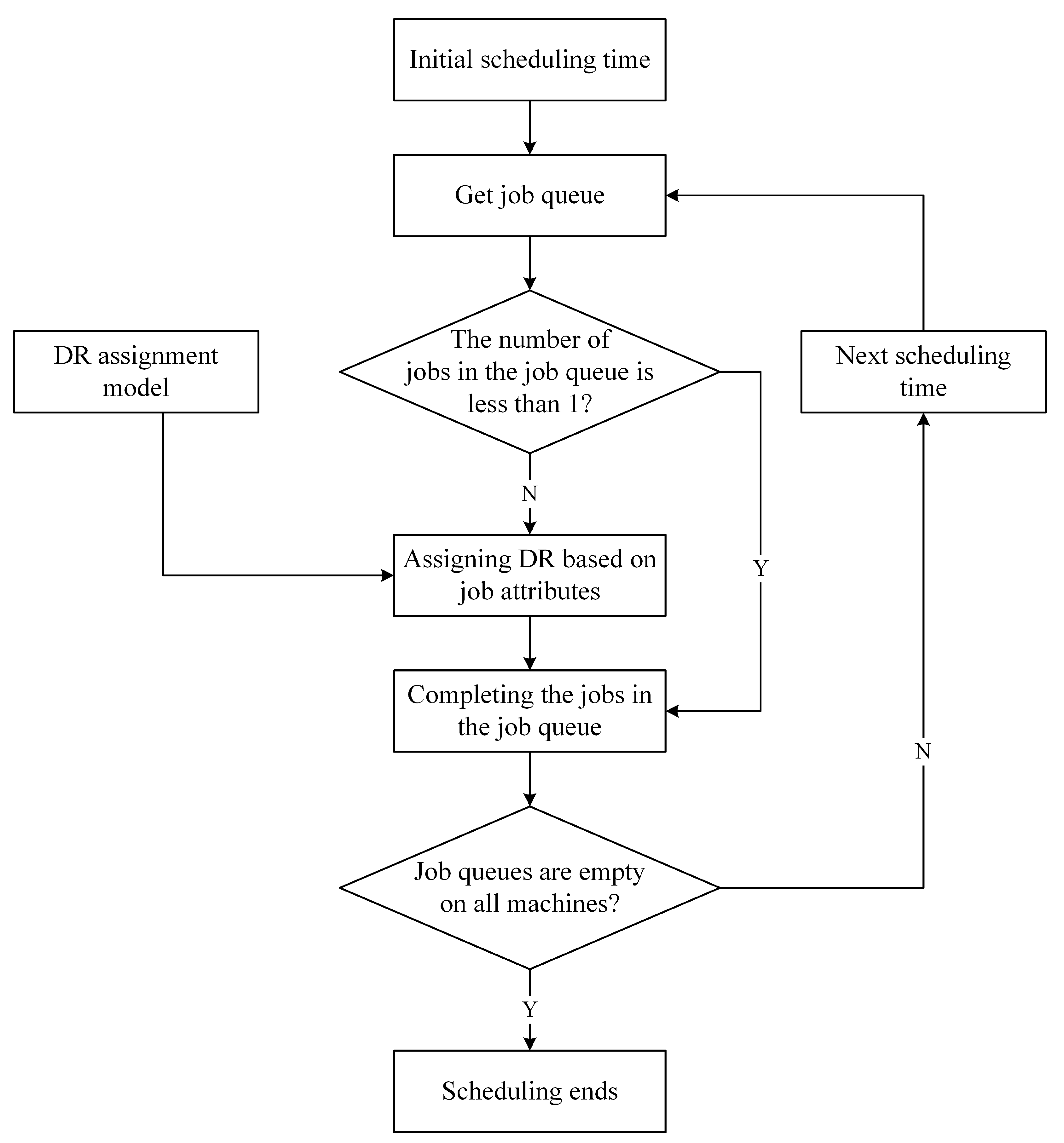
The decision-making process of the DR combination method proposed in this study is showed in Figure 3. Initially, jobs are released to the machines, forming a job queue on each machine. The number of jobs in the queue is then checked. If there is more than 1 job in the queue, a DR is assigned to it. The DR is determined by inputting the job attributes in the queue into the DR assignment model. The assigned DR determines the processing priority of the jobs in the queue. If there is less than 1 job in the queue, no DR is assigned. After completing the jobs in the job queue, the scheduling process ends if the job queues on all machines are empty. Otherwise, the next scheduling moment is entered. Since the scheduling sub-cycle is determined by the scheduling moment, there can be multiple decision points at the same time. The assigned DRs form a DR combination, and the process of assigning the DR combination is defined as the DR combination assignment method. The DR combination method is integrated into the application module.
If the DR assignment process in Figure 3 is converted to selection of DR based on simulation, the optimal DR combination corresponding to the optimal scheduling objective value is chosen after conducting multiple simulations. The production process is then guided by the optimal DR combination to obtain scheduling data. The decision process for the DR combination method is integrated within the simulation module.
5. Experimental Design and DR Assignment Model Construction
The notations referred to in this section and their descriptions are shown in Table 3. The proposed algorithm runs on a laptop with the following capabilities: Intel Core i5-1135G7 [email protected] GHz with 16.0 GB Memory in Windows 10.
5.1. Numerical Experimental Design
In verifying the performance of the proposed DR combination method without considering the perturbations existing in the actual production process, we did not consider machine failures or degradation of the machining capacity. An experimental group and two control groups were designed with the scheduling objective of optimizing the makespan and machine utilization of the production system. The experimental group was the DR assignment model to optimize the performance of JSSP, and the two experimental groups were PSO and NSGA-II to optimize the performance of JSSP. To compare the performance between the above experimental and control groups, the whole experimental process is described in Figure 4, including two parts of model construction and performance comparison; the specific process is presented subsequently.
The process of model construction is as follows: first, the job shop production systems were generated, and the tasks in the job shop under the set scheduling objective were completed as a JSSP; then, the job data in the JSSP were extracted and a DR library was created to generate scheduling data after simulation; finally, the data were mined in the scheduling knowledge to train a DR assignment model using the decision tree algorithm. The process of performance comparison is as follows: first, a new set of JSSPs was generated according to the method of generating JSSPs in the model construction process; then, scheduling strategies were generated using the DR assignment model, PSO, and NSGA-II and the obtained scheduling objective values were solved; finally, we compared the performance of the DR assignment model and PSO, and the performance of the DR assignment model and NSGA-II. The parameter setting of JSSP, the construction of DR set, and the training of DR assignment model should be implemented in the experiment.
5.2. DR Set Construction
This study constructed a DR set with reference to the DR created by Kaban et al. [24], including static DR and dynamic DR. The parameter value of static DR is the static attribute of the job, and the parameter value of dynamic DR is the dynamic attribute of the job. The static attribute value of the job will not change over time, including the processing time (PT), the time required by machine to process job , and its value of ; the processing sequence (PS) is the total operand required to complete job in the production system, and its value is . Total processing time (TPT) is the total operating time required to complete job in the production system; its value is . The dynamic attribute values of the job will change over time, including waiting time (WT), the time that job waits on machine queue for scheduling decision, with its value is ; total work remaining (TWR) is the total operation time remaining required to complete job in the production system, with a value of .
The process of creating a DR is shown in Equation (11), where represents the new attribute value of the job, and and represent two different attribute values of the job. The DR sets the priority of the job to be processed according to the value of the job. The smaller the value, the higher the priority. In Table 4, the ✓ symbol is the combination of two job parameters into one dispatching rule parameter; the symbol × is vice versa. Ten hybrid DRs were created: a static DR is PT × PS, PT × TPT, and PT × PS; a dynamic DR is PT × WT, PT × TWR, PS × WT, PS × TWR, TPT × WT, TPT × TWR, and WT × TWR.
5.3. JSSP Parameter Setting
To verify the superiority of the DR combination method in this paper, many JSSP examples were selected; this section describes a method for generating JSSPs based on the processing characteristics of the job shop. Only two categories of production elements, machines and materials, were considered in the job shop production system when generating JSSPs. Each machine has different functions; for products, each job has variability in the processing time and order of being processed on different machines. The time that a job takes to be processed on a machine obeys the geometric distribution of . The difference between and determines the variance of jobs, and the larger the difference, the greater the variance between jobs; if , operation is not executed; the number of jobs contained in a JSSP obeys the integer distribution of .
In this study, we set and , selected JSSPs of 3, 4, 5, and 6 machine scales, and generated 10,000 instance data values for each scale to construct the DR assignment model in order to eliminate the chance when the proposed method optimized the scheduling problem.
5.4. Simulation Process Design
For the DR combination method proposed in this paper, the number of simulations required to search for the optimal DR combination by simulation is shown in Equation (12), where cannot be obtained at the early stage of production scheduling, which is unknown and cannot be found at the early stage of production scheduling.
The decision moment is generated with the production, which cannot be obtained at the early stage of production scheduling; therefore, is unknown at the early stage of production scheduling, and cannot be solved. Thus, the DR combination method proposed in this paper cannot search for the optimal DR combination.
To address the problem of not being able to exhaust all DR combinations, and thus search for the optimal DR combinations, as shown Figure 5, this study proposes a method for determining the number of simulations, setting the number of simulations, , in stages, and taking the DR combinations corresponding to the optimal objective value in all stages as the optimal dispatching rule combinations when no better scheduling objective value is searched for in three consecutive stages than in the previous one. The specific implementation process is shown in Figure 3: the optimal scheduling objective value is after the first stage simulation search; the optimal scheduling objective value is after the second stage simulation search; if is inferior to , the third stage simulation search for the optimal scheduling objective value is . If is inferior to , the fourth and fifth stages of the search are conducted in turn, and the cumulative objective values of the three stages, , , and , are found to be inferior to the scheduling objective value searched in the second stage; then the DR combination corresponding to is taken as the optimal DR combination and is the optimal scheduling objective value. Conversely, the search continues until there are three consecutive stages in which no better scheduling objective value is found compared with the previous stage. Here, during each simulation, as the production process reaches a decision moment, a DR is randomly selected from the DR set as the DR to be called at that decision moment.
5.5. DR Assignment Model Construction
After obtaining scheduling data with scheduling knowledge through simulation technology, feature selection and creation are performed first: feature selection selects the job processing time (PT), the job processing sequence (PS), the total processing time (TPT) of the job in the manufacturing system, and the job process flow (PP) as job attribute data, where the process flow PP data are processed by ordinal coding to transform them into numerical data; new job attribute data are created, including the job waiting time (WT), the remaining job processing time (TWR), and parameters of the hybrid DR which are shown in Table 4.
After initiating the DR real-time selection system, the training flow of the DR assignment model is shown in Figure 6. When the job set is sent to the job shop, the job data are collected, and the scheduling data are first processed according to the predefined feature selection and data preprocessing methods; then, the DR assignment request is sent to the learning module. If there is a DR assignment model in the learning module, the processed scheduling data are input into the model to output the DR. If there is no DR assignment model in the learning module, the scheduling data are extracted from the database, the scheduling data are processed according to the predefined feature selection and data preprocessing rules, and then a decision tree algorithm is selected to construct a DR assignment model. The feature selection and data preprocessing methods described above are the same.
The DR assignment model is trained by dividing the collected scheduling data into training and prediction datasets in the ratio of 7:3, and the DR assignment model is trained by searching the optimal parameters using the fivefold grid search method. The performance of the DR assignment models constructed under JSSP with different machine sizes, using accuracy as the evaluation index, is shown in Table 5. The correct prediction rate of the DR assignment model constructed under JSSP with a three-machine-scale is 88.67%; the correct prediction rate of the DR assignment model constructed under JSSP with a four-machine-scale is 88.7%; the correct prediction rate of the DR assignment model constructed under JSSP with a five-machine-scale is 78.61%; and the correct prediction rate of the DR assignment model constructed under JSSP with a six-machine-scale is 86.22%. Overall, the prediction performance is acceptable.
6. Performance Analysis
After the DR assignment model was constructed, the model was applied in the application module. However, when solving the scheduling strategies by DR, it is necessary to correspond to multiple job data in order to be effective. Therefore, at the decision time, a DR is assigned to each job in the queue of jobs to be processed at the machine, and the DR is determined by the “majority rule” principle for the assigned DR.
Referring to the method of generating JSSPs in Section 5.3 to generate 1000 JSSPs, the DR assignment model constructed in this paper was compared with the existing NSGA-II and PSO algorithms. NSGA-II and PSO are widely used metaheuristic algorithms for solving JSSPs. Previous research on JSSPs has primarily focused on improving the performance of NSGA-II or PSO algorithms [38,39], solving specific JSSPs using NSGA-II or PSO algorithms [40,41], and using NSGA-II or PSO algorithms as benchmarks to evaluate proposed scheduling methods [42,43]. The purpose of this paper is to further enhance machine utilization after achieving the optimal makespan. The optimization of the two scheduling objectives follows the above sequence. By utilizing the PSO algorithm, multiple scheduling strategies with the same makespan can be generated during the search for a feasible solution. From these strategies, the scheduling strategy that maximizes machine utilization can be selected for further optimization. The comparative box plots of makespan and machine utilization scheduling objectives for different JSSP scales are shown in Figure 7, Figure 8, Figure 9 and Figure 10. Although the NSGA-II is superior to the DR assignment model in terms of the degree of optimization, it is less stable, and the DR assignment model outperforms both other two algorithms from an overall perspective. Using the mean value as the indicator, the advanced performance of the DR assignment model is detailed in Table 6.
On the makespan scheduling objective, for the three-machine-scale JSSP, the DR assignment model is 8.83% optimized compared with NSGA-II and 23.21% optimized compared with PSO; for the four-machine-scale JSSP, the DR assignment model is 8.28% optimized compared with NSGA-II and 18.77% optimized compared with PSO; for the five-machine-scale JSSP, the DR assignment model is 7.6% optimized compared with NSGA-II and 18.04% optimized compared with PSO; for the six-machine-scale JSSP, the DR assignment model is 9.24% optimized compared with NSGA-II and 17.02% optimized compared with PSO. Under the machine utilization scheduling objective, for the three-machine-scale JSSP, the DR assignment model is 3.56% optimized compared with NSGA-II and 10.78% optimized compared with PSO; for the four-machine-scale JSSP, the DR assignment model is 1.83% optimized compared with NSGA-II and 10.15% optimized compared with PSO; for the five-machine-scale JSSP, the DR assignment model is 2.04% optimized compared with NSGA-II and 11.29% optimized compared with PSO; for the six-machine-scale JSSP, the DR assignment model is 2.09% optimized compared with NSGA-II and 11.08% optimized compared with PSO.
In this study the concept of designing a DR real-time selection system to optimize JSSPs is to divide the production scheduling cycle into multiple sub-scheduling cycles, and to obtain the optimal scheduling strategy for local sub-scheduling cycles to promote the optimal global scheduling strategy; the process of obtaining scheduling data based on simulation technology is static. The process of using artificial intelligence algorithms to mine knowledge from scheduling data and construct DR assignment models, which assigns DR to sub-scheduling cycles and thus obtains scheduling strategies, is dynamic. The above idea transforms the static generation of global scheduling strategies into the dynamic generation of sub-scheduling strategies, which can be used to optimize dynamic scheduling problems, such as applications to perturbation problems caused by job release, machine degradation, etc.
The scheduling strategy’s time for DR to solve can be demonstrated in milliseconds, as referenced in [17]. This paper’s scheduling method assigns DRs to job queues, and the number of DR combinations are huge. To expedite the assignment of DRs with superior performance to each job queue, we employ machine learning to train the DR assignment model. The time advantage of pre-training the DR assignment model is evident in the process of assigning DRs in units of machines, as referenced in [27,30]. Consequently, combining the advantages of DR and DR assignment models can lead to reduced CPU solution times. We compared the solution time of different scheduling methods for JSSPs, as shown in Table 7, where m*n is used to represent the JSSP scale. Therefore, the CPU solution time advantage of the proposed method is proved.
The experiments conducted in this study demonstrate that the proposed scheduling method can obtain more effective scheduling strategies within a shorter time. The scheduling method involves dividing the sub-scheduling cycles and assigning DRs to each sub-scheduling cycle using a pre-trained DR assignment model. Subsequently, each DR generates a locally optimal scheduling strategy, which contributes to the overall optimal global scheduling strategy. The DR assignment model, trained using data from the globally optimal scheduling strategy, retains the performance advantage of using simulation to search for the optimal scheduling strategy and reduces the waiting time between jobs. Moreover, due to the clear time relationship between sub-scheduling cycles, this process exhibits dynamic characteristics. By transforming the static scheduling strategy assignment process into a dynamic scheduling strategy assignment process, the proposed scheduling method shows potential in optimizing dynamic scheduling problems, such as those arising from the release of new jobs and machine degradation.
7. Conclusions
In this study, a DR real-time selection system was designed by combining simulation, a decision tree algorithm, and DRs. With makespan and machine utilization as the scheduling objectives, a novel DR combination method was embedded in the simulation module and a mathematical model was constructed; a DR assignment model was trained using the decision tree algorithm to achieve the real-time and efficient generation of local scheduling strategies, which, in turn, promotes optimal global scheduling strategies. To verify the performance of the DR assignment model, which is the core of the system, a numerical experiment was set up to compare the NSGA-II algorithm with an average optimization of 8.49% for makespan and an average optimization of 2.38% for machine utilization at three-, four-, five-, and six-machine JSSP scales, and the PSO algorithm with an average optimization of 19.26% for makespan and an average optimization of 10.825%.
Although the research in this paper has achieved some results, there are still many shortcomings, and future research should focus on the following aspects: finding or creating advanced DR to enrich the DR library, proposing more suitable data mining algorithms to improve the generalization ability of the model and mitigate the adverse effects of prediction errors on the objectives values, and taking into account the perturbations that may be encountered inside and outside the workshop to make the application scenarios of the method proposed in this paper more realistic. In addition, the process of assigning DRs by the DR assignment model is similar to the training process of reinforcement learning. Further research can be conducted by combining the mathematical model in this paper with reinforcement learning.
Author Contributions
Conceptualization, A.Z.; data curation, A.Z.; formal analysis, A.Z.; funding acquisition, P.L.; investigation, P.L.; methodology, A.Z.; project administration, L.H.; software, L.H.; resources, H.L.; supervision, Z.X.; validation, Y.L.; visualization, H.L.; writing—original draft, A.Z.; writing—review and editing, A.Z. All authors have read and agreed to the published version of the manuscript.
Funding
This work was supported by Jilin Scientific and Technological Development Program (Grant no. 20210201037GX) and Jilin Major Science and Technology Program (Grant no. 20210301037GX).
Data Availability Statement
The authors confirm that the data supporting the findings of this study are available within the article.
Conflicts of Interest
We would like to declare no conflict of interest exits in the submission of this manuscript, and the manuscript is approved by all authors for publication. We also would like to declare on behalf of my co-authors that the work described is original research that has not been published previously, and not under consideration for publication elsewhere, in whole or in part. All the authors listed have approved the manuscript that is enclosed.
References
- Leng, J.; Jiang, P.; Liu, C.; Wang, C. Contextual self-organizing of manufacturing process for mass individualization: A cyber-physical-social system approach. Enterp. Inf. Syst. 2018, 14, 1124–1149. [Google Scholar] [CrossRef]
- Li, X.; Guo, X.; Tang, H.; Wu, R.; Wang, L.; Pang, S.; Liu, Z.; Xu, W.; Li, X. Survey of integrated flexible job shop scheduling problems. Comput. Ind. Eng. 2022, 174, 108786. [Google Scholar] [CrossRef]
- Kress, D.; Müller, D.; Nossack, J. A worker constrained flexible job shop scheduling problem with sequence-dependent setup times. OR Spectr. 2018, 41, 179–217. [Google Scholar] [CrossRef]
- Zhang, M.; Tao, F.; Nee, A.Y.C. Digital Twin Enhanced Dynamic Job-Shop Scheduling. J. Manuf. Syst. 2021, 58, 146–156. [Google Scholar] [CrossRef]
- Strusevich, V.A. Complexity and approximation of open shop scheduling to minimize the makespan: A review of models and approaches. Comput. Oper. Res. 2022, 144, 105732. [Google Scholar] [CrossRef]
- Chaouch, I.; Driss, O.B.; Ghedira, K. A novel dynamic assignment rule for the distributed job shop scheduling problem using a hybrid ant-based algorithm. Appl. Intell. 2018, 49, 1903–1924. [Google Scholar] [CrossRef]
- Taillard, E. Benchmarks for basic scheduling problems. Eur. J. Oper. Res. 1993, 64, 278–285. [Google Scholar] [CrossRef]
- Zhang, L.; Hu, Y.; Wang, C.; Tang, Q.; Li, X. Effective dispatching rules mining based on near-optimal schedules in intelligent job shop environment. J. Manuf. Syst. 2022, 63, 424–438. [Google Scholar] [CrossRef]
- Zhang, G.; Xing, K.; Zhang, G.; He, Z. Memetic Algorithm With Meta-Lamarckian Learning and Simplex Search for Distributed Flexible Assembly Permutation Flowshop Scheduling Problem. IEEE Access 2020, 8, 96115–96128. [Google Scholar] [CrossRef]
- Braune, R. Packing-based branch-and-bound for discrete malleable task scheduling. J. Sched. 2022, 25, 675–704. [Google Scholar] [CrossRef]
- Zhu, H.; Tao, S.; Gui, Y.; Cai, Q. Research on an Adaptive Real-Time Scheduling Method of Dynamic Job-Shop Based on Reinforcement Learning. Machines 2022, 10, 1078. [Google Scholar] [CrossRef]
- Türkyılmaz, A.; Şenvar, Ö.; Ünal, İ.; Bulkan, S. A research survey: Heuristic approaches for solving multi objective flexible job shop problems. J. Intell. Manuf. 2020, 31, 1949–1983. [Google Scholar] [CrossRef]
- Amirteimoori, A.; Mahdavi, I.; Solimanpur, M.; Ali, S.S.; Tirkolaee, E.B. A parallel hybrid PSO-GA algorithm for the flexible flow-shop scheduling with transportation. Comput. Ind. Eng. 2022, 173, 108672. [Google Scholar] [CrossRef]
- Wang, Z. Optimal Scheduling of Flow Shop Based on Genetic Algorithm. J. Adv. Manuf. Syst. 2021, 21, 111–123. [Google Scholar] [CrossRef]
- Zarrouk, R.; Bennour, I.E.; Jemai, A. A two-level particle swarm optimization algorithm for the flexible job shop scheduling problem. Swarm Intell. 2019, 13, 145–168. [Google Scholar] [CrossRef]
- Ɖurasević, M.; Jakobović, D. Creating dispatching rules by simple ensemble combination. J. Heuristics 2019, 25, 959–1013. [Google Scholar] [CrossRef]
- Ðurasević, M.; Jakobović, D. A survey of dispatching rules for the dynamic unrelated machines environment. Expert Syst. Appl. 2018, 113, 555–569. [Google Scholar] [CrossRef]
- Sels, V.; Gheysen, N.; Vanhoucke, M. A comparison of priority rules for the job shop scheduling problem under different flow time- and tardiness-related objective functions. Int. J. Prod. Res. 2012, 50, 4255–4270. [Google Scholar] [CrossRef]
- Branke, J.; Nguyen, S.; Pickardt, C.W.; Zhang, M. Automated Design of Production Scheduling Heuristics: A Review. IEEE Trans. Evol. Comput. 2016, 20, 110–124. [Google Scholar] [CrossRef]
- Jayamohan, M.S.; Rajendran, C. New dispatching rules for shop scheduling: A step forward. Int. J. Prod. Res. 2010, 38, 563–586. [Google Scholar] [CrossRef]
- Zhu, X.; Guo, X.; Wang, W.; Wu, J. A Genetic Programming-Based Iterative Approach for the Integrated Process Planning and Scheduling Problem. IEEE Trans. Autom. Sci. Eng. 2022, 19, 2566–2580. [Google Scholar] [CrossRef]
- Planinic, L.; Backovic, H.; Durasevic, M.; Jakobovic, D. A Comparative Study of Dispatching Rule Representations in Evolutionary Algorithms for the Dynamic Unrelated Machines Environment. IEEE Access 2022, 10, 22886–22901. [Google Scholar] [CrossRef]
- Teymourifar, A.; Ozturk, G.; Ozturk, Z.K.; Bahadir, O. Extracting New Dispatching Rules for Multi-objective Dynamic Flexible Job Shop Scheduling with Limited Buffer Spaces. Cogn. Comput. 2018, 12, 195–205. [Google Scholar] [CrossRef]
- Kaban, A.K.; Othman, Z.; Rohmah, D.S. Comparison of dispatching rules in job-shop scheduling problem using simulation: A case study. Int. J. Simul. Model. 2012, 11, 129–140. [Google Scholar] [CrossRef] [PubMed]
- Panwalkar, S.S.; Iskander, W. A Survey of Scheduling Rules. Oper. Res. 1977, 25, 45–61. [Google Scholar] [CrossRef]
- Zhang, H.; Roy, U. A semantics-based dispatching rule selection approach for job shop scheduling. J. Intell. Manuf. 2018, 30, 2759–2779. [Google Scholar] [CrossRef]
- Metan, G.; Sabuncuoglu, I.; Pierreval, H. Real time selection of scheduling rules and knowledge extraction via dynamically controlled data mining. Int. J. Prod. Res. 2010, 48, 6909–6938. [Google Scholar] [CrossRef]
- Nasiri, M.M.; Yazdanparast, R.; Jolai, F. A simulation optimisation approach for real-time scheduling in an open shop environment using a composite dispatching rule. Int. J. Comput. Integr. Manuf. 2017, 30, 1239–1252. [Google Scholar] [CrossRef]
- Zuting, K.R.; Mohapatra, P.; Daultani, Y.; Tiwari, M.K. A synchronized strategy to minimize vehicle dispatching time: A real example of steel industry. Adv. Manuf. 2014, 2, 333–343. [Google Scholar] [CrossRef]
- Zahmani, M.H.; Atmani, B. A Data Mining Based Dispatching Rules Selection System for the Job Shop Scheduling Problem. J. Adv. Manuf. Syst. 2019, 18, 35–56. [Google Scholar] [CrossRef]
- Azadeh, A.; Negahban, A.; Moghaddam, M. A hybrid computer simulation-artificial neural network algorithm for optimisation of dispatching rule selection in stochastic job shop scheduling problems. Int. J. Prod. Res. 2012, 50, 551–566. [Google Scholar] [CrossRef]
- Yazdani, M.; Aleti, A.; Khalili, S.M.; Jolai, F. Optimizing the sum of maximum earliness and tardiness of the job shop scheduling problem. Comput. Ind. Eng. 2017, 107, 12–24. [Google Scholar] [CrossRef]
- Zhang, Y.; Zhu, H.; Tang, D.; Zhou, T.; Gui, Y. Dynamic job shop scheduling based on deep reinforcement learning for multi-agent manufacturing systems. Robot. Comput.-Integr. Manuf. 2022, 78, 102412. [Google Scholar] [CrossRef]
- Oh, S.H.; Cho, Y.I.; Woo, J.H. Distributional reinforcement learning with the independent learners for flexible job shop scheduling problem with high variability. J. Comput. Des. Eng. 2022, 9, 1157–1174. [Google Scholar] [CrossRef]
- Jun, S.; Lee, S. Learning dispatching rules for single machine scheduling with dynamic arrivals based on decision trees and feature construction. Int. J. Prod. Res. 2020, 59, 2838–2856. [Google Scholar] [CrossRef]
- Habib Zahmani, M.; Atmani, B. Multiple dispatching rules allocation in real time using data mining, genetic algorithms, and simulation. J. Sched. 2020, 24, 175–196. [Google Scholar] [CrossRef]
- Alexandropoulos, S.-A.N.; Kotsiantis, S.B.; Vrahatis, M.N. Data preprocessing in predictive data mining. Knowl. Eng. Rev. 2019, 34, 1–33. [Google Scholar] [CrossRef]
- Huo, D.; Xiao, X.; Pan, Y.J. Multi-objective energy-saving job shop scheduling based on improved NSGA-II. Int. J. Simul. Model. 2020, 19, 494–504. [Google Scholar] [CrossRef]
- Zhou, Z.; Xu, L.Y.; Ling, X.F.; Zhang, B.K. Digital-twin-based job shop multi-objective scheduling model and strategy. Int. J. Comput. Integr. Manuf. 2023, 16, 1–21. [Google Scholar] [CrossRef]
- Amelian, S.S.; Sajadi, S.M.; Navabakhsh, M.; Esmaelian, M. Multi-objective optimization for stochastic failure-prone job shop scheduling problem via hybrid of NSGA-II and simulation method. Expert Syst. 2022, 39, e12455. [Google Scholar] [CrossRef]
- Sha, D.Y.; Lin, H.H. A multi-objective PSO for job-shop scheduling problems. Expert Syst. Appl. 2010, 37, 1065–1070. [Google Scholar] [CrossRef]
- Mahmud, S.; Chakrabortty, R.K.; Abbasi, A.; Ryan, M.J. Switching strategy-based hybrid evolutionary algorithms for job shop scheduling problems. J. Intell. Manuf. 2022, 33, 1939–1966. [Google Scholar] [CrossRef]
- Li, J.X.; Wen, X.N. Construction and simulation of multi-objective rescheduling model based on PSO. Int. J. Simul. Model. 2020, 19, 323–333. [Google Scholar] [CrossRef]
Figure 1.
DR real-time selection system architecture.

Figure 2.
Gantt chart of the instance for JSSP.

Figure 3.
DR combination method decision process.

Figure 4.
Flow of the comparison experiment.

Figure 5.
DR combination method simulation number determination process.

Figure 6.
DR assignment model construction process.

Figure 7.
Performance comparison under the 3-machine-scale JSSP.

Figure 8.
Performance comparison under the 4-machine-scale JSSP.

Figure 9.
Performance comparison under the 5-machine-scale JSSP.

Figure 10.
Performance comparison under the 6-machine-scale JSSP.


Table 1.
Notations description of mathematical model.
| Notations | Descriptions |
|---|---|
| The index of machine, | |
| The index of job, | |
| The index of job queue, | |
| The job queue of the machine | |
| The completion time of machine | |
| The completion time of job queue | |
| The time of the last job queue in the last machine (makespan) | |
| Process time of the job on the machine | |
| Process time of the queue on the machine | |
| The remaining processing time for job queue , if machine is idling, | |
| The set composed of at the time of machine complete job queue | |
| The time of the job queue is completed, | |
| The time when machine completed the last job queue | |
| The difference in index during the completion of job queue | |
| The time of the job queue is scheduled on machine , |
Table 2.
Job shop production system with four machines and five jobs.
| Job | Machine 1 | Machine 2 | Machine 3 | Machine 4 | PS |
|---|---|---|---|---|---|
| 1 | 14 | 87 | 50 | 43 | 1→4→2→3 |
| 2 | 90 | 50 | 60 | 46 | 2→1→3→4 |
| 3 | 21 | 46 | 28 | 55 | 3→4→2→1 |
| 4 | 81 | 28 | 44 | 24 | 4→2→1→3 |
| 5 | 77 | 28 | 32 | 76 | 1→3→4→2 |
Table 3.
Notations description of experimental process.
| Notations | Descriptions |
|---|---|
| The processing time of the job on the machine | |
| PT | The processing time parameter of the job, its value |
| The processing sequence of job | |
| PS | The processing sequence parameter of the job, its value is |
| The total processing time of job | |
| TPT | The total processing time parameter of the job, its value is . |
| The time that job waits on machine queue for scheduling decision | |
| WT | The total processing time parameter of the job, its value is |
| The total operation time remaining required to complete job | |
| TWR | The total processing time parameter of the job, its value is . |
| The first parameter value of job on the machine | |
| The second parameter value of job on the machine | |
| The mixed parameter values of job on the machine | |
| , | The upper and lower bounds of in the job shop system |
| , | The upper and lower bounds of the number of jobs in the job shop system |
| The total number of decision moments in the whole scheduling cycle | |
| The number of DRs in the DR set | |
| The number of theoretical simulations to search for the optimal DR combination | |
| The actual number of simulations to search for DR combinations | |
| The optimal scheduling results obtained after simulations in the rth stage |
Table 4.
The hybrid DR created by Kaban et al. [24].
Table 4.
The hybrid DR created by Kaban et al. [24].
| Parameter | PT | PS | TPT | WT | TWR |
|---|---|---|---|---|---|
| PT | ✘ | ✓ | ✓ | ✓ | ✓ |
| PS | ✘ | ✘ | ✓ | ✓ | ✓ |
| TPT | ✘ | ✘ | ✘ | ✓ | ✓ |
| WT | ✘ | ✘ | ✘ | ✘ | ✓ |
| TWR | ✘ | ✘ | ✘ | ✘ | ✘ |
Table 5.
Predictive performance of the DR assignment model.
| Machine Scales | 3 | 4 | 5 | 6 |
|---|---|---|---|---|
| Accuracy (%) | 78.61 | 88.67 | 88.7 | 86.22 |
Table 6.
DR assignment model optimization compared with the NSGA-II method.
| Scheduling Objective | 3-Machine | 4-Machine | 5-Machine | 6-Machine |
|---|---|---|---|---|
| Makespan | 8.83% | 8.28% | 7.6% | 9.24% |
| Machine utilization | 3.56% | 1.83% | 2.04% | 2.09% |
Table 7.
CPU solution time with comparison algorithms.
| JSSP | 20 × 3 | 60 × 3 | 100 × 3 | 20 × 4 | 60 × 4 | 100 × 4 | 20 × 5 | 60 × 5 | 100 × 5 | 20 × 6 | 60 × 6 | 100 × 6 |
|---|---|---|---|---|---|---|---|---|---|---|---|---|
| DR-M | 2.3 | 7.4 | 9.8 | 3.1 | 9.3 | 13.9 | 4.2 | 14.2 | 18.8 | 4.7 | 15.3 | 20.1 |
| NSGA-II | 7.6 | 20.6 | 32.1 | 9.1 | 24.5 | 35.8 | 12.8 | 39.3 | 49.2 | 16.2 | 43.2 | 66.2 |
| PSO | 8.1 | 22.3 | 34.5 | 9.7 | 25.6 | 37.1 | 14.1 | 42.1 | 51.3 | 17.1 | 45.6 | 68.5 |
Disclaimer/Publisher’s Note: The statements, opinions and data contained in all publications are solely those of the individual author(s) and contributor(s) and not of MDPI and/or the editor(s). MDPI and/or the editor(s) disclaim responsibility for any injury to people or property resulting from any ideas, methods, instructions or products referred to in the content. |
© 2023 by the authors. Licensee MDPI, Basel, Switzerland. This article is an open access article distributed under the terms and conditions of the Creative Commons Attribution (CC BY) license (https://creativecommons.org/licenses/by/4.0/).
Share and Cite
MDPI and ACS Style
Zhao, A.; Liu, P.; Li, Y.; Xie, Z.; Hu, L.; Li, H. Real-Time Selection System of Dispatching Rules for the Job Shop Scheduling Problem. Machines 2023, 11, 921. https://doi.org/10.3390/machines11100921
AMA Style
Zhao A, Liu P, Li Y, Xie Z, Hu L, Li H. Real-Time Selection System of Dispatching Rules for the Job Shop Scheduling Problem. Machines. 2023; 11(10):921. https://doi.org/10.3390/machines11100921
Chicago/Turabian StyleZhao, Anran, Peng Liu, Yunfeng Li, Zheyu Xie, Longhao Hu, and Haoyuan Li. 2023. "Real-Time Selection System of Dispatching Rules for the Job Shop Scheduling Problem" Machines 11, no. 10: 921. https://doi.org/10.3390/machines11100921
Note that from the first issue of 2016, this journal uses article numbers instead of page numbers. See further details here.