
Urban Platooning Combined with Dynamic Traffic Lights


Department of Control for Transportation and Vehicle Systems, Faculty of Transportation Engineering and Vehicle Engineering, Budapest University of Technology and Economics, Műegyetem Rkp. 3, 1111 Budapest, Hungary
*
Author to whom correspondence should be addressed.
Machines 2023, 11(9), 920; https://doi.org/10.3390/machines11090920
Submission received: 29 August 2023
/
Revised: 17 September 2023
/
Accepted: 20 September 2023
/
Published: 21 September 2023
(This article belongs to the Special Issue Artificial Intelligence for Automatic Control of Vehicles)
Abstract
:Platooning is generally known as a control method for driving a group of connected and automated vehicles in motorway context. Nevertheless, platoon control might also work on urban roads. One possible strategy to increase overall road traffic performance and to reduce congestion in urban traffic networks is to combine platooning with traffic signal control at intersections. The traffic flow can be maximized with coordinated scheduling of traffic signals together with platooning activities, resulting in decreased travel times and fuel consumption. This paper investigates several aspects of this combined control, such as the procedures for coordination and communication between platooning vehicles and traffic signals. Efficient algorithms are suggested to optimize platoon formation and dissolution at junctions and to change traffic signal phases depending on platoon arrival and departure times. The proposed solutions have been tested and verified with SUMO, a high-fidelity microscopic traffic simulator.
1. Introduction
The term platooning [1] is used to describe the practice of forming a number of vehicles into a tight, coordinated formation. Platooning formation has arisen as a form of efficient vehicle convoy control [2] that has the potential to solve critical traffic issues, such as congestion, traffic safety hazards, or air pollution problem. The practice of forming groups of cars to travel in tight formation improves traffic flow by allowing more cars on the road at once without causing additional congestion, thanks to the reduced but controlled spacing between vehicles and guaranteed constant speeds. A further vital advantage is that it is environmentally sustainable. When cars drive in a platoon, they are able to maximize fuel economy and to reduce greenhouse gas emissions, two factors that are crucial to the development of sustainable transportation systems [3]. Moreover, with the recent developments of the automated vehicle functions [4,5], platooning is getting closer to everyday application, possibly in the near future.
Technologically, platooning systems take advantage of classical control theory or machine learning, as well as vehicle-to-vehicle (V2V) communication to mimic the efficiency of natural phenomena like bird flocks. On the other hand, when it comes to regulating and directing traffic flow in urban contexts, smart intersections shall become game-changers. Smart intersections represent a subset of Intelligent Transport Systems (ITS) intending to improve the effectiveness and safety of traffic flow in the vicinity of road crossings. Smart junctions require the use of recent developments in sensing, processing, and communicating data to realize traffic-responsive intersection management. In order to reduce traffic jams, accident risks, and environmental effects, numerous smart intersection methods have been investigated [6], and the potential has also been revealed when intersection control is realized with the consideration of automated vehicle technologies [7,8].
While platooning has been a hot topic of automotive developments for decades, vehicle convoy control in an urban context combined with traffic lights is still an open problem with limited solutions. Ref. [9] provides signal timing optimization in connected transportation networks by considering platoons; however, no direct platooning control is applied in their framework. There is also much research on control determining optimal speed profiles for individual cars in the vicinity of signalized intersections, e.g., [10]. However, these approaches do not provide a solution to platoon control. A pioneering work on this topic is the paper of [11] (“Traffic Signal Control by Leveraging Cooperative Adaptive Cruise Control (CACC) Vehicle Platooning Capabilities”). This study focuses on a new cooperative traffic signal algorithm for enhancing the CACC vehicle string operation but still has limitations. Firstly, it does not investigate a specific platooning algorithm; instead, the paper only utilizes the characteristics of this technology. Regarding the traffic light control logic, it only deals with the green time duration of the given signal phase (increasing or decreasing) according to the volume of traffic. Furthermore, the signal control algorithm cannot go back to the previous cycle, even if a sudden increase in traffic volume happens, i.e., it has to complete the whole current cycle. In all, throughout our literature research, we have identified several research gaps in the existing literature. Our study aims to address the revealed gaps. We propose novel scientific contributions that advance the fields of traffic signal control and CACC vehicle platooning.
As a summary of the state of the art in intelligent intersection control together with platooning, we can conclude that the existing solutions are rather focused on traffic light control based on the actual platooning data and do not intend to influence the platoon control, i.e., a form of effective combined control has not been established yet. The main scientific contributions of our work are itemized below, highlighting the main innovations.
- Compared with the state of the art in traffic light control methods, a PID (Proportional–Integral–Derivative) controller-based platooning model was applied combined with traffic light system (TLS) control.
- The proposed TLS logic is not limited to keeping the same Signal Phase and Timing (SPaT) [12] cycle order as in previous solutions. Calculations give the needed time for the current active lane with the actual vehicle, which is managed to initiate vehicle-to-infrastructure (V2I) communication, and the TLS will trace that vehicle until it successfully passes through the intersection (before it is allowed to open the TLS controlling communication again).
- The proposed dynamic algorithm focuses on the approaching vehicles sending signals to the traffic light (via V2I communication). Priority calculation is based on the speed and location of vehicles, i.e., faster vehicles can cross the intersection more efficiently.
2. The State of the Art of Platooning Operation and Smart Intersections
In this part, a brief literature review is provided to review the state-of-the-art solutions of platoon control.
2.1. Theoretical Framework of Platooning
Communication protocols and the dissemination of information play crucial roles in the technological architecture of platooning. V2V communication is a crucial part of the platooning ecosystem sharing information about their current location, speed, as well as acceleration/deceleration. Dedicated Short Range Communication (DSRC), which is largely utilized to provide collision prevention applications, cellular vehicle-to-everything (C-V2X) technology, and upcoming 5G networks all support this kind of data transmission in real time. “According to estimates from the U.S. Department of Transportation DSRC can prevent up to 82% of all crashes in the country” [13], making it one of the principal applications of V2V communication. Another use of V2V is present in CACC systems, where cars form platoons and modify their speeds based on the information they obtain from the vehicles ahead of them [14]. When cars move in convoy, the front vehicle shields the rear vehicles from the wind, lowering the drag they experience, i.e., the cars behind can greatly benefit from this phenomenon, which is known as slipstreaming or drafting [15].
When it comes to platooning, sensor systems play crucial roles in collecting data. Multiple types of vehicle sensors, including radar, LIDAR (Light Detection and Ranging), ultrasonic, radar, optical cameras, infrared, and vision sensors, collaborate to provide a detailed, real-time image of the world around the vehicle [16]. These parts are essential for the safety and effectiveness of platooning because they identify possible obstructions, track vehicle attributes, and monitor the actions of neighboring road users in real time [17]. Sensor fusion [18] is also essential for overcoming the difficult challenge of moving object recognition and tracking in autonomous vehicles.
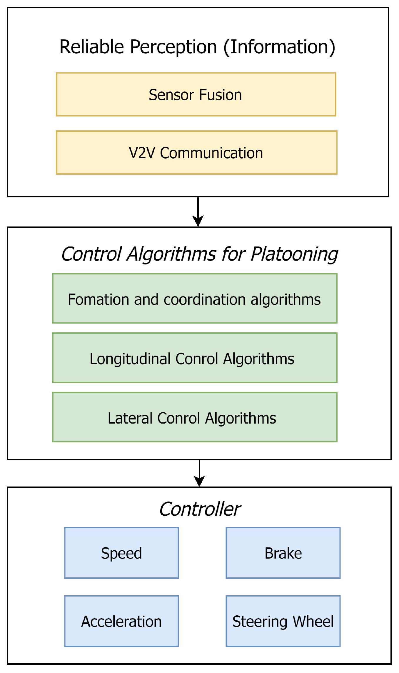
Control systems [17] serve as the platooning operation’s central nervous system by processing information from the vehicle sensors and adjusting the vehicle behavior accordingly. CACC and similar technologies are also embedded in these control systems [19]. Important processes including acceleration, deceleration, steering, and braking are controlled by their interpretation of the vast amounts of sensory data. They do this by constantly updating the cars’ speed and direction based on real-time data, allowing for the most efficient formation possible while also improving fuel economy and traffic flow. The general flowchart of the platooning architecture is illustrated in Figure 1. Primarily, it comprises three key stages. The initial stage involves information perception, as previously discussed, followed by the application of various platooning algorithms in the subsequent phases. Formation and coordination algorithms, or merging and leaving algorithms are the foundation of a platooning system, ensuring that vehicles within a platoon behave predictably and cooperatively. These algorithms strike a balance between efficient traffic flow and road safety, enabling the safe entry and exit of vehicles onto the highway while reacting appropriately to changes in speed or direction initiated by the lead vehicle. The longitudinal control algorithm, represented later by the PID controller, serves as CACC, and governs the acceleration and deceleration of platoon vehicles, maintaining consistent distances and smoothing traffic flow. Equally crucial are lateral control algorithms, responsible for keeping vehicles within their lanes, enhancing platoon stability, and reducing lane departure incidents. These algorithms play a significant role in maintaining platoon cohesion, ensuring driver safety, and optimizing traffic control. And lastly, the controller can take an action.
2.2. Smart Intersections
Platoons of cars can improve their efficiency and lessen traffic congestion by communicating with smart traffic lights. Some platoon movements that may be used in conjunction with an intelligent traffic signal system are as follows: before the platoon reaches the junction, the light is preemptively changed to green by sending a signal to the traffic light system. This means the platoon can get to the junction just as the light turns green, saving time otherwise spent waiting. Multiple options for improving platoon efficiency and overall traffic flow at traffic light intersections are provided by the intelligent traffic light system. Green wave (or coordinated control of TLS) coordinates the timing and phases of traffic lights along a route such that a platoon traveling at a certain speed always arrives at green lights. This shortens the time it takes between platoon stops and increases productivity. Platoons are more productive on the road because of this prioritizing, which reduces wait times and guarantees a smooth passage for them. Platooning vehicles may benefit from real-time traffic information and make more educated judgments about speed, formation, and route. Platoons can improve their road safety and efficiency by planning ahead for things like traffic signal changes and anticipated congestion. In all, intelligent TLS techniques and characteristics play a crucial role in improving traffic flow at crossings, decreasing congestion, and optimizing platoon travel. The technology enhances efficiency, cuts down on delays, and promotes a safer and more convenient trip for all road users by permitting seamless coordination between platoons and traffic signals.
To function, smart intersections must rely on one-way or rather two-way communication networks, such as V2I, I2V, or infrastructure-to-infrastructure (I2I) communication. With the use of V2I communication, traffic lights can update drivers on traffic conditions in real time, allowing drivers to modify their speeds to ease congestion, save money on gas, and cut down on pollution. Optimizing traffic flow and facilitating informed decision-making are both facilitated by I2I communication between traffic control devices and central traffic management systems. Real-time traffic management enables V2I and I2V connections, in which the information is shared among cars and traffic management systems. With V2V communication, automobiles may coordinate and travel more safely by exchanging data about their current conditions. Advanced communication technologies like Dedicated Short Range Communication (DSRC), cellular networks, and satellite communications or upcoming 5G networks are only some of the technologies used by these networks [20,21]. Having access to SPaT provides a number of benefits. Green Light Optimal Speed Advisory (GLOSA) [7] or Green Light Optimal Dwell Time Advisory (GLODTA) [22] are two driver assistance systems that may be implemented and integrated with this upgrade to the regular Transit Signal Priority [23].
3. Methodology for Combined Platooning and Dynamic Traffic Light Control
In this part, the detailed methodology for combined control of platooning and TLS is provided.
3.1. Test Bed for Algorithm Development and Testing: SUMO and TraCI
Throughout our research, a validated simulation test bed was applied. SUMO (Simulation of Urban Mobility) [24] is an open-source, microscopic traffic simulation software, which also provides a flexible extension for customizable interfacing with the simulation, called TraCI (Traffic Control Interface). SUMO and TraCI enable realistic, simulation-based analysis. In a SUMO simulation, each car is considered as individual agent with the so-called car-following (microscopic) driving behaviour. SUMO together with TraCI allows users to set the vehicle parameters, the road network, and the simulation during run time. These software tools provide an efficient method for simulating and analyzing a wide range of potential road conditions that platooning cars may experience. Our investigation of SUMO and TraCI’s fundamental capabilities will shed light on how these tools might be used to model platooning systems in simulation. We intend to provide a holistic view of how various simulation settings aid in our knowledge of and progress toward platooning technology through our investigation.
3.2. Platooning Realization Using PID Control
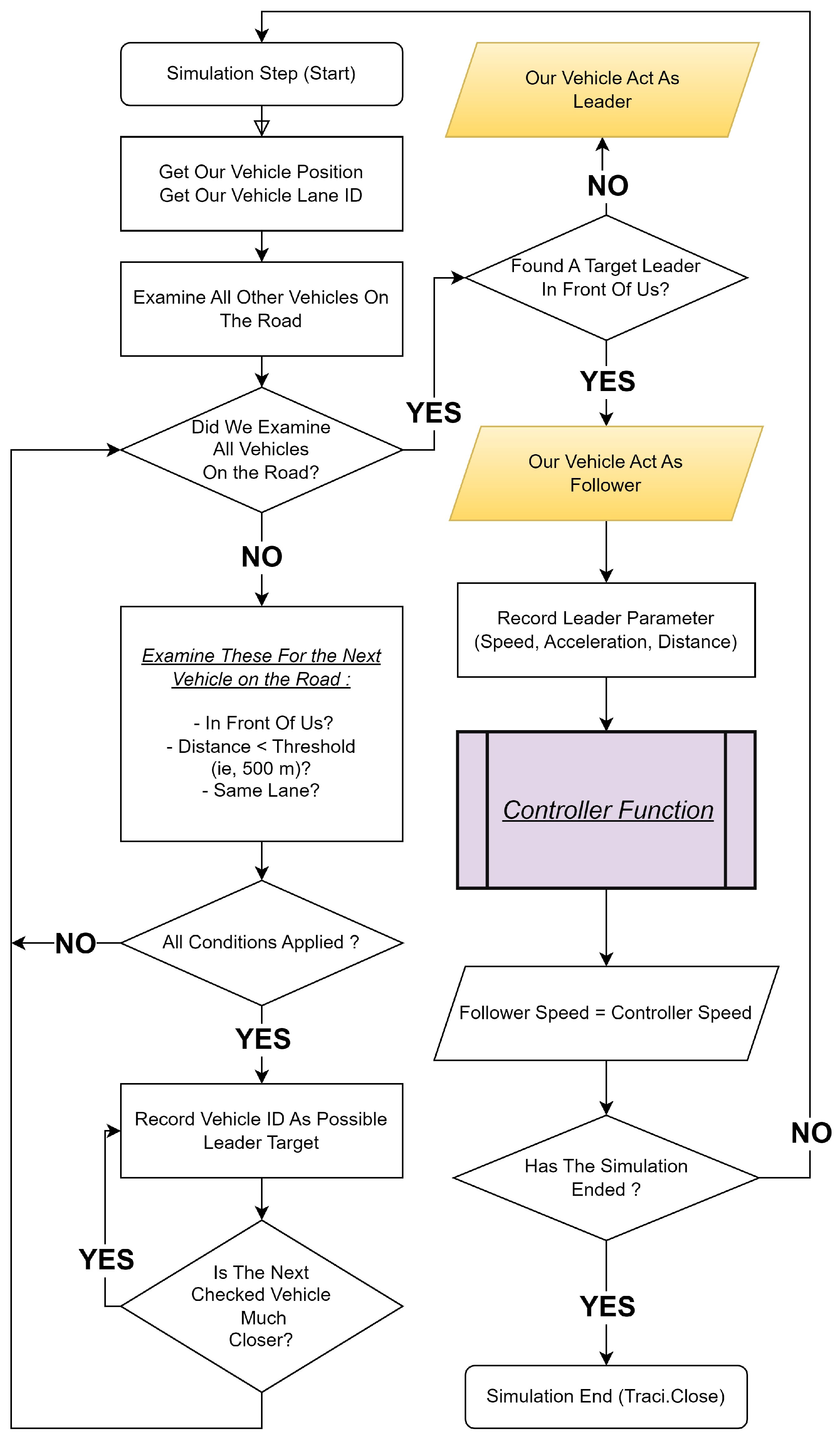
We provide a summary of the platooning realization with a PID controller using SUMO TraCI programming. In a platoon, a number of vehicles move in close proximity to each other in a synchronized fashion, which can be regulated by a properly designed PID controller. In order to perform smooth dynamics, vehicles within the platoon must coordinate their speed, location, and distance compared with the others. In real-world realization, detecting obstacles, keeping appropriate distances, or enabling coordinated actions are all supported by the use of cutting-edge sensors and automated systems. The PID controller is designed by assuming these technologies as available and generally following the workflow shown in Figure 2. This figure illustrates the formation and management of platooning on the road. The process begins with a vehicle scanning the road for a suitable leader based on specific criteria, including a matching destination and an acceptable gap distance. When these criteria align, the vehicle transitions into a follower role, gradually closing the gap to the leader. Subsequently, a PID controller assumes control to maintain a consistent distance between the follower and the leader. Alternatively, if the vehicle cannot identify a suitable leader, it can take on the role of a leader, guiding other followers in the platoon.
3.2.1. Target Vehicle Selection
In platooning, target vehicle selection refers to the process by which a platooning system identifies and selects a certain vehicle to operate as the platoon’s leader or target. This decision is critical for getting and keeping a platoon of cars on the road. The chosen target vehicle usually contains particular characteristics or satisfies certain requirements that qualify it to lead the platoon. These criteria may include elements such as the destination being the same as that of the follower vehicles, the vehicle’s speed, its ability to maintain a consistent pace, and its compatibility with the platoon’s objectives. Target vehicle selection is an important part of platooning technology since it affects the platoon’s overall performance and cooperation on the road. The algorithm shall select a target vehicle for each of the followers by applying certain conditions. First, the logic checks if the leader and follower are in the same lane. Then, the distance between them will be calculated. In the controlled case, the software will instruct the follower to move at a predetermined speed.
3.2.2. The Applied PID Controller
In control engineering, the Proportional–Integral–Derivative (PID) controller is a well-known and effective method for influencing the system behavior in a feedback control system. In our platooning approach, the PID controller considers the target vehicle’s speed and acceleration, as well as the distance between the leader and the follower, to determine the appropriate reference velocity for the followers at all times. If the controller detects a target vehicle, the follower’s speed is determined with the controller function (see Equation (1)). In the SUMO simulation test bed, vehicle data (including locations, lanes, speeds, and distances) were all retrieved via specific TraCI methods. Based on the retrieved data, the implemented PID controller provides the controlled speed function as follows:
The control input function, provided by Equation (1), requires four parameters and three coefficients that have been carefully selected to ensure the best platooning performance and to maintain a smooth formation, i.e., larger values may result in automatic emergency braking, AEB, while smaller values lead toward less efficient controller algorithm, where always represents the difference between a given parameter at the leader and that of the follower. denotes the follower car’s current velocity. represents the difference in vehicles’ speeds, which is weighted by the proportional term ( was chosen to provide a reasonable response to changes in ). is the actual headway distance (difference between the front bumpers of the leader and follower), while H is the target headway distance to be achieved. We use headway and not clearance in this equation, since we are dealing with TraCI language programming, which only measures the headway but not clearance. For example, if we want to keep the clearance at 6 m, then we should add the vehicle length to it, so we can obtain the desired total headway H; now, we are able to subtract it from . In this way, the clearance was kept at 6m. The integrator part of the PID controller multiplies the difference between the target and the current distance, i.e., the term modifies the control input by eliminating the steady-state error ( was chosen to minimize steady-state errors and to maintain system stability). is the acceleration difference between the leader and follower vehicles. The derivative term of the PID controller weights so that the control input is also influenced by the acceleration difference of the vehicles. On the other hand, intends to stabilize the system response ( was chosen to reduce overshoot and improve transient response).
The function ensures a practical constraint so that the speed adjustments never go above a specified threshold (maximum 0.8 m/s).
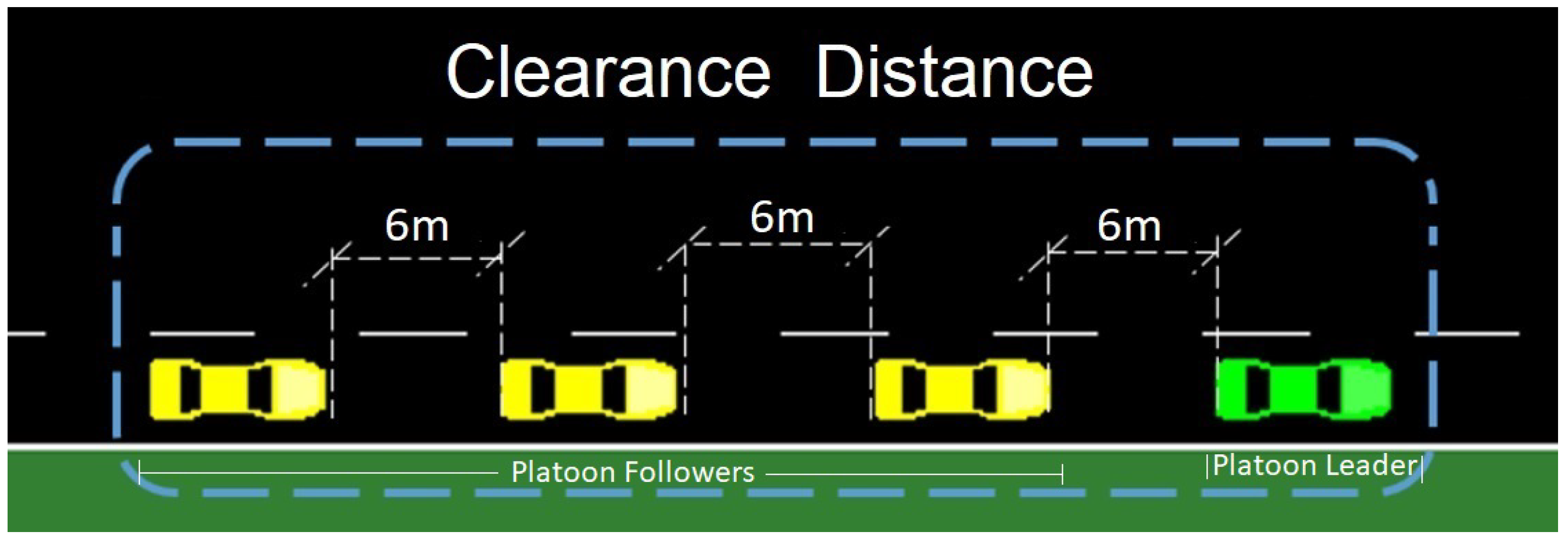
3.2.3. Choosing an Appropriate Clearance Parameter
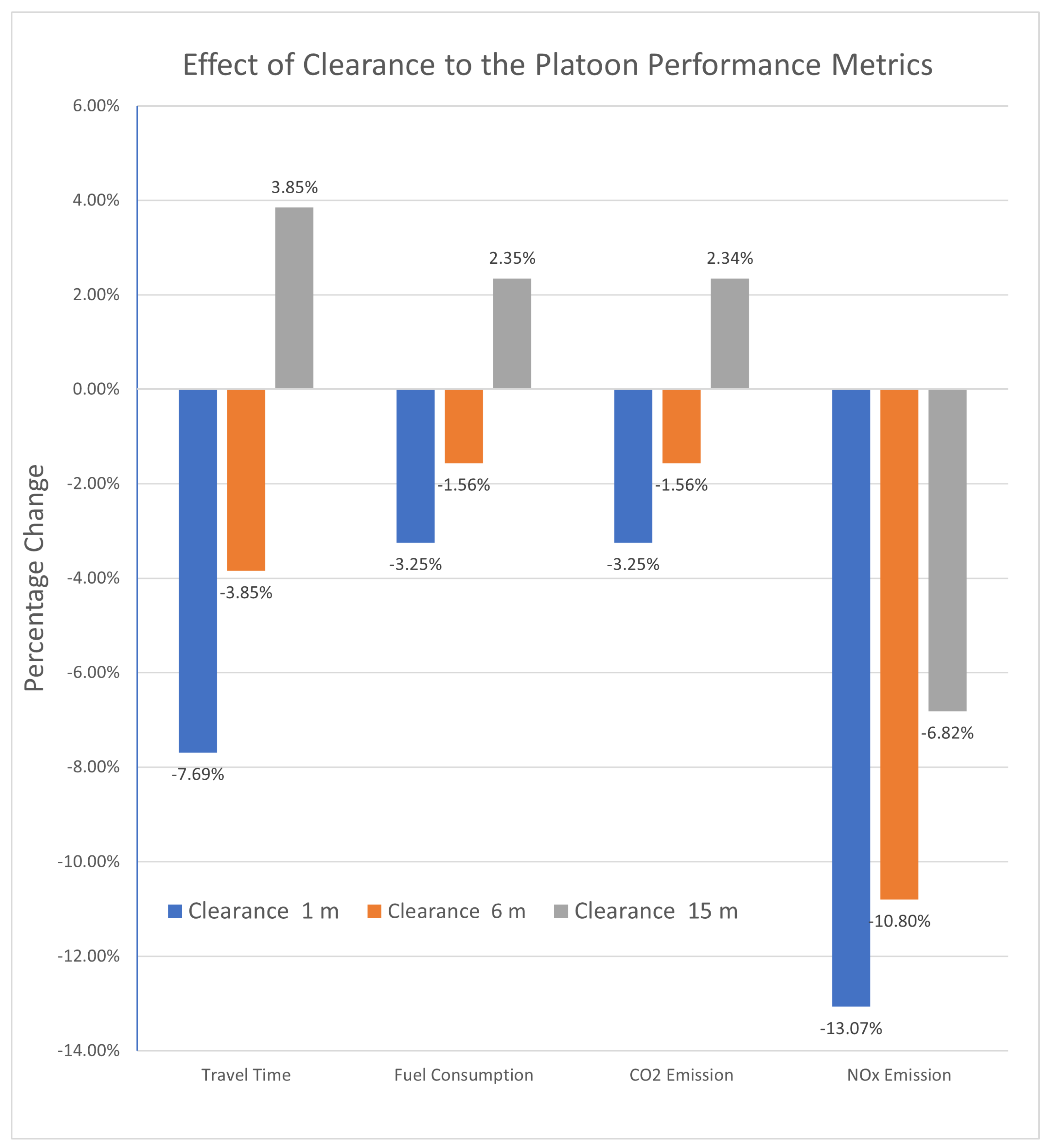
The desired safety level, traffic circumstances, and vehicle characteristics and the intended use of the platooning system all play important roles in defining the optimal clearance value for platoon formation (Figure 3). This diagram illustrates a standard platoon on the road, with the leader designated in green and the followers indicated in yellow. When setting up a platoon, the clearance parameter determines the desired clearance distance or time gap (if it is measured as time) between the leader’s tail and the follower’s front in the platoon. The clearance must ensure the safe dynamics of the platoon even in the case of sudden maneuvers, i.e., rapid braking or steering. The optimal clearance is to be adaptable depending on the traffic volume and average velocity on the given road link. For instance, bigger clearance is needed in the case of heavy traffic together with higher speed. Furthermore, the specific features of the cars (acceleration/deceleration capability or reaction time) must be considered in the platoon. Besides the vehicle-specific characteristics, the general objective of the platooning also influences the applied clearance, e.g., if traffic flow maximization is the top priority, smaller headway is preferred so that as many cars as possible may leverage the given road capacity. Furthermore, guidelines or regulations for the minimum allowable headway parameter may be provided by local legislation or industry standards in the future. Figure 4 is a result of testing platooning performance where it experiences different clearance values at 1 m, 6 m, or 15 m. So, at each clearance value, we have conducted two experiments, a controlled scenario (platooned) and non-controlled one (traditional human driving). We measured the performance metrics (travel time, fuel consumption, and CO2 and NOX emissions) in each case and then calculated the percentage change as platooning was applied. Equation (2) was used to calculate the relative change.
What this study suggests is that applying different clearance values will result in different performance outcomes. Overall, clearance distance is a very crucial part of platooning, and choosing the best value will be affected by numerous factors regarding each road trip. It can be experienced and then tested, so we can always start with the smallest achievable clearance and then increase it gradually, and by using optimization, we can obtain the best clearance distance to achieve the best results.
3.3. Dynamic Traffic Light System (Dynamic TLS)
In order to further develop classical platooning, it is combined with a dynamic traffic light control where the TLS phases are adjusted according to the location, velocity, and acceleration of approaching cars. The designed system is also tested and evaluated in the SUMO TraCI framework.
3.3.1. Methodology
In the developed methodology, each simulated car may interact with the next traffic light to determine its phase in advance. The vehicles also know the location of the subsequent traffic light along their route. In the TLS phase (red, yellow, or green), the amount of time left before the light changes, the vehicle’s current speed, and acceleration are all retrieved based on control logic. The suggested adaptive traffic light control system exploits the V2I’s ability to enhance traffic flow and to lessen the number of instances where vehicles must wait for green signals. Significant potential exists for this approach to be implemented in real-world settings, where it has the ability to improve energy efficiency and to decrease traffic congestion.
First, the controller program retrieves the list of currently active vehicles on the road using. If there are vehicles in the platoon, then the program enters a loop to perform platoon control for each vehicle. Inside the loop, if we have active vehicles, it proceeds with the platoon control logic. The program retrieves the lane ID of the current vehicle and determines the upcoming traffic light ID based on the vehicle’s lane using a custom function. If a traffic light ID is found, the program retrieves the program logic for the traffic light. It then proceeds to extract various information related to the current state of the traffic light, the remaining time until the next switch, vehicle position, and traffic light position. Next, the algorithm calculates the remaining distance until the upcoming traffic light. If the distance is less than a certain threshold, the condition is applied; therefore, the sequence turns off the green light from the opposite lane and goes through a yellow phase and then ultimately switches to a green phase for our target vehicle.
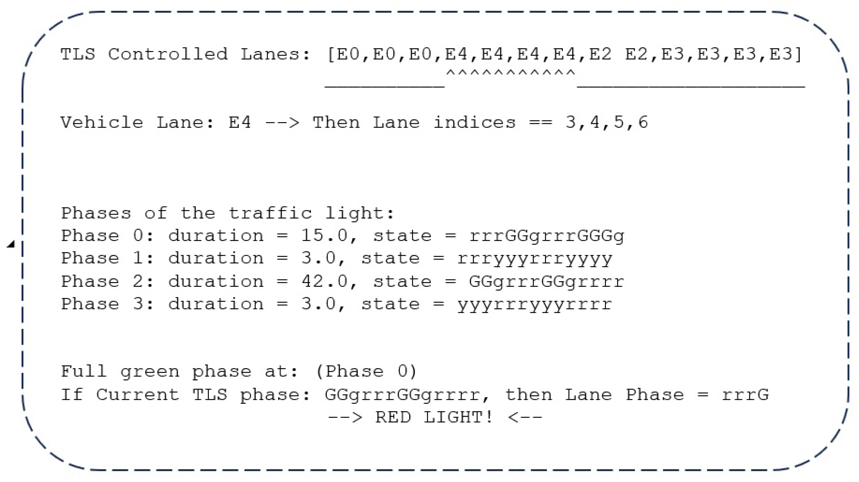
3.3.2. Retrieving the Actual Traffic Signal Phase
Initially, the program looks for where the green phase is, which allows platoon vehicles to proceed. Retrieving the green phase is achieved with the following algorithm sequence.
- Retrieve TLS-controlled lanes and the current vehicle lane;
- Loop over the TLS-controlled lanes and match the position (index) of the current vehicle lane;
- Retrieve this index, and store it;
- Retrieve the TLS complete logic program and then go through all available phases;
- Check where we have the green phase using the current vehicle lane index.
Figure 5 demonstrates an example of the TLS information retrieval with the SUMO TraCI code.
3.3.3. Situation Awareness
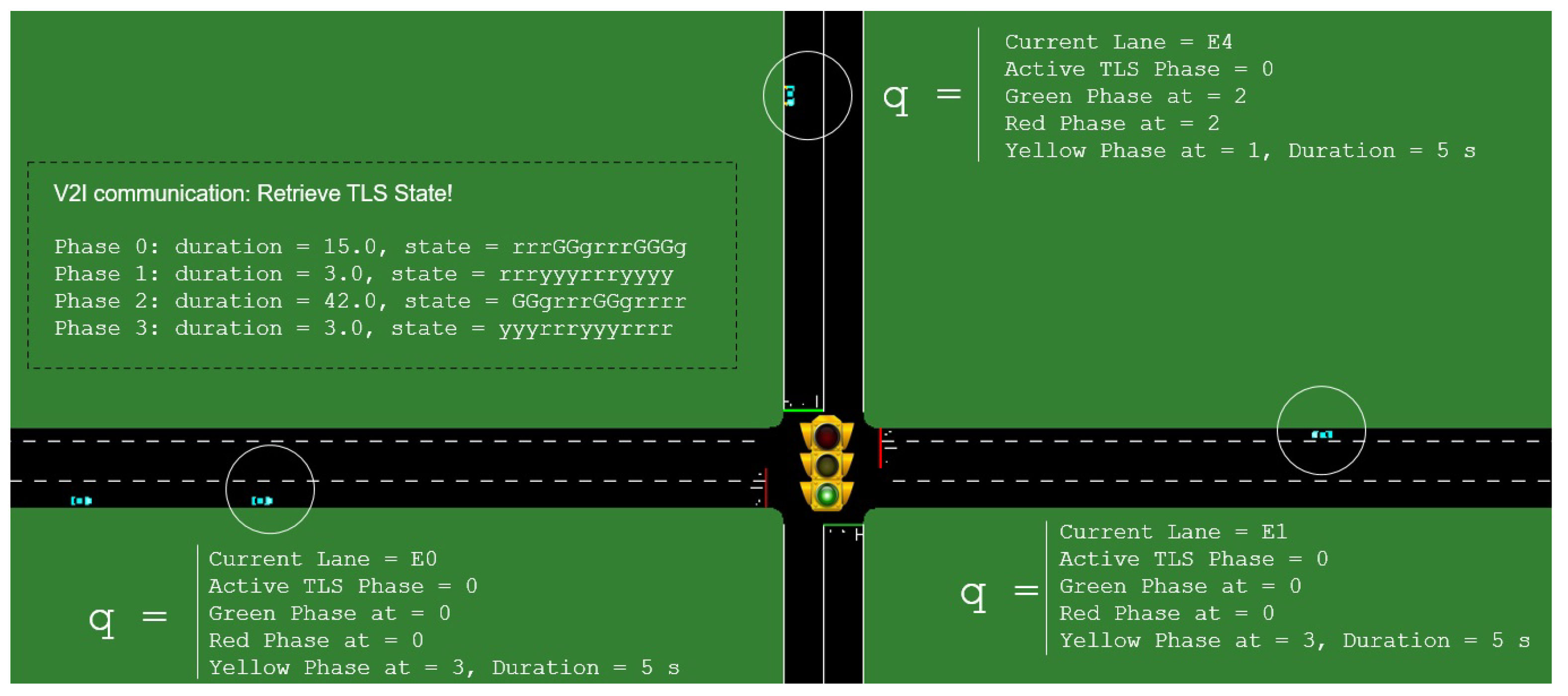
The situation awareness algorithm task is to recognize the whole intersection situation. In our case, we were dealing with TraCI commands, but in general, the task’s purpose is to identify for each vehicle approaching the traffic light the current traffic light state (more specifically to learn which phase has a green light, and in which phase the opposite lane has both red and yellow lights. Figure 6 represents the generated intersection configuration map for each approaching vehicle.
The algorithm’s output is comprehensive knowledge of the intersection’s traffic light conditions for the platoon’s lane and all other lanes. The platoon’s movements may be coordinated, and traffic flow may be optimized with the use of this data.
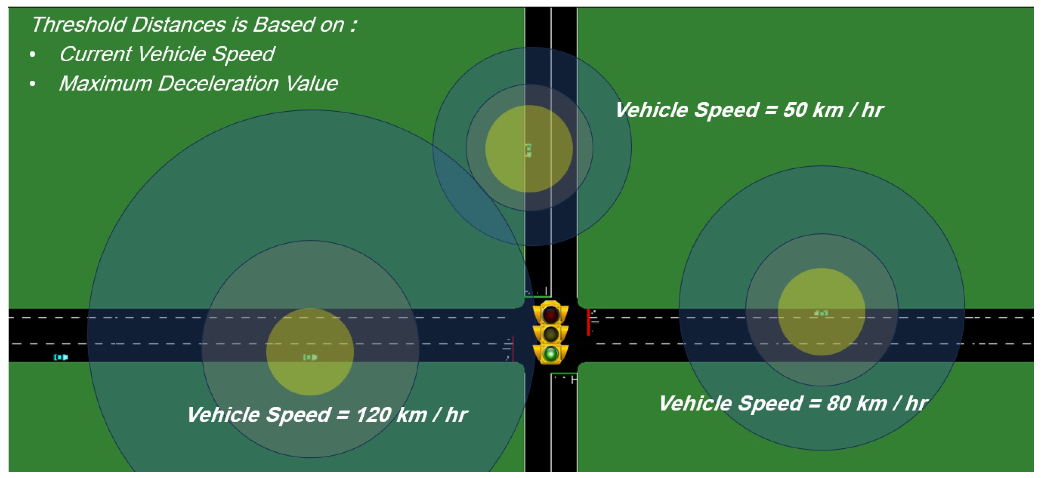
3.3.4. Calculating Distance Threshold
The primary procedure begins with the determination of a vehicle’s distance threshold in a simulated traffic environment. As a safety measure in the event of failed V2I communication, this threshold can be utilized to ascertain whether a vehicle can completely stop before approaching a red traffic light. Distance threshold represents the safest distance a car needs to perform a full stop in case of V2I communication failure. The first step is to obtain the current vehicle motion parameters, speed, and deceleration. Figure 7 represents the threshold distance calculation based on vehicle speed.
3.3.5. Traveled Distance (1)
Traveled distance (1) is the distance the vehicle would travel during the yellow light phase of the other lanes (the specific lane that we want to change its state from (green–yellow–red), depending on its speed :
3.3.6. Traveled Distance (2)
Traveled distance (2) is related to the distance a vehicle would travel during the moment when the driver starts to hit the brake pedals (we assume that the current deceleration is 0) until reaching maximum deceleration. Now, the generative deceleration value must be defined.
It is a “GENERATIVE VALUE” because it creates a value that an intelligent TLS needs to assist the intersection situation and to determine which vehicle takes priority in going through the intersection first.
The idea of the generative deceleration value refers to the amount of deceleration that a vehicle produces in response to particular driving circumstances. It stands for a vehicle’s ability to slow down quickly and effectively, which affects things like stopping distance, driver comfort, and overall safety. The braking system, tire traction, weight distribution, and other aspects unique to each vehicle all play a role in determining the generative deceleration value. The maximum deceleration the vehicle is capable of achieving during braking maneuvers is affected by all of these variables taken together. Controlled testing is carried out, sometimes on specialized tracks or controlled settings, where the vehicle’s braking ability is assessed under defined conditions in order to determine the generative deceleration value.
Driver errors are a common occurrence and must be considered, but it is challenging to predict the exact types and sources of these errors. The ability of a vehicle to slow down depends on both the driver’s skills and the vehicle’s capabilities. One practical solution to address this challenge is to measure deceleration based on historical records. Vehicles can keep records of a driver’s past behavior, including their typical deceleration when performing a full stop. By calculating the driver’s average deceleration in such situations, we can use this value as a reliable estimate. For the sake of simplicity, in this study, we have assumed that maximum deceleration is −4.5 m/s2.
Now, let us find the rate of change in deceleration (the situation where a driver decided to stop the moving vehicle car from a certain speed; in case the vehicle does not undergo either acceleration or deceleration, then m/s2):
The deceleration function is as follows:
where is assumed. Now, we need to calculate starting from applying deceleration until hitting the max deceleration, given the time period. It is assumed that normally, it will take 1 s to reach a maximum deceleration value (−4.5 m/s2), starting from 0 deceleration. It may look like the one-second calculations are not needed, but when we are talking about the dynamic traffic model for speeding up vehicles and considering a large network where we need to calculate precisely which vehicle takes priority in passing the intersection first, then this one-second time is very significant.
In order to calculate the traveled distance in this phase, where the vehicle undergoes a continuously changing deceleration (from 0 to −4.5 m/s2). First, we need to find the velocity function during this period by integrating the deceleration function, taking into account the initial (current) velocity:
Given that the initial speed at time 0 (m/s) is
the velocity function is as follows:
Now, we can find the reduced speed after reaching the maximum deceleration at t = time_period s, where we assumed t = 1:
Now, we integrate the velocity function to find the distance function “Used for Travelled Distance (2)”:
The constant D is irrelevant since we are interested in the traveled distance, as at time 0, the traveled distance is zero, so (we still have not applied the deceleration yet).
3.3.7. Traveled Distance (3)
From max deceleration until full stop: After reaching the maximum deceleration value, we will assume the perfect case; the vehicle will undergo a fixed deceleration value (applying the maximum = −4.5 m/s2), so this value will not change during the remaining stopping distance and will remain fixed. To calculate the traveled distance required for the vehicle to stop, we can use the following equation:
where
- u is the final velocity (0 m/s, as the vehicle stops);
- v is the reduced speed (m/s);
- a is the deceleration (Max_Deceleration_change m/s2);
- s is the traveled distance.
Thus, the vehicle would need to travel approximately meters to arrive at a complete stop given m/s, a = −4.5 m/s2. And finally, we can calculate the threshold distance for each moving vehicle:
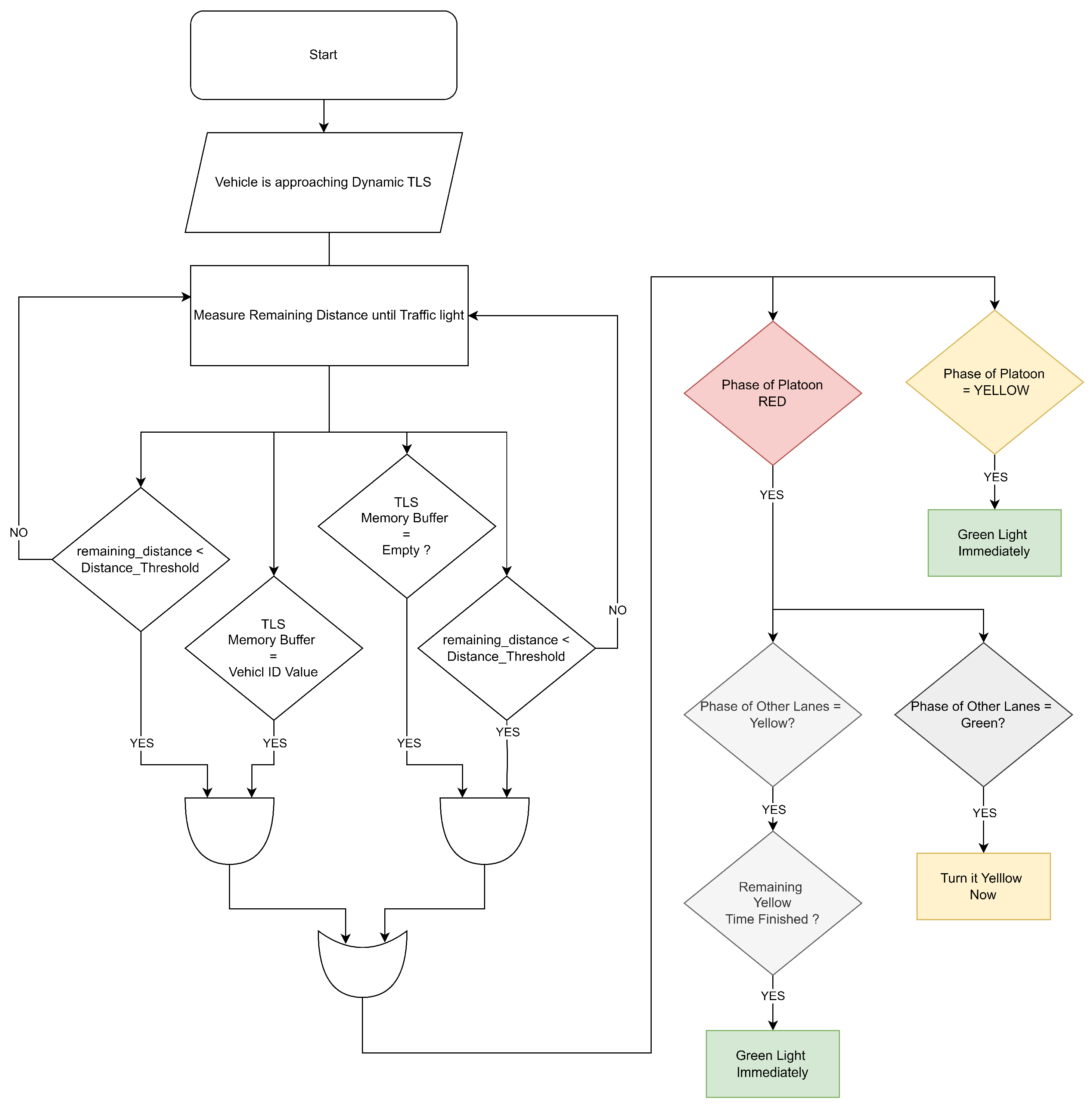
3.4. Initiating Green Traffic Light Phase (Main Algorithm)
If one of these conditions is met, then we can initiate the sequence of turning the green light on, where a complex condition in the “if-statement” compares two possibilities (TLS logic-gate-based decisions, see Figure 8: Making decisions based on which conditions are applied (TLS logic-gate-based decision).
- (Remaining distance < threshold) and (TLS buffer memory is empty).
- (Remaining distance < threshold) and (TLS buffer memory has the same ID as the vehicle).
The sequence of switching to the green light will be proposed considering the following procedure:
- If we have a yellow light, then initiate a green light.
- If we have a red light, then turn the traffic light of the other lanes to yellow immediately.
- After the yellow light is complete for the other lanes, then turn them immediately to red.
- Turn our traffic light to green if we meet all the possibilities.
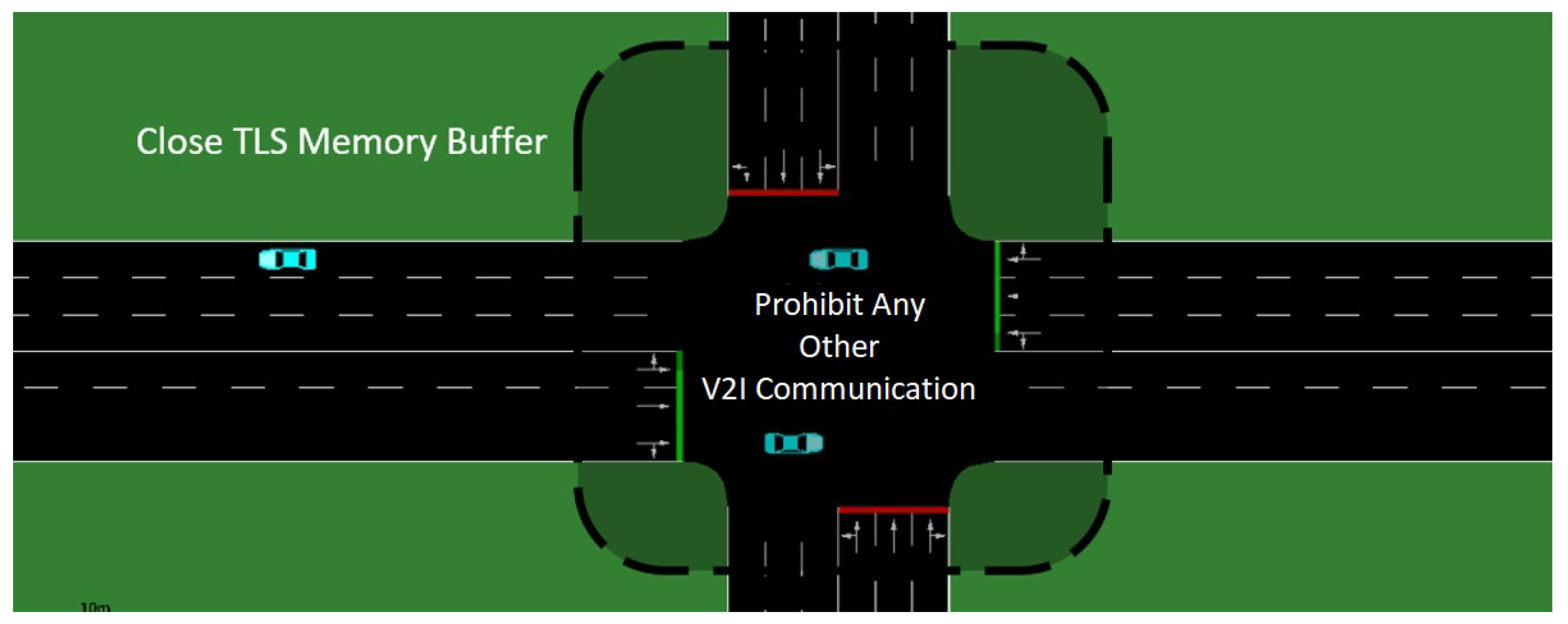
3.5. Introducing TLS Memory Buffer
TLS memory buffer is responsible for keeping only one vehicle in an active regulator state for the traffic light, i.e., no other vehicles can control the traffic light while there is active communication between the TLS and the given vehicle (see example in Figure 9). TLS memory buffer works according to the logic as follows:
- If a vehicle has initiated a V2I communication and it can control the TLS logic, then any other communication is blocked.
- If the vehicle has successfully passed the intersection, then the memory is wiped to allow other communication.
- If the actual communication has been lost, then then the memory is wiped to allow other communication.
4. Discussion
In this part, we discuss the test network configuration as well as the simulation-based performance testing.
4.1. Configuring Test Traffic Network
Budapest’s District XIV has been selected as the region of demonstration for assessing traffic characteristics and has been generated as a SUMO network. This area was chosen due to its suitability for researching traffic patterns and analyzing transportation systems. This is an urban environment that experiences significant vehicular and pedestrian traffic. In addition, this district has a complex road system with both major arterials and residential roads. This highly variable network topology permits the study of numerous traffic scenarios and the evaluation of traffic performance under varying environmental circumstances. The chosen area for testing is 2.3 km2, where the total road link length is 123.93 km, the total number of lanes is 1398, the total number of nodes 654 (we refer to intersections as nodes as we follow SUMO conventions; also, this number includes the network entrances and exits). Regarding traffic flow, vehicles generally maintain a smoother and more consistent pace, with decent levels of congestion and reduced delays compared with that at peak hours. Drivers can often travel at or near the posted speed limits, and there is generally a medium density of vehicles on the road, but allowing for convenient lane changes and merging, the number of signalized intersections is 16. In this test, we simulated 2135 vehicle trips.
4.2. Results
The main results of the simulations are tabulated into Table 1 and Table 2. Table 1 shows a significant improvement in the overall network testing parameters. Testing 2135 successful trips in a chosen network area, firstly by applying the dynamic traffic control algorithm, an improvement is obtained ranging from 14.7% to 36.11% in the performance metrics. These promising results are mainly due to the solution of a typical traffic problem, i.e., why should a vehicle stop at a traffic light waiting for its green light turn, while there are no other cars in the intersection? To resolve this issue, we applied the V2I technology, allowing the traffic signal to change to the green phase, in accordance with the discussed algorithm. In the second half of the table, more promising outcomes were achieved by applying both network platooning and Dynamic TLS. These results were obtained using the car dynamics to obtain higher speed to catch up to the platoon with the vehicles ahead. Thus, a faster overall network speed was obtained, such that the Dynamic TLS can allow for more cars to pass the green light, in contrast to the non-platooned cars that were driving separately, and waiting longer for their corresponding green light phase. With both platooning and Dynamic TLS, an improvement of 18.78% to 40.56% in performance metrics was achieved. Table 2 shows the accumulated average number of vehicles that were idling at the traffic light, meaning that those vehicles were caught by the red light and waiting for their green phase. We can see that in the uncontrolled case, an average of 6.8 vehicles were waiting at a red light, while in the controlled Dynamic TLS case, an average of 0.68 vehicles were waiting for the red light. Furthermore, every vehicle managed to pass the intersection in an organized way without waiting for the green light phase, i.e, the algorithm detected every vehicle moving towards the intersection and had an appropriate green phase to allow vehicles to pass the intersection effectively depending on its speed without delaying other vehicles in the intersection.
In general, smart intersections are complex systems whose effects may be felt in many areas of city life. The impact on traffic performance, congestion, road safety, environmental and economic considerations, and other areas must be evaluated for a whole picture of these crossings. Smart intersections help improve road safety by facilitating effective interaction among infrastructure elements, moving cars, and even pedestrians. Smart intersections may help the environment and the economy by decreasing emissions and fuel use by easing congestion at intersections. Progress towards smart intersections is challenging due to compatibility problems across systems and the high price tag of updating current infrastructure, i.e., technological and infrastructural obstacles must be overcome. Complicating matters even more are policy and legal concerns such as data privacy and liability in case of accidents. The future has many promising opportunities. There is a promise of improved traffic systems by leveraging artificial intelligence technology. Smart intersections will play an increasingly important role in controlling traffic flow as the prevalence of autonomous cars increases. Despite the challenges, adopting these high-tech solutions is crucial for creating safer and more efficient roads for everyone.
5. Conclusions
Our paper provided a technology to be implemented in future smart intersections. However, there are a number of technological and infrastructure issues that must be cleared before smart intersections can be put into real-world operation. The sophisticated technologies (sensors, communication devices, and data analytics platforms) utilized in these systems are very complicated to be implemented, integrated, and managed. Retrofitting old infrastructure with these new technologies might also provide significant financial and organizational challenges. The necessity for standardization to ensure interoperability, the deterioration of infrastructure, and maintenance problems are all major challenges.
Author Contributions
Conceptualization, H.A. and T.T.; methodology, H.A. and T.T.; simulation study, H.A.; validation, H.A.; writing—original draft preparation, H.A. and T.T.; writing review and editing, H.A., I.V. and T.T.; supervision, T.T.; project administration, I.V. All authors have read and agreed to the published version of the manuscript.
Funding
Project No. TKP2021-NVA-02 has been implemented with the support provided by the Ministry of Culture and Innovation of Hungary from the National Research, Development and Innovation Fund, financed under the TKP2021-NVA funding scheme. The research was supported by the European Union within the framework of the National Laboratory for Autonomous Systems (RRF-2.3.1-21-2022-00002).
Institutional Review Board Statement
Not applicable.
Informed Consent Statement
Not applicable.
Data Availability Statement
Not applicable.
Conflicts of Interest
The authors declare no conflict of interest.
Abbreviations
The following abbreviations are used in this manuscript:
| CACC | Cooperative Adaptive Cruise Control |
| C-V2X | Cellular vehicle-to-everything |
| DSRC | Dedicated Short Range Communication |
| AEB | Automatic emergency braking |
| GLODTA | Green Light Optimal Dwell Time Advisory |
| GLOSA | Green Light Optimal Speed Advisory |
| ITS | Intelligent Transport Systems |
| I2I | Infrastructure-to-infrastructure |
| Kp | Proportional gain parameter |
| Ki | Integral gain parameter |
| Kd | Derivative gain parameter |
| LIDAR | Light Detection and Ranging |
| PID | Proportional–Integral–Derivative |
| SPaT | Signal Phase and Timing |
| SUMO | Simulation of Urban Mobility |
| TLS | Traffic light system |
| TraCI | Traffic Control Interface |
| V2I | Vehicle-to-infrastructure |
| V2V | Vehicle-to-vehicle |
References
- Balador, A.; Bazzi, A.; Hernandez-Jayo, U.; de la Iglesia, I.; Ahmadvand, H. A survey on vehicular communication for cooperative truck platooning application. Veh. Commun. 2022, 35, 100460. [Google Scholar] [CrossRef]
- Fakhfakh, F.; Tounsi, M.; Mosbah, M. Vehicle platooning systems: Review, classification and validation strategies. Int. J. Netw. Distrib. Comput. 2020, 8, 203–213. [Google Scholar] [CrossRef]
- Kavathekar, P.; Chen, Y. Vehicle platooning: A brief survey and categorization. In Proceedings of the International Design Engineering Technical Conferences and Computers and Information in Engineering Conference, Washington, DC, USA, 28–31 August 2011; IEEE: Piscataway, NJ, USA, 2011; Volume 54808, pp. 829–845. [Google Scholar]
- Li, H.; Makkapati, V.P.; Wan, L.; Tomasch, E.; Hoschopf, H.; Eichberger, A. Validation of Automated Driving Function Based on the Apollo Platform: A Milestone for Simulation with Vehicle-in-the-Loop Testbed. Vehicles 2023, 5, 718–731. [Google Scholar] [CrossRef]
- Péter, T.; Szauter, F.; Rózsás, Z.; Lakatos, I. Integrated application of network traffic and intelligent driver models in the test laboratory analysis of autonomous vehicles and electric vehicles. Int. J. Heavy Veh. Syst. 2020, 27, 227. [Google Scholar] [CrossRef]
- Eom, M.; Kim, B.I. The traffic signal control problem for intersections: A review. Eur. Transp. Res. Rev. 2020, 12, 50. [Google Scholar] [CrossRef]
- Wágner, T.; Ormándi, T.; Tettamanti, T.; Varga, I. SPaT/MAP V2X communication between traffic light and vehicles and a realization with digital twin. Comput. Electr. Eng. 2023, 106, 108560. [Google Scholar] [CrossRef]
- Farkas, Z.; Mihály, A.; Gáspár, P. Analysis of Model Predictive Intersection Control for Autonomous Vehicles. Period. Polytech. Transp. Eng. 2023, 51, 209–215. [Google Scholar] [CrossRef]
- Islam, S.B.A.; Hajbabaie, A. Distributed coordinated signal timing optimization in connected transportation networks. Transp. Res. Part C Emerg. Technol. 2017, 80, 272–285. [Google Scholar] [CrossRef]
- Altan, O.D.; Wu, G.; Barth, M.J.; Boriboonsomsin, K.; Stark, J.A. GlidePath: Eco-Friendly Automated Approach and Departure at Signalized Intersections. IEEE Trans. Intell. Veh. 2017, 2, 266–277. [Google Scholar] [CrossRef]
- Liu, H.; Lu, X.Y.; Shladover, S.E. Traffic signal control by leveraging Cooperative Adaptive Cruise Control (CACC) vehicle platooning capabilities. Transp. Res. Part C Emerg. Technol. 2019, 104, 390–407. [Google Scholar] [CrossRef]
- ETSI. ETSI TS 103 191-3 V1.1.1 (2015-09); Technical Report; European Telecommunications Standards Institute: Valbonne, France, 2015. [Google Scholar]
- Kenney, J.B. Dedicated short-range communications (DSRC) standards in the United States. Proc. IEEE 2011, 99, 1162–1182. [Google Scholar] [CrossRef]
- Dey, K.C.; Yan, L.; Wang, X.; Wang, Y.; Shen, H.; Chowdhury, M.; Yu, L.; Qiu, C.; Soundararaj, V. A review of communication, driver characteristics, and controls aspects of cooperative adaptive cruise control (CACC). IEEE Trans. Intell. Transp. Syst. 2015, 17, 491–509. [Google Scholar] [CrossRef]
- Kospach, A.; Irrenfried, C. Truck Platoon Slipstream Effects Assessment. In Energy-Efficient and Semi-Automated Truck Platooning: Research and Evaluation; Springer International Publishing: Cham, Switzerland, 2022; pp. 57–68. [Google Scholar]
- Ziebinski, A.; Cupek, R.; Erdogan, H.; Waechter, S. A survey of ADAS technologies for the future perspective of sensor fusion. In Proceedings of the Computational Collective Intelligence: 8th International Conference, ICCCI 2016, Halkidiki, Greece, 28–30 September 2016; Proceedings, Part II 8. Springer: Cham, Switzerland, 2016; pp. 135–146. [Google Scholar]
- Kocić, J.; Jovičić, N.; Drndarević, V. Sensors and sensor fusion in autonomous vehicles. In Proceedings of the 2018 26th Telecommunications Forum (TELFOR), Belgrade, Serbia, 20–21 November 2018; pp. 420–425. [Google Scholar]
- Chavez-Garcia, R.O.; Aycard, O. Multiple sensor fusion and classification for moving object detection and tracking. IEEE Trans. Intell. Transp. Syst. 2015, 17, 525–534. [Google Scholar] [CrossRef]
- Bayuwindra, A.; Ploeg, J.; Lefeber, E.; Nijmeijer, H. Combined longitudinal and lateral control of car-like vehicle platooning with extended look-ahead. IEEE Trans. Control Syst. Technol. 2019, 28, 790–803. [Google Scholar] [CrossRef]
- Cseh, C. Architecture of the dedicated short-range communications (DSRC) protocol. In Proceedings of the VTC’98, 48th IEEE Vehicular Technology Conference, Pathway to Global Wireless Revolution (Cat. No. 98CH36151), Ottawa, ON, Canada, 18–21 May 1998; Pathway to Global Wireless Revolution (Cat. No. 98CH36151). Volume 3, pp. 2095–2099. [Google Scholar]
- Eichler, S. Performance evaluation of the IEEE 802.11pWAVE communication standard. In Proceedings of the 2007 IEEE 66th Vehicular Technology Conference, Baltimore, MD, USA, 30 September–3 October 2007; pp. 2199–2203. [Google Scholar]
- Seredynski, M.; Khadraoui, D. Complementing Transit Signal Priority with speed and dwell time extension advisories. In Proceedings of the 17th International IEEE Conference on Intelligent Transportation Systems (ITSC), Qingdao, China, 8–11 October 2014; pp. 1009–1014. [Google Scholar]
- Seredynski, M.; Khadraoui, D.; Viti, F. Signal phase and timing (SPaT) for cooperative public transport priority measures. In Proceedings of the 22nd ITS World Congress, Bordeaux, France, 5–9 October 2015. [Google Scholar]
- Lopez, P.A.; Behrisch, M.; Bieker-Walz, L.; Erdmann, J.; Flötteröd, Y.P.; Hilbrich, R.; Lücken, L.; Rummel, J.; Wagner, P.; Wießner, E. Microscopic Traffic Simulation using SUMO. In Proceedings of the 21st IEEE International Conference on Intelligent Transportation Systems, Maui, HI, USA, 4–7 November 2018. [Google Scholar]
Figure 1.
Platooning architecture flowchart.

Figure 2.
Platooning PID algorithm flowchart.

Figure 3.
Example for internal clearance distance.

Figure 4.
Effect of clearance to the platoon performance metrics.

Figure 5.
TraCI TLS logic information example.

Figure 6.
Generated intersection configuration map—V2I.

Figure 7.
Effect of vehicle speed on threshold distance.

Figure 8.
The flowchart of the TLS logic.

Figure 9.
TLS memory buffer information example.


Table 1.
Test results.
| Simulation Statistics | |
|---|---|
| UNCONTROLLED CASE | |
| The traveling time of the platoon is 8578 [s] | |
| The overall fuel consumption is 866,626,097.28 [mL] | |
| The overall CO emission is 71,042,916.87 [mg] | |
| The overall CO2 emission is 2,717,031,380.17 [mg] | |
| The overall NOx emission is 1,110,266.32 [mg] | |
| The total absolute acceleration is 811,577.89 [m/s2] | |
| Percentage Saving % | |
| CONTROLLED CASE (Dynamic TLS control Only) | |
| The traveling time of the platoon is 7315 [s] | 14.72% |
| The overall fuel consumption is 717,236,540.47 [mL] | 17.24% |
| The overall CO emission is 45,389,785.52 [mg] | 36.11% |
| The overall CO2 emission is 2,248,682,109.77 [mg] | 17.24% |
| The overall NOx emission is 893,782.28 [mg] | 19.50% |
| The total absolute acceleration is 683,700.15 [m/s2] | 15.76% |
| CONTROLLED CASE (Network Platooning + Dynamic TLS) | |
| The traveling time of the platoon is 6967 [s] | 18.78% |
| The overall fuel consumption is 707,217,302.56 [mL] | 18.39% |
| The overall CO emission is 42,226,608.01 [mg] | 40.56% |
| The overall CO2 emission is 2,217,274,631.53 [mg] | 18.39% |
| The overall NOx emission is 880,294.35 [mg] | 20.71% |
| The total absolute acceleration is 696,407.48 [m/s2] | 14.19% |
Table 2.
Average network speed and halt index.
| Average Network Speed | Average Number of Stopped Vehicles/Intersection (Halt Index) | |
|---|---|---|
| Uncontrolled Speed | 33.52 km/h | 6.8 |
| Controlled Speed | 37.22 km/h (+9.2%) | 0.68 +90% Improvement |
Disclaimer/Publisher’s Note: The statements, opinions and data contained in all publications are solely those of the individual author(s) and contributor(s) and not of MDPI and/or the editor(s). MDPI and/or the editor(s) disclaim responsibility for any injury to people or property resulting from any ideas, methods, instructions or products referred to in the content. |
© 2023 by the authors. Licensee MDPI, Basel, Switzerland. This article is an open access article distributed under the terms and conditions of the Creative Commons Attribution (CC BY) license (https://creativecommons.org/licenses/by/4.0/).
Share and Cite
MDPI and ACS Style
Altamimi, H.; Varga, I.; Tettamanti, T. Urban Platooning Combined with Dynamic Traffic Lights. Machines 2023, 11, 920. https://doi.org/10.3390/machines11090920
AMA Style
Altamimi H, Varga I, Tettamanti T. Urban Platooning Combined with Dynamic Traffic Lights. Machines. 2023; 11(9):920. https://doi.org/10.3390/machines11090920
Chicago/Turabian StyleAltamimi, Husam, István Varga, and Tamás Tettamanti. 2023. "Urban Platooning Combined with Dynamic Traffic Lights" Machines 11, no. 9: 920. https://doi.org/10.3390/machines11090920
Note that from the first issue of 2016, this journal uses article numbers instead of page numbers. See further details here.