A Deep Learning Framework for Intelligent Fault Diagnosis Using AutoML-CNN and Image-like Data Fusion

Abstract

Intelligent fault diagnosis (IFD) is essential for preventative maintenance (PM) in Industry 4.0. Data-driven approaches have been widely accepted for IFD in smart manufacturing, and various deep learning (DL) models have been developed for different datasets and scenarios. However, an automatic and unified DL framework for developing IFD applications is still required. Hence, this work proposes an efficient framework integrating popular convolutional neural networks (CNNs) for IFD based on time-series data by leveraging automated machine learning (AutoML) and image-like data fusion. After normalisation, uniaxial or triaxial signals are reconstructed into -channel pseudo-images to satisfy the input requirements for CNNs and achieve data-level fusion simultaneously. Then, the model training, hyperparameter optimisation, and evaluation can be taken automatically based on AutoML. Finally, the selected model can be deployed on a cloud server or an edge device (via tiny machine learning). The proposed framework and method were validated via two case studies, demonstrating the framework’s availability for the automatic development of IFD applications and the effectiveness of the proposed data-level fusion method.

1. Introduction

Intelligent fault diagnosis (IFD) [1] plays a vital role in preventative maintenance (PM) for Industry 4.0, which can reduce downtime, improve overall system efficiency, decrease maintenance costs, enhance reliability, and extend the lifespan of machinery, as well as help to optimise operations and make informed decisions. Data-driven approaches based on deep learning (DL) have been widely accepted for IFD in smart manufacturing. Meanwhile, various deep neural network (DNN) architectures have been utilised and developed in the field of IFD. However, these DL models are usually isolated, and previous efforts [2,3,4,5,6] have always focused on creating a single DNN architecture for a specific dataset or working scenario, which does not consider comparative analysis of these models. Hence, an automatic and unified DL framework for IFD development is still required, which comprises automatic data fusion, model training, hyperparameter optimisation, and evaluation.

This work proposes an efficient IFD framework integrating popular convolutional neural networks (CNNs) for time-series data by leveraging automated machine learning (AutoML) and image-like data fusion. After normalisation, the uniaxial or triaxial signals can be reshaped into 3-channel pseudo-images through the proposed phase space reconstruction, satisfying the input requirements for CNNs and achieving data fusion simultaneously. With the reconstructed 3-channel pseudo-images, model training can be carried out automatically via the integrated CNN architectures based on AutoML. Then, the trained models are evaluated automatically according to different metrics, including accuracy, precision, recall, F1 score, ROC, AUC, MCC, FLOPs, and the model parameters. Finally, the selected model can be deployed on a cloud server or an edge device via tiny machine learning (tinyML) for practical applications, such as in a digital-twin (DT) manufacturing system, which requires efficient and resilient decision-making, even under communication-constraint circumstances.

The proposed framework and data fusion method were validated via two case studies using uniaxial and triaxial vibration signals. The experiments demonstrate that the proposed framework leveraging AutoML-CNN can automatically realise model training and evaluation, which enhances the development efficiency for IFD applications. Moreover, it proves that the fused triaxial data through the proposed data-level fusion can perform better than the single-axis data using the same neural network. The main contribution of this study is two-fold: (1) it proposes an efficient and automatic framework for IFD development by leveraging AutoML-CNN and (2) it proposes an image-like data-level fusion method to handle triaxial time-series signals.

The rest of this paper is structured as follows: Section 2 overviews the related work for IFD based on machine learning. Section 3 presents the proposed pseudo-image reconstruction method and the IFD framework. Section 4 is the framework validation via case studies. Section 5 concludes the work and discusses the future research direction.

2. Related Works

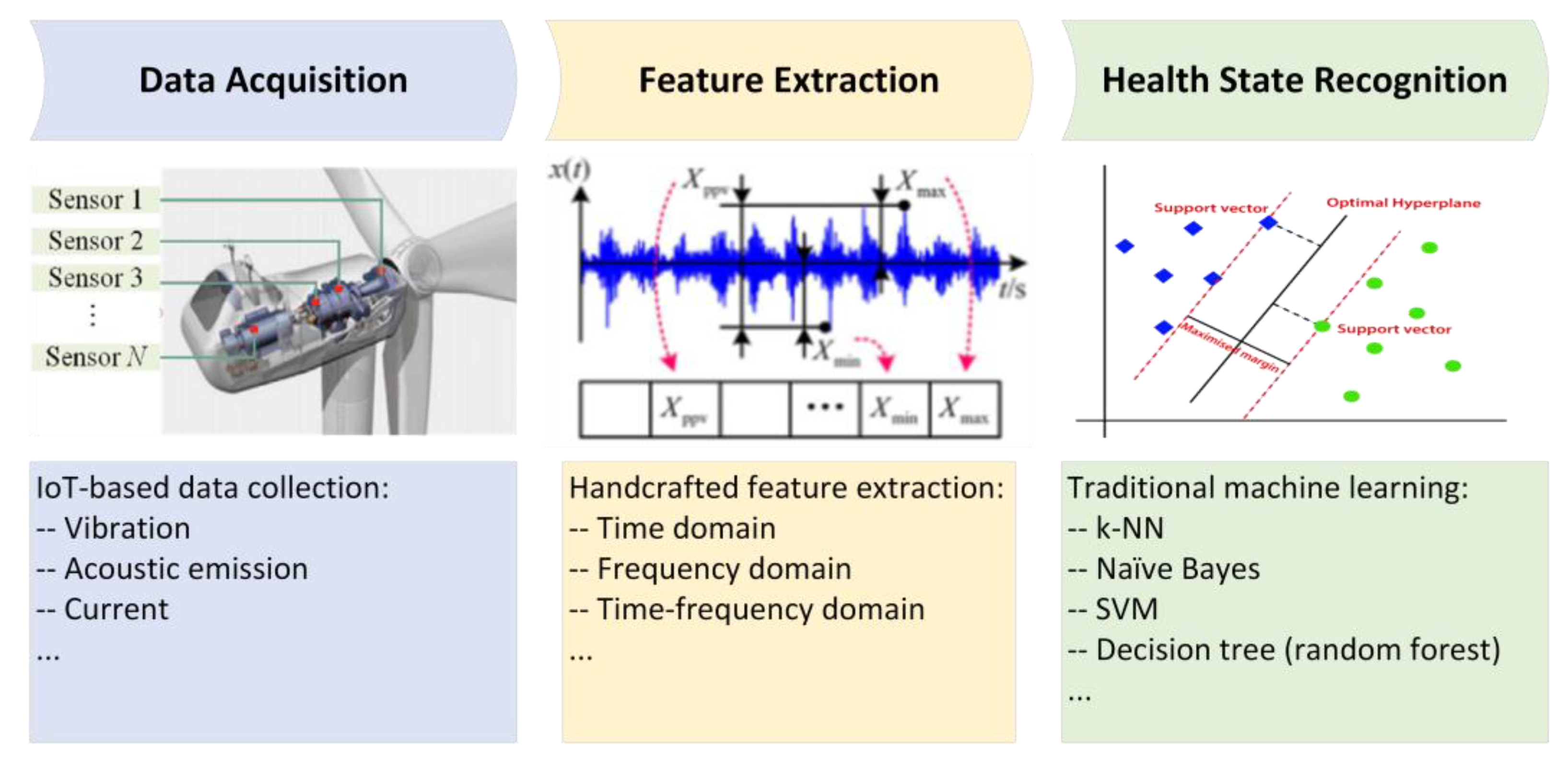
2.1. IFD with Traditional Machine Learning

Intelligent fault diagnosis (IFD) methods that can automatically recognise the health states of machines and infrastructures [7] are essential for preventative maintenance in Industry 4.0. Many traditional machine learning (ML) approaches can be applied in IFD, such as k-nearest Neighbour (k-NN) [8], Naïve Bayes classifier [9], support vector machine (SVM) [10], decision tree [11], and random forests [12], etc., which rely on manual features. The pipeline for IFD based on traditional ML can be condensed as shown in Figure 1, which starts from data acquisition through various IoT technologies to feature extraction via handcrafted design and automatic data-driven health state recognition using supervised or unsupervised learning approaches.

Data for fault diagnosis are usually in time series and collected constantly from different sensors mounted on machines or infrastructures, such as acceleration, displacement, strain, and acoustic signals, as well as ambient conditions like temperature and wind speed. The commonly used features can be categorised into time, frequency, and time–frequency domains based on the extraction methods, e.g., the statistical features, zero-cross rate, wavelet, fractal features in the time domain, discrete Fourier transform (DFT), and power spectral density (PSD) in the frequency domain; energy and entropy from short-term Fourier transform (STFT), wavelet transform (WT), wave packet transform (WPT), and Hilbert–Huang transform (HHT) in the time–frequency domain, as shown in

Table 1. Traditional machine learning pipeline for IFD.

Machine Learning	Handcrafted Feature Extraction	Approaches
Traditional ML	Time domain: statistical features, zero-cross rate, wavelet, fractal features, etc.	KNN, SVM, Naïve Bayes classifier, decision tree, random forest, etc.
	Frequency domain: DFT, PSD, etc.
	Time–frequency domain: STFT, WT, WPT, EMD, HTT, etc.

.

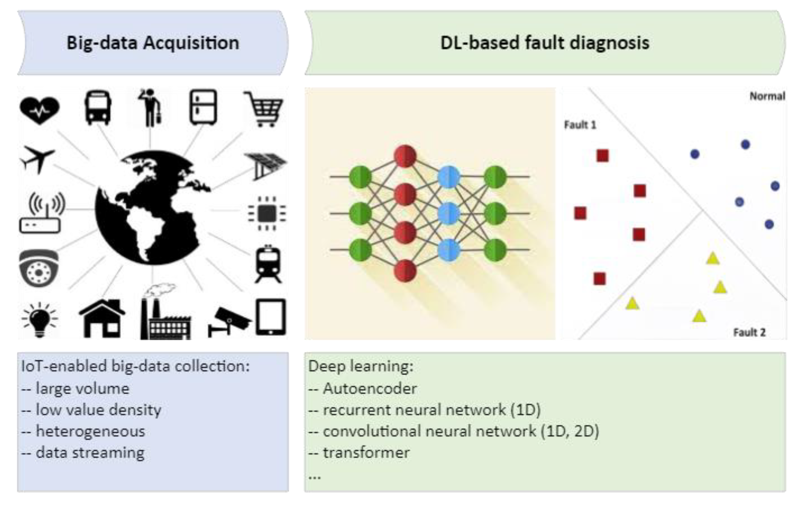
2.2. IFD with Deep Learning

With the rapid development of the IoT, the collected data volume is dramatically higher than ever before and brings more useful information for fault diagnosis. Big data acquisition has four characteristics: volume, quality, variety, and velocity [7].

(1)

Volume—the volume of collected data sustainably grows during the long-term operation and maintenance (O&M).

(2)

Quality—a portion of poor-quality data is mingled in the massive data.

(3)

Variety—multi-source data is collected from multiple sources (by different sensors) with a heterogeneous structure.

(4)

Velocity—fast transmission can be enabled in situ via fieldbus cables or at the remote end via high-speed communication like 5G, which promises response and decision-making in near real-time for DT.

Traditional ML relying on handcrafted features becomes inappropriate for big data scenarios. Hence, IFD has been extensively developed based on DL, which can learn features automatically. Its pipeline is shown in Figure 2, consisting of only two steps, i.e., data acquisition and health state recognition, which can accommodate massive data and achieve a higher level of automation by skipping the step of manual feature extraction. The widely used DL approaches for IFD include multilayer perceptron (MLP), autoencoder (AE), recurrent neural network (RNN), convolutional neural network (CNN), transformer, etc.

2.2.1. DL with 1D Time Series

Liu et al. [13] and Lu et al. [14] employed the stacked sparse AE and the stacked denoising AE for the IFD of bearings, presenting higher diagnosis accuracy than traditional ML methods. Common RNNs, including gated recurrent units (GRUs) and long-term memory networks (LSTM), are theoretically an ideal non-linear time-series forecasting tool and a universal approximator for dynamic systems [15]. Ling et al. [16] employed RNN to achieve early warning in the fault creep period for nuclear power machinery, together with principal component analysis (PCA), wavelet analysis, and Bayesian inference. Yuan et al. [17] utilised LSTM for IFD and remaining useful life (RUL) estimation for aero-engine based on time-series data. Moreover, Neves et al. [18,19] employed an MLP with train-induced acceleration data to identify the structure health conditions of the KW51 railway bridge. Sajedi and Liang [20] proposed a framework based on a fully convolutional encoder–decoder architecture for structural damage diagnosis with the vibration signals from a grid sensor network, which can localise damages and distinguish multiple damage mechanisms with reliable generalisation capacities.

Additionally, 1D-CNN is also inherently suitable for time-series pattern recognition. For example, Wu et al. [21] proposed an approach for rub-impact fault diagnosis of a rotor system based on 1D-CNN. Sony et al. [22] designed a 1D-CNN to identify multiclass damage using bridge vibration data. 1D CNN was also utilised to detect the change of local structural stiffness and mass based on acceleration from a single sensor [23,24].

2.2.2. DL with 2D Synthetic Images

As the monitoring variable for IFD is usually a 1D time series, which is different from 2D images, to leverage the powerful feature learning capability of CNNs, many efforts have been made to transform 1D motion signals into 2D images, including Gramian angular field (GAF) [25], wavelet transform [26,27,28], S-transform [29], phase space reconstruction [30], etc. The GAF, wavelet transform, and S-transform are time-consuming, and the latter two require expert knowledge in the frequency domain for spectrum exploration. In contrast, phase space reconstruction can quickly generate synthetic images with simple backgrounds. For example, time series can be converted through Equation (1) (i.e., min–max normalisation) into a single-channel greyscale image, as shown in Figure 3.

$$P\left(j,k\right)=\mathit{round}\left\{\frac{f\left(x\left(\left(j-1\right)\times L+k\right)-\mathit{Min}(f\left(x\right)\right)}{\mathit{Max}(f\left(x\right))-\mathit{Min}(f(x\left)\right)}\times 255\right\}$$

(1)

where $P(j,k)\in [0,255]$ denotes the pixel strength of the grayscale image and j and k are the row and column numbers in the reconstructed image, respectively.

The DL-based IFD can be summarised as shown in

Table 2. Deep learning pipeline for IFD.

Pipeline	Approaches
Deep Learning	1D time series: RNN (including GRU and LSTM), 1D-CNN, etc.
	2D synthetic images: (1) Imaging—GAF, wavelet transform, S-transform, phase space reconstruction, etc. (2) Models—shallow single-channel CNNs and classical three-channel deep CNNs via proposed imaging.

. Previous works [30,31,32] have already proved the effectiveness of using shallow CNNs, like modified LeNet, for IFD. However, they mainly focused on a single sensor and did not consider data fusion for the signals from triple sensors or axes. Meanwhile, the imaging method has not been further developed to generate three-channel images (like RGB) to take advantage of the popular deep CNN architectures.

2.3. IFD with Data Fusion

Data fusion is usually employed in IFD based on multi-sensor data, which is supposed to be an effective way to improve pattern recognition accuracy. It includes data-level and decision-level fusion. Teng et al. [33] trained seven individual 1D CNNs using the acceleration signals from the corresponding sensors and fused their classification results at the decision level by hard voting. Compared with data-level fusion, i.e., integrating all acceleration signals into a multi-channel time sequence, decision-level fusion enhanced the classification accuracy by at least 10% in the experiments. However, this comparison consequence is not absolute. For example, Gao et al. [34] trained a single 1D CNN with the data-level fused acceleration signals from six sensors on a bridge for structure health-state recognition. Compared with decision-level fusion with hard and soft voting from six individual classifiers, data-level fusion can enhance the test accuracy by more than 20%. Furthermore, Gong et al. [35] used multi-channel data-level fusion of time-series signals from different sensors for the IFD of rotating machinery by leveraging CNN-SVM, which also achieves excellent test performance (nearly 100% accuracy). As can be seen, the level of fusion occurrence in IFD is flexible, depending on the used dataset and the selected neural network architecture.

3. Proposed IFD via AutoML-CNN and Image-like Fusion

3.1. Problem Statement

As can be seen from the related works for IFD with deep learning, CNN-based pattern recognition using the derived 2D images from time-series data has become one of the most effective approaches for data-driven fault diagnosis. It can be attributed to the excellent feature learning capability of CNNs and subsequent fully connected networks’ (FCNs) fitting ability. Meanwhile, there are already many classical CNN architectures designed in computer vision, including LeNet, VGG, ResNet, EfficientNet, MobileNet, etc., as well as techniques developed for improvement, such as dilated convolution, attention, and lightweight design.

However, previous research has usually focused on implementing or improving an individual architecture, such as modified LeNet, VGG16, and transformer. Still, it did not involve different neural networks in a unified framework by leveraging AutoML. As is known, variant neural networks could perform differently in data-driven fault diagnosis even for the same dataset. Therefore, how to automatically realise training (including parameter optimisation) and select the most appropriate neural network has become an issue for developing practical IFD applications. Meanwhile, how to fuse the data from a triaxial sensor, such as three-axis acceleration on (x, y, z), efficiently and effectively is also a problem.

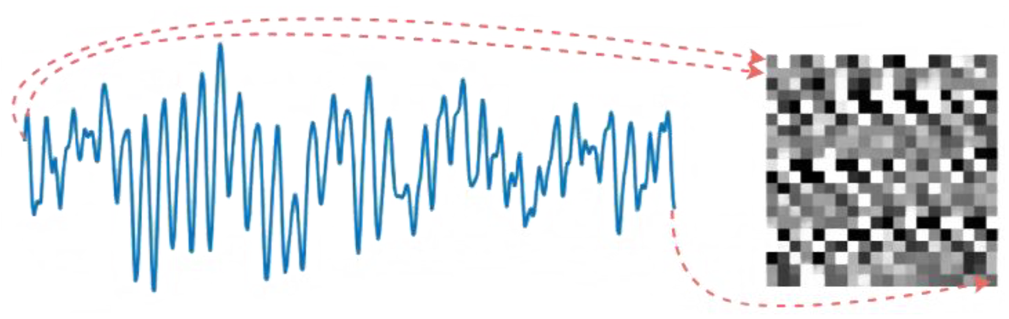
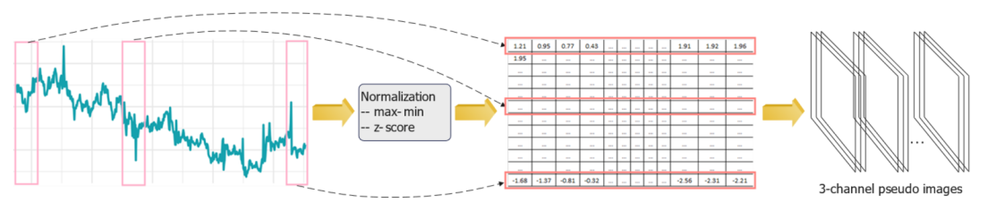
3.2. Pseudo-Image Reconstruction and Data Fusion

The previous time–frequency transformation from 1D time-series signals to 2D synthetic images is usually time-consuming (e.g., the wavelet transformation for a sliding window of 1032 will take 1.653 s on Google Colab) and requires expert knowledge of the frequency spectrum. In contrast, the spatial reconstruction from the same time-series sliding window to a grayscale image like in [30] will only take 0.0001 s. However, the generated single-channel grayscale image cannot be utilised directly as input for the popular deep CNNs because they are designed for three-channel RGB images. Hence, an improved three-channel pseudo-image reconstruction (i.e., imaging) method is proposed here, as shown in Figure 4.

The first step in pre-process is to select an appropriate sliding window size, which depends on the sampling frequency, computing capability (for edge device), etc. Normalisation is suggested to decrease the time cost of training convergence, which can be the min–max normalisation or z-score standardisation of the training data. The pseudo-image pixels (i.e., matrix element) can be decimals without scaling up to the range of [0, 255] (i.e., unlike Equation (1) in previous research) because neural networks can convert the decimals to the scores between [0, 1] after the hidden layers and softmax functions. The slice of signals on each axis is reshaped as a single-channel pseudo-image in rows or columns, as shown in Figure 3. Then, the single-channel pseudo-image from a uniaxial signal can be duplicated to three channels, and the slice of triaxial signals can be reconstructed into a three-channel pseudo-image by stacking the single-channel image from each axis, as shown in Figure 4. The latter can achieve triaxial data-level fusion and satisfy the input requirement for CNN architectures at the same time.

3.3. Automated Machine Learning

Automated machine learning (AutoML) includes the end-to-end procedure from beginning with a raw dataset to building a machine learning model ready for deployment. The high degree of automation in AutoML aims to allow non-experts to use machine learning models and techniques without requiring them to become experts in machine learning [36]. Currently, most popular CNN architectures have already been built as APIs in the mainstream DL framework, including Keras, TensorFlow, PyTorch, etc. They can be revoked straightforwardly, which serves as the foundation of AutoML in this study.

After the proposed imaging, the derived three-channel pseudo-images are adopted as the input for integrated DL neural networks, which can be the built-in classical CNN architectures or the self-defined models. It is worth noting that the integrated neural networks are not limited to CNNs and can be any DNN architecture designed for RGB images, such as the Swim Transformer. The pseudo-images need to be resized appropriately according to the input requirement of each neural network. Then, the AutoML procedure can be carried out as shown in Figure 5, consisting of (1) automatic training through the popular DL frameworks for the integrated CNN architectures; (2) neural network search (and hyperparameter optimisation) based on evaluation according to various metrics; and (3) deployment on an edge device through tinyML.

Notably, the first two steps are supposed to be taken on a high-performance computer, such as a cloud server with a GPU, because DL training requires considerable computing power and memory. Hyperparameters, including optimiser, epoch, activation function, and learning rate, are also available for automatic optimisation via different approaches, such as random search, grid search, Hyperband [37], Bayesian hyperparameter optimisation (BHO) [38], tree-structured Parzen estimator (TPE) [39], population-based training (PBT) [40]. Appropriate transfer learning, such as pre-trained backbones from similar signals, can also be integrated into the training step, especially when applying self-defined neural networks.

The models were evaluated via different metrics (see Equations (2)–(7)), including accuracy, precision, recall, F1 score, receiver operating characteristic curve (ROC), area under the ROC curve (AUC), Matthew’s correlation coefficient (MCC), etc.

where TP—true positive, TN—true negative, FP—false positive, and FN—false negative.

$$\mathrm{Accuracy}=\frac{TN+TP}{TN+FP+TP+FN}$$

(2)

$$\mathrm{Precision}=\frac{TP}{TP+FP}$$

(3)

$$\mathrm{Recall}=\frac{TP}{TP+FN}$$

(4)

$$F1\mathrm{Score}=2\ast \frac{\mathrm{Precision}\ast \mathrm{Recall}}{\mathrm{Precision}+\mathrm{Recall}}$$

(5)

$$\mathrm{MCC}=\frac{TP\times TN-FP\times FN}{\sqrt{\left(TP+FP\right)\left(TP+FN\right)\left(TN+FP\right)\left(TN+FN\right)}}$$

(6)

$$AUC=\frac{\sum {\left(p_i,n_j\right)}_{p_i>n_j}}{P\ast N}$$

(7)

where $P$—the number of positive examples; $N$—the number of negative examples; $p_i$—the prediction score for a positive example; and $n_j$—the prediction score for a negative example.

Additionally, because the float point operations (FLOPs) represent the forward-pass computing capability needed by the neural network model, the number of model parameters (params) is subject to the computing memory, and the frame per second (FPS) reflects the processing speed; if the trained models have similar performance using the above indicators, the one with fewer FLOPs, fewer params, and higher FPS would be recommended for practical applications.

Finally, the selected DL model can be deployed on edge devices for IFD by leveraging tinyML, such as TensorFlow Lite. Moreover, as edge devices are also usually the equipment for data acquisition or aggregation, the newly collected data can be used to update the training set based on supervised or semi-supervised learning via appropriate annotation, thereby enhancing the long-term performance of the IFD application, as shown as the loop in Figure 5.

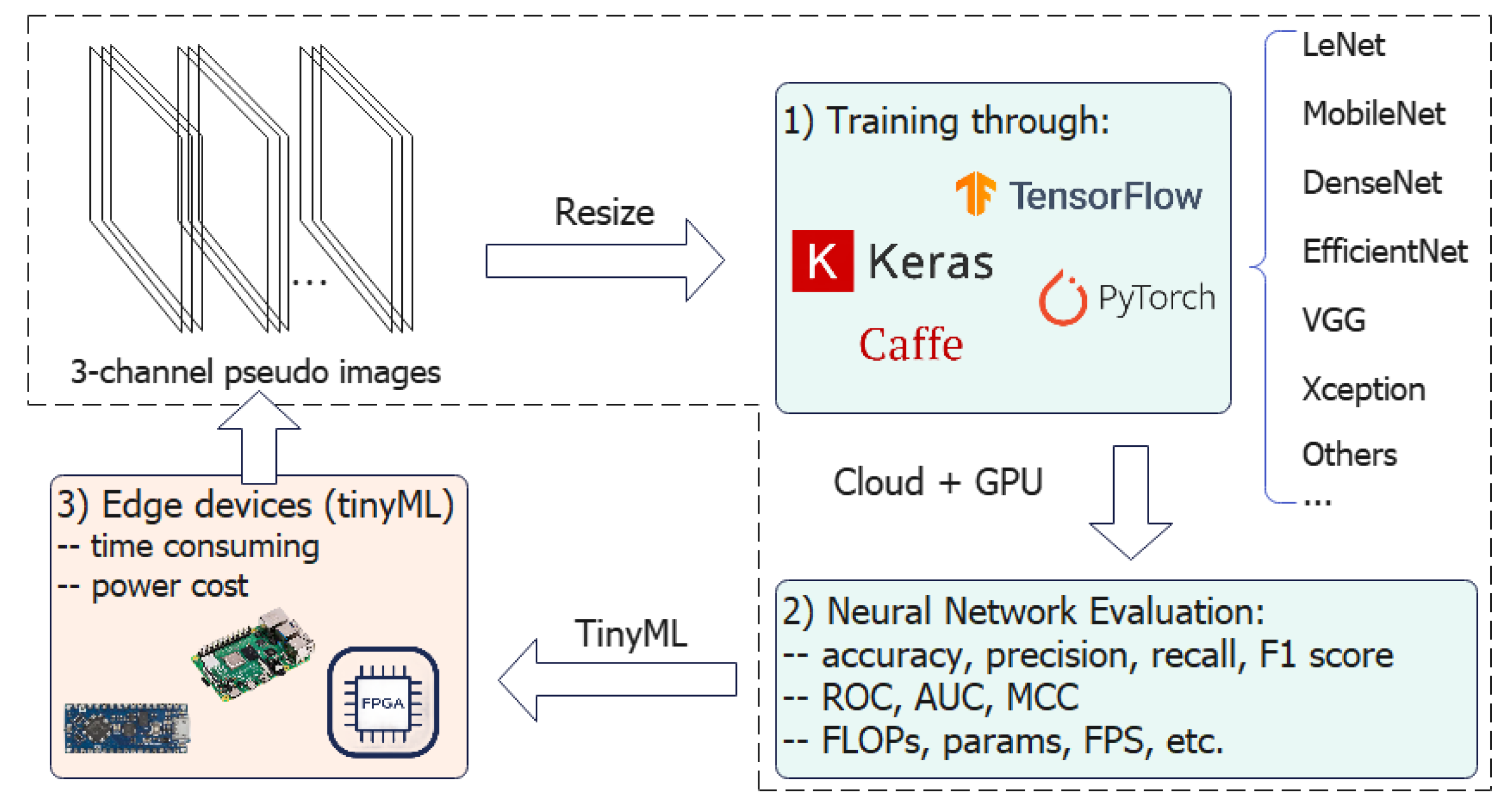
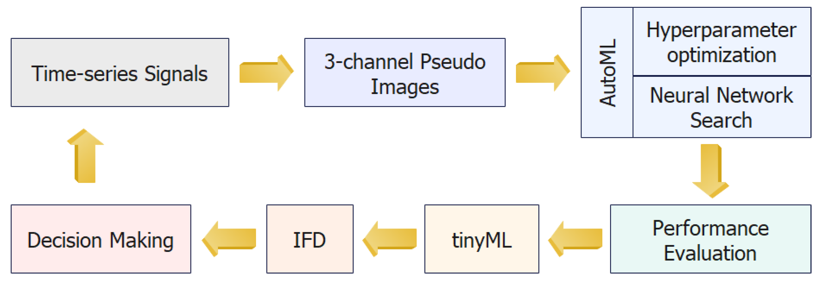
3.4. Proposed Framework and Workflow

The complete workflow for IFD by leveraging AutoML-CNN and image-like data fusion can be seen in Figure 6. The time-series signals from uniaxial and triaxial sensors are adopted as the input for the built-in and self-defined CNN architectures seamlessly after the proposed pseudo-image reconstruction, achieving triaxial data fusion simultaneously. Neural network selection and hyperparameter optimisation can be implemented through AutoML based on model evaluation according to different metrics, including test performance (such as accuracy, precision, recall, F1 score, ROC, AUC, and MCC) and computing performance (such as FLOPs, params, and FPS).

4. Framework Validation

4.1. Experiment Preparation

The proposed framework, including the data fusion approach and the AutoML procedure for IFD, was validated via two case studies using the data from the CWRU and the SEU test rigs, as shown in Figure 7a,b. The experiments were carried out on Google Colab using a T4 GPU. tf.keras provides model architectures, including the popular CNN architectures via the built-in APIs (such as Mobilenet, EfficientNet, Xception, and VGG16) and the self-defined classical models such as LeNet-5.

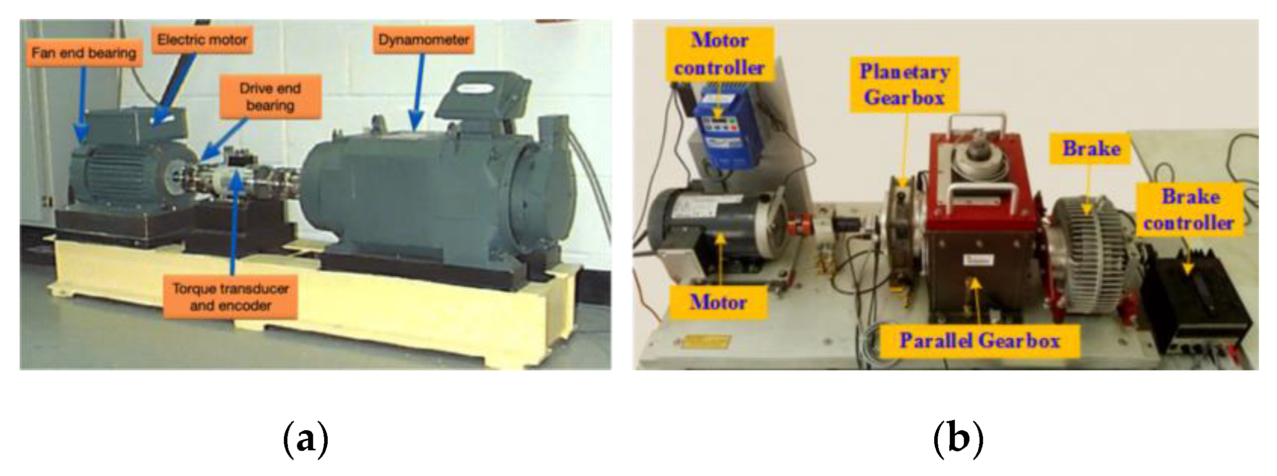
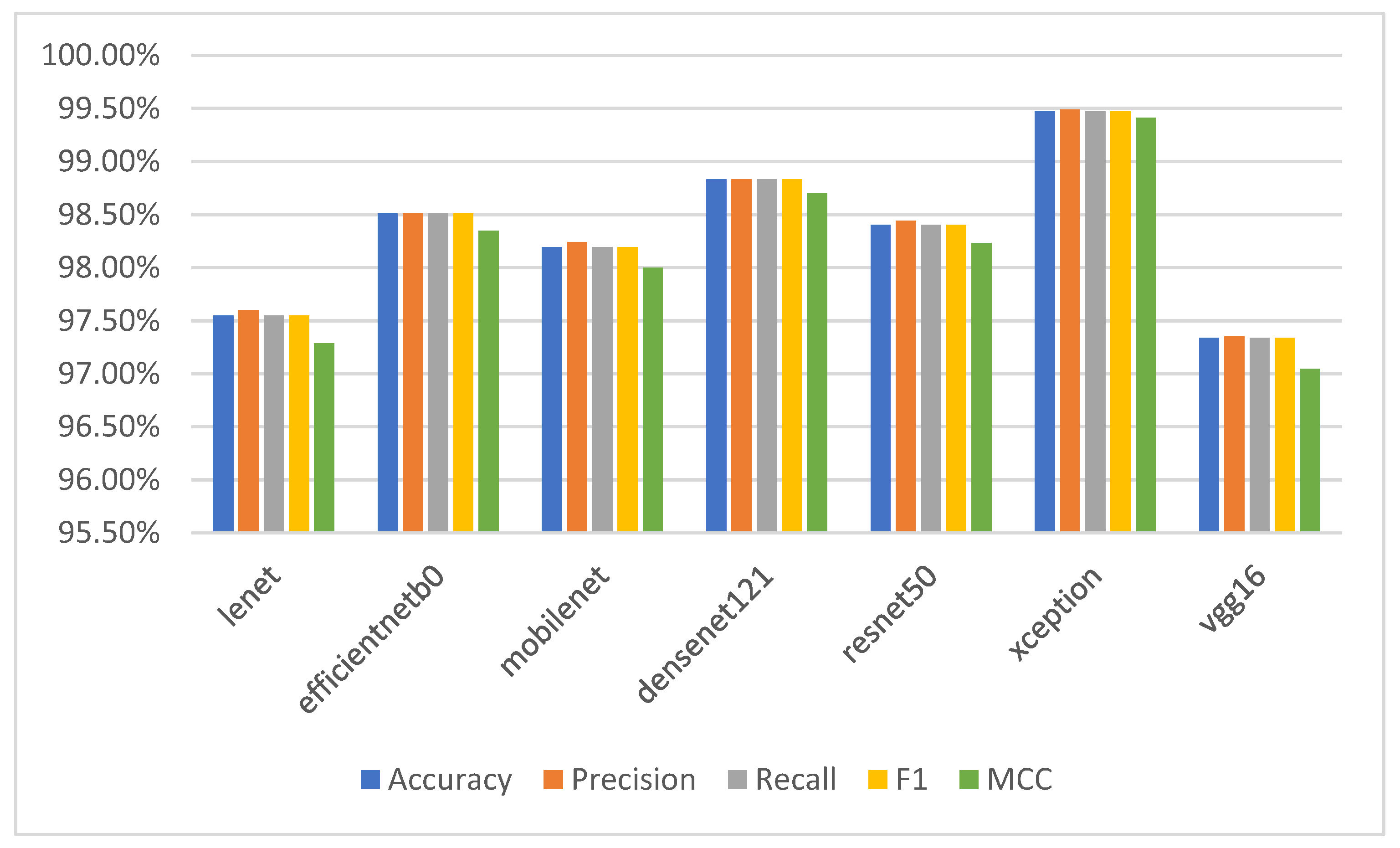
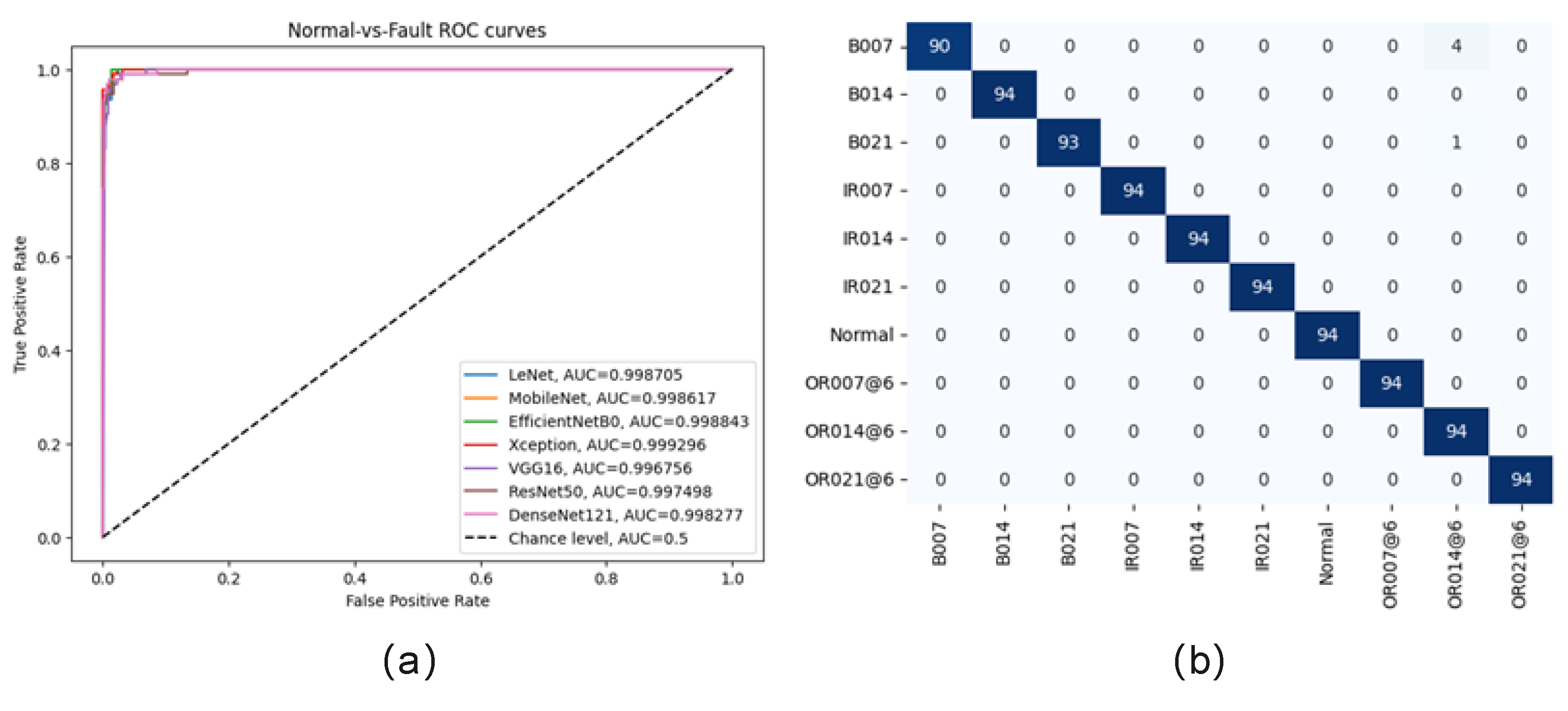
4.2. Case 1—CWRU Dataset (Uniaxial Signals)

In the first case, the bearing dataset collected by the Case Western Reserve University Bearing Data Center on a bearing test rig was utilised for framework validation with uniaxial signals [35]. The vibration signals in the experiment were collected from the uniaxial accelerometers on the drive end of the motor under one hp at the sampling frequency of 48 kHz. Different faulty bearings were introduced with fault diameters of 0.007, 0.014, and 0.021 inches on the rolling element, the inner raceway, and the outer raceway, respectively. Therefore, there are nine fault categories plus a normal baseline, i.e., ten kinds of bearing health states. The experiment aims to automatically recognise each fault category and select the most appropriate neural network for deployment through the proposed IFD framework.

Firstly, the uniaxial acceleration signals for each bearing health condition were separated into segments with the size of 1024 because the 32 × 32 pseudo-images can be utilised for most built-in APIs of classical CNN architectures directly in tf.keras. The segments were split randomly into the training, validation, and test sets according to 60%:20%:20%, i.e., 2820, 940, and 940 segments, respectively. Z-score standardisation was employed on the training set, and the fitted scaler transforms the test set. The segments were reshaped to single-channel matrices and duplicated into triple-channel pseudo-images through the pipeline in Figure 4. Subsequently, the pseudo-images were provided to the integrated CNN architectures as input for training and evaluation. Here, the pseudo-images were resized to 75 × 75 through nearest-neighbour interpolation when necessary to meet the input shape requirements of some CNN architectures, such as Xception. A fixed training configuration was employed in the experiment to test the framework availability for neural network selection, as shown in

Table 3. Training configuration.

Input Shape	Split	Epochs	Optimiser	Batch Size	Learning Rate
32 × 32 × 3 or 75 × 75 × 3	60%:20%:20%	1000	Adam	128	0.001

. Automatic hyperparameter optimisation can be further integrated in future work. The training loss and test accuracy are shown in Figure 8.

The checkpoint with the highest validation accuracy during training is saved as the best model for each CNN architecture. Their test performance can be seen in Figure 9, including accuracy, precision, recall, F1 score, and normal-vs-fault AUC. As can be seen, the Xception model with resized pseudo-images (75 × 75 × 3) as input has the best performance, and its confusion matrix is shown in Figure 10. The FLOPs, parameters, and average FPS (within 100 times) are shown in

Table 4. The CWRU model FLOPs, parameters, and FPS.

Models	LeNet	EfficientNetB0	Mobile-Net	Densnet-121	ResNet50	Xception	VGG16
FLOPs	6.58 × 105	8.66 × 106	1.16 × 107	5.79 × 107	7.89 × 107	5.62 × 108	3.32 × 108
Params	6.16 × 104	4.06 × 106	3.23 × 106	7.05 × 106	2.36 × 107	2.09 × 107	3.36 × 107
FPS	5449	2374	4058	1464	2463	1128	2760

. After conversion through TFLiteConverter [36], the derived lightweight Xception model can be deployed on an edge device, i.e., Raspberry Pi 4 (4GB) here, to satisfy the requirement for a practical application. It demonstrates that the proposed framework can achieve the model training, evaluation, and selection for IFD with the time-series signals from a uniaxial sensor by leveraging the popular built-in and self-defined CNN architectures based on AutoML, i.e., AutoML-CNN.

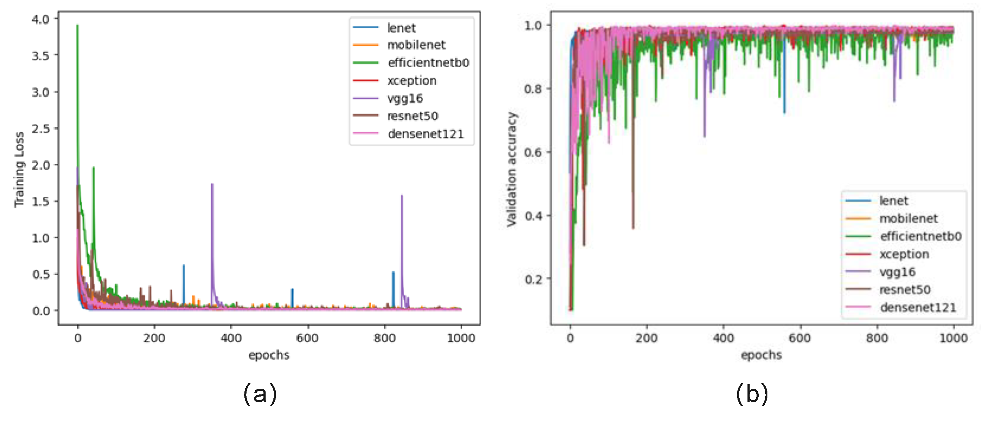
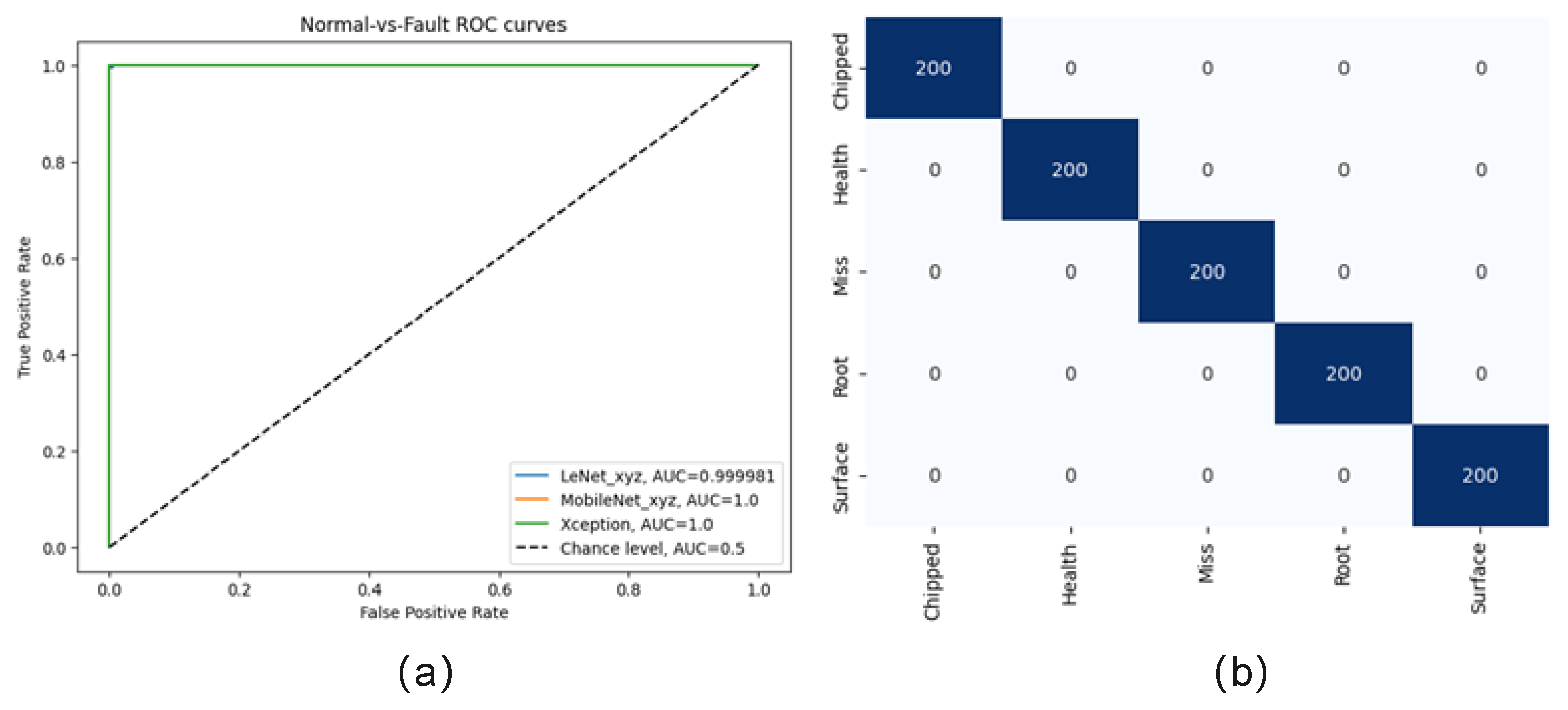
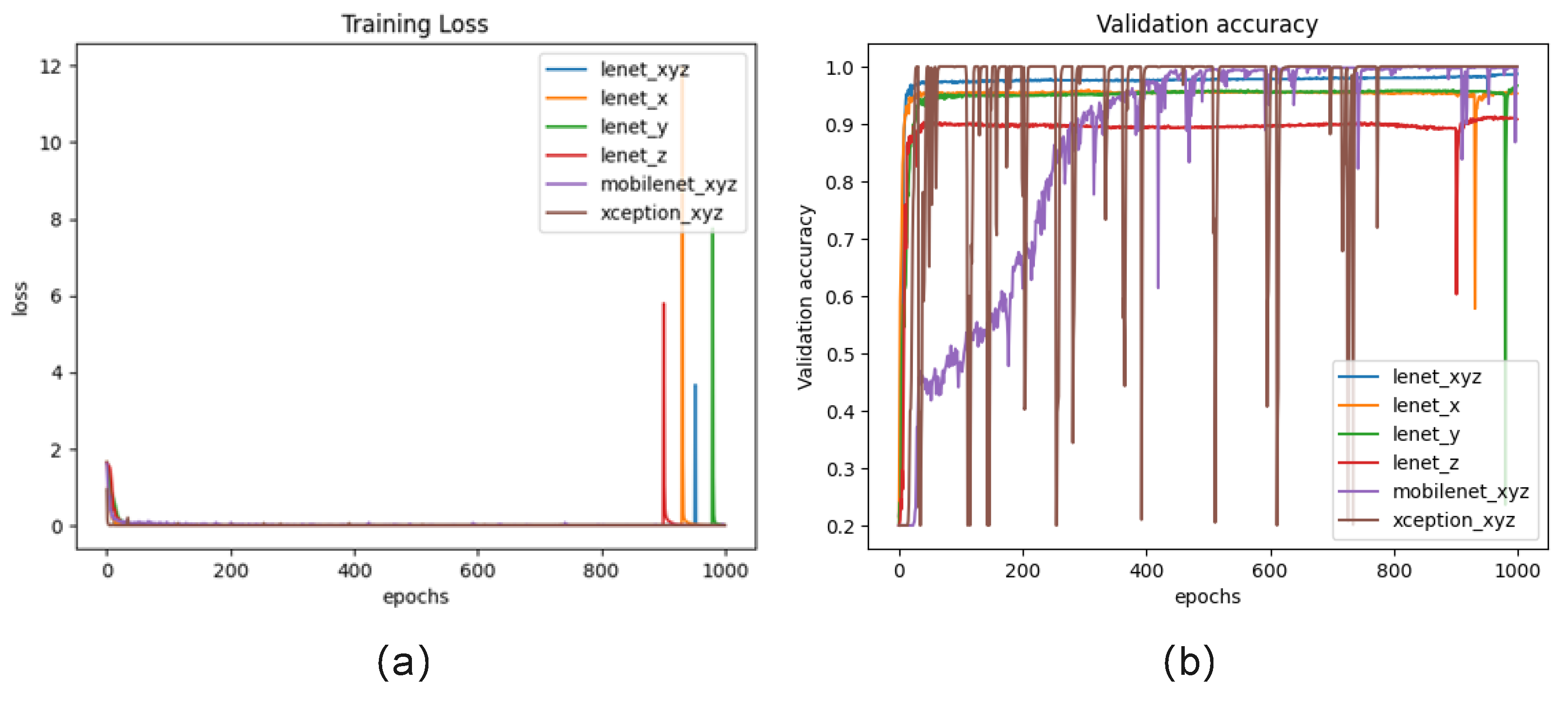
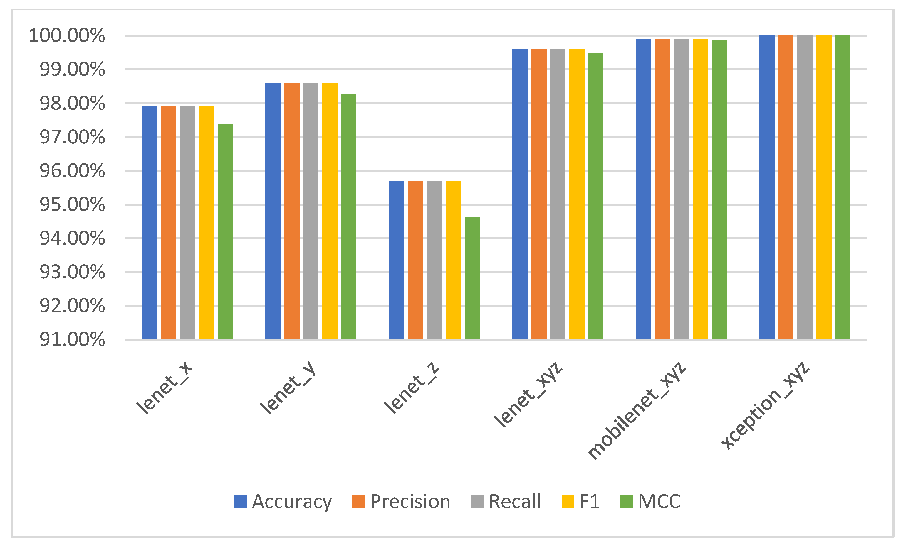
4.3. Case 2—SEU Dataset (Triaxial Signals)

In the second case, the gearbox dataset collected on the DDS (Drivetrain Dynamic Simulator) test rig of Southeast University was utilised for framework validation with triaxial signals. The planetary vibration data on triple axes (i.e., x, y, z) under the load configuration 30-2 was adopted for the experiment. There are four gear faults, including chipped tooth, missing tooth, root fault, surface fault, plus health working state, i.e., five kinds of gear health states. The experiment aims to automatically recognise each fault category and select the most appropriate neural network for deployment through the proposed IFD framework.

Initially, the planetary vibration signals for each axis were separated into segments with a size of 1024. Then, the segments were split randomly into the training, validation, and test sets under 60%:20%:20%, i.e., 3100, 1000, and 1000 segments, respectively. Z-score standardisation was employed on the training set, and the fitted scaler transformed the test set. Moreover, the segments were reconstructed into three-channel pseudo-images by stacking the single-channel image from each axis to achieve triaxial data fusion. Subsequently, the pseudo-images wer provided to the integrated CNN architectures as input for training and evaluation. Here, the pseudo-images were resized to 75 × 75 through nearest-neighbour interpolation to meet the input shape requirements of some CNN architectures, such as Xception, when necessary. Like case 1, a fixed training configuration was employed in the experiment, as shown in Table 3. The training loss and test accuracy are shown in Figure 11, where lenet_x, lenet_y, and lenet_z denote the LeNet-5 performance based on the data on a single axis. In contrast, lenet_xyz, mobile_xyz, and xception_xyz represent the model performance based on the triaxial data through the proposed image-like data fusion.

The test performance of each model, including accuracy, precision, recall, F1 score, and normal-vs-fault AUC, is shown in Figure 12, where x, y, z, and xyz denote the models with single- or triaxial signals. As can be seen, the model with the triaxial signals through the proposed image-like data fusion can achieve better performance than the model with the uniaxial signals, i.e., lenet_xyz performs better than lenet_x, lenet_y, and lenet_z. The Xception model with resized pseudo-images (75 × 75 × 3) as input has the best performance, and its confusion matrix is shown in Figure 13. The FLOPs, parameters, and average FPS (within 100 times) are shown in

Table 5. SEU model FLOPs and parameters.

Models	LeNet_x	LeNet_y	LeNet_z	LeNet_xyz	Mobile-Net_xyz	Xception_xyz
FLOPs	6.58 × 105	8.66 × 106	6.58 × 105	6.58 × 105	6.58 × 105	5.62 × 108
Params	6.16 × 104	4.06 × 106	6.16 × 104	6.16 × 104	6.16 × 104	2.09 × 107
FPS	5778	5585	5726	6003	3493	1161

. After conversion through the TFLiteConverter [36], the derived lightweight Xception model can be deployed on Raspberry Pi for practical applications. This demonstrates that data fusion and model training for IFD with the triaxial signals can be achieved through the proposed framework by leveraging AutoML-CNN and the proposed image-like data fusion.

5. Discussion and Conclusions

This work proposes an efficient and unified framework by leveraging AutoML and image-like data fusion for IFD with time-series signals from uniaxial or triaxial sensors. The popular built-in and self-defined DL architectures can be easily integrated into the framework to select the most suitable IFD model for different datasets or scenarios. Their training can be carried out consecutively or parallelly, and the evaluation can be taken automatically by comparing the model performance on the test set according to different metrics.. In the proposed spatial reconstruction method, the time-series data from a uniaxial sensor can be reshaped into a 2D matrix after normalisation and then duplicated into a three-channel pseudo-image. Similarly, the data from a triaxial sensor can be reconstructed into a three-channel pseudo-image by stacking the single-channel image from each axis, thereby achieving data fusion.

The proposed IFD framework and the data fusion method were validated via two case studies based on uniaxial and triaxial vibration signals from the CWRU and SEU datasets, respectively. The experiments demonstrate that it can automatically achieve model training and evaluation through the proposed IFD framework, thereby enhancing the development efficiency for practical applications. Moreover, the fused triaxial time-series data through the proposed image-like data fusion method can improve the model performance effectively. Moreover, the recommended DL model can be easily deployed on a cloud server or an edge device (such as Raspberry Pi) via tinyML for inference to satisfy the requirement for practical applications, such as in a DT manufacturing system, which requires timely and resilient decision-making, even under communication-constraint circumstances.

Although the proposed framework can benefit practical IFD application by leveraging AutoML and image-like data fusion, it still has some limitations. Firstly, the proposed data-level fusion method is only suitable for the signals from a single triaxial sensor or no more than three uniaxial sensors at the same sampling frequency. Hence, fusion methods for heterogeneous data from multiple sensors (more than three) with different sampling frequencies are required for future research. Secondly, as there is a trade-off between neural network performance and computing complexity, a more in-depth study for model recommendation considering practical scenarios, such as device computing capability, storage, and power, is also necessary for future work.

References

1. Peres, R.S.; Jia, X.; Lee, J.; Sun, K.; Colombo, A.W.; Barata, J. Industrial Artificial Intelligence in Industry 4.0-Systematic Review, Challenges and Outlook. IEEE Access 2020, 8, 220121–220139. [Google Scholar] [CrossRef]
2. Zhao, Z.; Zhang, Q.; Yu, X.; Sun, C.; Wang, S.; Yan, R.; Chen, X. Applications of Unsupervised Deep Transfer Learning to Intelligent Fault Diagnosis: A Survey and Comparative Study. IEEE Trans. Instrum. Meas. 2021, 70, 1–28. [Google Scholar] [CrossRef]
3. Tang, S.; Yuan, S.; Zhu, Y. Deep learning-based intelligent fault diagnosis methods toward rotating machinery. IEEE Access 2020, 8, 9335–9346. [Google Scholar] [CrossRef]
4. Zhang, T.; Chen, J.; Li, F.; Zhang, K.; Lv, H.; He, S.; Xu, E. Intelligent fault diagnosis of machines with small & imbalanced data: A state-of-the-art review and possible extensions. ISA Trans. 2022, 119, 152–171. [Google Scholar] [CrossRef]
5. Qiu, J.; Ran, J.; Tang, M.; Yu, F.; Zhang, Q. Fault Diagnosis of Train Wheelset Bearing Roadside Acoustics Considering Sparse Operation with GA-RBF. Machines 2023, 11, 765. [Google Scholar] [CrossRef]
6. Liu, Y.; Zhou, B.S.X.; Gao, Y.; Chen, T. An Adaptive Torque Observer Based on Fuzzy Inference for Flexible Joint Application. Machines 2023, 11, 794. [Google Scholar] [CrossRef]
7. Lei, Y.; Yang, B.; Jiang, X.; Jia, F.; Li, N.; Nandi, A.K. Applications of machine learning to machine fault diagnosis: A review and roadmap. Mech. Syst. Signal Process. 2020, 138, 106587. [Google Scholar] [CrossRef]
8. Pandya, D.H.; Upadhyay, S.H.; Harsha, S.P. Fault diagnosis of rolling element bearing with intrinsic mode function of acoustic emission data using APF-KNN. Expert Syst. Appl. 2013, 40, 4137–4145. [Google Scholar] [CrossRef]
9. Wang, J.; Liu, S.; Gao, R.X.; Yan, R. Current envelope analysis for defect identification and diagnosis in induction motors. J. Manuf. Syst. 2012, 31, 380–387. [Google Scholar] [CrossRef]
10. Jiang, X.; Li, S.; Wang, Y. A novel method for self-adaptive feature extraction using scaling crossover characteristics of signals and combining with LS-SVM for multi-fault diagnosis of gearbox. J. Vibroeng. 2015, 17, 1861–1878. [Google Scholar]
11. Praveenkumar, T.; Sabhrish, B.; Saimurugan, M.; Ramachandran, K.I. Pattern recognition based on-line vibration monitoring system for fault diagnosis of automobile gearbox. Measurement 2018, 114, 233–242. [Google Scholar] [CrossRef]
12. Wang, Z.; Zhang, Q.; Xiong, J.; Xiao, M.; Sun, G.; He, J. Fault Diagnosis of a Rolling Bearing Using Wavelet Packet Denoising and Random Forests. IEEE Sens. J. 2017, 17, 5581–5588. [Google Scholar] [CrossRef]
13. Liu, H.; Li, L.; Ma, J. Rolling Bearing Fault Diagnosis Based on STFT-Deep Learning and Sound Signals. Shock. Vib. 2016, 2016, 6127479. [Google Scholar] [CrossRef]
14. Lu, C.; Wang, Z.Y.; Qin, W.L.; Ma, J. Fault diagnosis of rotary machinery components using a stacked denoising autoencoder-based health state identification. Signal Process. 2017, 130, 377–388. [Google Scholar] [CrossRef]
15. Qiu, S.; Cui, X.; Ping, Z.; Shan, N.; Li, Z.; Bao, X.; Xu, X. Deep Learning Techniques in Intelligent Fault Diagnosis and Prognosis for Industrial Systems: A Review. Sensors 2023, 23, 1305. [Google Scholar] [CrossRef]
16. Ling, J.; Liu, G.J.; Li, J.L.; Shen, X.C.; You, D.D. Fault prediction method for nuclear power machinery based on Bayesian PPCA recurrent neural network model. Nucl. Sci. Tech. 2020, 31, 75. [Google Scholar] [CrossRef]
17. Yuan, M.; Wu, Y.; Lin, L. Fault diagnosis and remaining useful life estimation of aero engine using LSTM neural network. In Proceedings of the AUS 2016—2016 IEEE/CSAA International Conference on Aircraft Utility Systems, Beijing, China, 10–12 October 2016; pp. 135–140. [Google Scholar] [CrossRef]
18. Neves, A.C.; González, I.; Karoumi, R.A.C.; González, I.; Karoumi, R. A combined model-free Artificial Neural Network-based method with clustering for novelty detection: The case study of the KW51 railway bridge. In IABSE Conference, Seoul 2020: Risk Intelligence of Infrastructures—Report; IABSE: Zurich, Switzerland, 2021; pp. 181–188. [Google Scholar] [CrossRef]
19. Neves, A.C.; González, I.; Leander, J.; Karoumi, R. Structural health monitoring of bridges: A model-free ANN-based approach to damage detection. J. Civ. Struct. Health Monit. 2017, 7, 689–702. [Google Scholar] [CrossRef]
20. Sajedi, S.O.; Liang, X. Vibration-based semantic damage segmentation for large-scale structural health monitoring. Comput.-Aided Civ. Infrastruct. Eng. 2020, 35, 579–596. [Google Scholar] [CrossRef]
21. Wu, X.; Peng, Z.; Ren, J.; Cheng, C.; Zhang, W.; Wang, D. Rub-Impact Fault Diagnosis of Rotating Machin-ery Based on 1-D Convolutional Neural Networks. IEEE Sens. J. 2020, 20, 8349–8363. [Google Scholar] [CrossRef]
22. Sony, S.; Gamage, S.; Sadhu, A.; Samarabandu, J. Multiclass damage identification in a full-scale bridge using optimally tuned one-dimensional convolutional neural network. J. Comput. Civ. Eng. 2022, 36, 4021035. [Google Scholar] [CrossRef]
23. Sharma, S.; Sen, S. One-dimensional convolutional neural network-based damage detection in structural joints. J. Civ. Struct. Health Monit. 2020, 10, 1057–1072. [Google Scholar] [CrossRef]
24. Zhang, Y.; Miyamori, Y.; Mikami, S.; Saito, T. Vibration-based structural state identification by a 1-dimensional convolutional neural network. Comput.-Aided Civ. Infrastruct. Eng. 2019, 34, 822–839. [Google Scholar] [CrossRef]
25. Fahim, S.R.; Sarker, S.K.; Muyeen, S.M.; Sheikh, M.R.I.; Das, S.K.; Simoes, M. A Robust Self-Attentive Capsule Network for Fault Diagnosis of Series-Compensated Transmission Line. IEEE Trans. Power Deliv. 2021, 36, 3846–3857. [Google Scholar] [CrossRef]
26. Jiang, J.; Bie, Y.; Li, J.; Yang, X.; Ma, G.; Lu, Y.; Zhang, C. Fault diagnosis of the bushing infrared images based on mask R-CNN and improved PCNN joint algorithm. High Volt. 2021, 6, 116–124. [Google Scholar] [CrossRef]
27. Xia, M.; Li, T.; Xu, L.; Liu, L.; De Silva, C.W. Fault Diagnosis for Rotating Machinery Using Multiple Sen-sors and Convolutional Neural Networks. IEEE/ASME Trans. Mechatron. 2018, 23, 101–110. [Google Scholar] [CrossRef]
28. Gou, L.; Li, H.; Zheng, H.; Li, H.; Pei, X. Aeroengine Control System Sensor Fault Diagnosis Based on CWT and CNN. Math. Probl. Eng. 2020, 2020, 5357146. [Google Scholar] [CrossRef]
29. Meng, S.; Kang, J.; Chi, K.; Die, X. Intelligent fault diagnosis of gearbox based on multiple syn-chrosqueezing S-transform and convolutional neural networks. Int. J. Perform. Eng. 2020, 16, 528–536. [Google Scholar] [CrossRef]
30. Hoang, D.T.; Kang, H.J. Rolling element bearing fault diagnosis using convolutional neural network and vibration image. Cogn. Syst. Res. 2019, 53, 42–50. [Google Scholar] [CrossRef]
31. Wang, S.; Xiang, J.; Zhong, Y.; Zhou, Y. Convolutional neural network-based hidden Markov models for rolling element bearing fault identification. Knowl.-Based Syst. 2018, 144, 65–76. [Google Scholar] [CrossRef]
32. Wan, L.; Chen, Y.; Li, H.; Li, C. Rolling-element bearing fault diagnosis using improved lenet-5 network. Sensors 2020, 20, 1693. [Google Scholar] [CrossRef]
33. Teng, S.; Chen, G.; Liu, Z.; Cheng, L.; Sun, X. Multi-sensor and decision-level fusion-based structural damage detection using a one-dimensional convolutional neural network. Sensors 2021, 21, 3950. [Google Scholar] [CrossRef]
34. Gao, Y.; Li, H.; Xiong, G.; Song, H. AIoT-informed digital twin communication for bridge maintenance. Autom. Constr. 2023, 150, 104835. [Google Scholar] [CrossRef]
35. Gong, W.; Chen, H.; Zhang, Z.; Zhang, M.; Wang, R.; Guan, C.; Wang, Q. A Novel Deep Learning Method for Intelligent Fault Diagnosis of Rotating Machinery Based on Improved CNN-SVM and Multichannel Data Fusion. Sensors 2019, 19, 1693. [Google Scholar] [CrossRef] [PubMed]
36. Automated Machine Learning—Wikipedia. Available online: https://en.wikipedia.org/wiki/Automated_machine_learning (accessed on 16 August 2023).
37. Li, L.; Jamieson, K.; DeSalvo, G.; Rostamizadeh, A.; Talwalkar, A. Hyperband: A novel bandit-based approach to hyperparameter optimisation. J. Mach. Learn. Res. 2018, 18, 1–52. [Google Scholar]
38. Wu, J.; Chen, X.Y.; Zhang, H.; Xiong, L.D.; Lei, H.; Deng, S.H. Hyperparameter optimisation for machine learning models based on Bayesian optimisation. J. Electron. Sci. Technol. 2019, 17, 26–40. [Google Scholar] [CrossRef]
39. Ozaki, Y.; Tanigaki, Y.; Watanabe, S.; Onishi, M. Multiobjective tree-structured parzen estimator for computationally expensive optimisation problems. In Proceedings of the GECCO 2020—2020 Genetic and Evolutionary Computation Conference, Cancún, Mexico, 8–12 July 2020; pp. 533–541. [Google Scholar] [CrossRef]
40. Li, A.; Spyra, A.; Perel, S.; Dalibard, V.; Jaderberg, M.; Gu, C.; Budden, D.; Harley, T.; Gupta, P. A generalised framework for population-based training. In Proceedings of the ACM SIGKDD International Conference on Knowledge Discovery and Data Mining, Anchorage, AK, USA, 4–8 August 2019; pp. 1791–1799. [Google Scholar] [CrossRef]
Figure 1. The IFD pipeline through traditional machine learning [7].
Machines 11 00932 g001
Figure 2. The IFD pipeline through deep learning [7].
Machines 11 00932 g002
Figure 3. Reconstruction from time series to a single-channel grayscale image [30].
Machines 11 00932 g003
Figure 4. Proposed three-channel pseudo-image reconstruction from time series.
Machines 11 00932 g004
Figure 5. Proposed AutoML procedures for IFD.
Machines 11 00932 g005
Figure 6. Proposed framework by leveraging AutoML-CNN and image-like data fusion.
Machines 11 00932 g006
Figure 7. CWRU bearing and SEU DDS test rigs for data acquisition: (a) CWRU bearing test rig and (b) SEU DDS test rig.
Machines 11 00932 g007
Figure 8. IFD experiment for uniaxial acceleration data via the framework: (a) training loss and (b) validation accuracy.
Machines 11 00932 g008
Figure 9. Test performance on the CWRU dataset through the proposed pipeline.
Machines 11 00932 g009
Figure 10. (a) AUC for each model on the CWRU dataset and (b) confusion matrix of Xception on the CWRU dataset.
Machines 11 00932 g010
Figure 11. IFD experiment for triaxial acceleration data via the framework: (a) training loss and (b) test accuracy.
Machines 11 00932 g011
Figure 12. Test performance on the SEU dataset through the proposed pipeline.
Machines 11 00932 g012
Figure 13. (a) AUC for each model on SEU; (b) confusion matrix of Xception on SEU.
Machines 11 00932 g013