
On-Board Random Vibration-Based Robust Detection of Railway Hollow Worn Wheels under Varying Traveling Speeds †

Stochastic Mechanical Systems & Automation (SMSA) Laboratory, Department of Mechanical Engineering & Aeronautics, University of Patras, 26504 Patras, Greece
*
Author to whom correspondence should be addressed.
†
This Paper is an extension of the conference paper: On the On–Board Random Vibration–Based Detection of Hollow Worn Wheels in Operating Railway Vehicles. In Proceedings of the European Workshop on Structural Health Monitoring (EWSHM). Rizzo, P., Milazzo, A., Eds., Cham, 2021, pp. 480–489.
Machines 2023, 11(10), 933; https://doi.org/10.3390/machines11100933
Submission received: 27 July 2023
/
Revised: 21 September 2023
/
Accepted: 25 September 2023
/
Published: 28 September 2023
(This article belongs to the Special Issue Vibration and Acoustic Analysis of Components and Machines)
Abstract
:The problem of the prompt detection of early-stage hollow worn wheels in railway vehicles via on-board random vibration measurements under normal operation and varying speeds is investigated. This is achieved based on two unsupervised statistical time series (STS) methods which are founded on a multiple-model (MM) framework for the representation of healthy vehicle dynamics. The unsupervised MM power spectral density (U-MM-PSD) method employs Welch-based PSD estimates for wheel wear detection and the unsupervised MM autoregressive (U-MM-AR) method for the parameter vectors of multiple AR models. Both methods are assessed via two case studies using thousands of test cases. The first case study includes Monte Carlo simulations using a SIMPACK-based detailed railway vehicle model, while the second is based on field tests with an Athens Metro train. Wheel wear detection is pursued using lateral or vertical vibration signals from the bogie or the carbody of a trailed vehicle traveling with three different speeds (60, 70, 80 km/h) using wheels under healthy conditions or with early stage hollow wear. Both methods exhibit remarkable performance with the U-MM-AR method to achieve the best overall results, reaching correct detection rates of even 100% with false alarm rates below based on a single accelerometer either on the carbody or bogie.
1. Introduction
The good performance of railway vehicle wheels is an essential requirement for ensuring that a railway network is kept highly reliable and safe. The current wheel preventive maintenance schemes are susceptible to unplanned maintenance tasks, which lead to operational bottlenecks and increased cost due to the need for non-automated and time-consuming inspections, unscheduled disturbance to the timetable, and potentially untimely wheel replacement [1]. Railway vehicle wheel efficiency is strongly connected with the wheel/rail geometric parameters [2], which must remain within standard nominal ranges. Deviations from these affect the wheel–rail contact forces, which constitute the main dynamic loading of a railway vehicle, and may lead to passenger discomfort, damage in the neighboring rolling stock, degradation of the track infrastructure, or, in the worst case, to derailment [3].
Wheel defects may be classified into four major categories [4]: (i) defects on the wheel surface, such as wheel flats, spalling and shelling [5,6,7,8,9]; (ii) defects in the wheel profile (hollow worn wheels, flange wear, etc.); (iii) polygonization, including corrugation, wheels eccentricity, out of roundness (OOR) and so on [5,10,11]; and (iv) defects in the wheel subsurface, such as cracks, hardening and residual stresses [12,13,14]. The formation and evolution of wheel defects may be attributed to various sources, such as the type of the railway route, the wheel–rail adhesion conditions, the axle load, the train speed profile, the rail profile, and the wheel/rail material variability, as well as the occurrence of unexpected incidents, like payload shifts or the sudden braking of the vehicle. The prompt detection of wheel defects is necessary in any train prognostic and health management system (PHM), which operates using evidence-based maintenance strategies and may eliminate the adverse effects of unplanned maintenance tasks [15]. To this end, on-board condition monitoring, which is based on data collection from the railway vehicle during its normal operation, enables the real-time monitoring of rolling stock and especially wheels using sensors for measurement of vibration signals [16], acoustic emission [17] or strains [18]. However, vibration sensors and related data acquisition units are most commonly used due to such advantages as their reasonable cost, relatively simple instrumentation, the need for a limited number of sensors, as well as the fact that vibration signals contain rich information about the dynamics of the considered system, the proper analysis of which may lead to effective wheel defect detection [19].
Hollow wear is the most common type of wheel defect in railway vehicles, as it occurs and evolves gradually during the vehicle’s normal operation with the increase in the traveling distance, causing a hollow to the center of the wheel tread. Other reasons that may accelerate wheel hollow wear are the much softer wheel material compared to the material of the rail head, the contact of the brake shoe for trains with wheel–tread braking system, or the very small clearance between the wheel and track that allows for lateral motion of the wheelset on a narrow running surface on the wheel tread [5]. Hollow wear affects the wheel–rail contact forces and leads to higher wheel–rail interface stresses, rolling resistance, energy consumption and rail wear [20], implying that its monitoring and detection at an early stage is very important for all railway operations [3]. Additionally, severely hollow worn wheels may have detrimental effects on vehicle stability and curve mitigation that may lead to accidents [21,22].
Currently, the maintenance planning of hollow worn wheels relies mostly on frequent visual inspections, where measurements of the wheel profile are collected by skilled technicians using special tools with the vehicle being out of normal operation. If the wheel profile shape parameters are within specific standard limits, the vehicle continues its normal operation; otherwise, its wheels are reprofiled [23]. A standard measurement is the depth of the hollow to the center of the wheel tread, which is not allowed to be over ∼3 mm [22,23].
Based on the results of recent studies [24,25,26,27], it is evident that the effects of hollow worn wheels on the dynamics of a vehicle are detectable via on-board vibration measurements. This fact constitutes the motivation for the development of automated condition monitoring units for railway vehicle wheels that may be incorporated into a broader PHM system [1]. To this end, the on-board determination of wheel conicity and thus the monitoring of potentially hollow worn wheels is attempted in [28] through simulations with a simplified single wheelset model. The on-board condition monitoring of wheels conicity is also investigated in [16] via a supervised method, which is trained using vibration acceleration measurements from a railway vehicle with healthy and worn wheels under normal operation and constant speed. The natural frequency with the largest amplitude and the corresponding damping ratio are extracted from the vibration signals and used in a classification scheme for the detection of worn wheels. It is worth mentioning that the considered worn wheels cause significant increase to the RMS of the bogie frame lateral acceleration, implying that wheel wear is not at an early stage, while the method’s assessment is based on a limited number of test cases. Alternatively, data before and after wheel lathing from 52 Fiber Bragg Grating (FBG) strain sensors mounted in the bogie of a high speed train are used in [18] for the detection of abrupt changes through the determination of the Bayes factor. The method’s performance is assessed with the train running over specific track segments with constant speed before and after wheels reprofiling. It is noted that due to the significant changes to the measured (in time domain) stresses after wheels reprofiling, it is obvious that the considered wheels are characterized by significant defects before reprofiling, while temperature compensation is needed for the measured stresses.
The concept behind on-board methods is that wheel defects cause changes in the structural dynamics which are reflected on the measured signals (vibration, strain, and acoustic) and thus they may be detected via proper signal analysis. Yet, similar changes in the structural dynamics may be also caused by varying operating conditions (OCs), such as the traveling speed, payload and so on, which may be so significant as to partially or totally “mask” the changes due to wheel defects, especially if they are at an early stage [29], thus rendering proper detection highly challenging. The lack of robust methods capable of overcoming this difficulty, the fact that current methods can tackle detection for only significant and abrupt wheel wear characterized by clear effects on RMS values, and the relatively extensive instrumentation required constitute the current technology barriers, hindering the on-board robust, effective, and automated detection of early-stage hollow worn wheels on railway vehicles.
The goal of the present study is the introduction and assessment of a framework for the on-board detection of hollow worn railway vehicle wheels under normal operating conditions, addressing, for first time, the following issues:
- The unsupervised and robust detection of hollow worn wheels under different traveling speeds.
- The detection of hollow worn wheels at an early stage, before the standard hollow wear limit (∼3 mm) is reached and well before wear is evident on the RMS or related characteristics of acceleration signals on the vehicle bogie or carbody.
- The detection of hollow wheels using a single accelerometer on the vertical or lateral direction either on the vehicle bogie or carbody, thus keeping instrumentation at an absolutely minimal level.
The above are pursued via two statistical time series (STS) methods that operate based on the multiple model (MM) concept [30]: (i) the unsupervised MM power spectral density (U-MM-PSD) method, which is systematically postulated for the first time in this study and is founded on multiple Welch-based estimates [31] (pp. 186–187) of the PSD and a Euclidean distance metric; and (ii) the proper adaptation of the unsupervised MM autoregressive (U-MM-AR) method for the specific problem, which employs the parameter vectors of multiple AR models and a Kullback–Leibler divergence-based [32] distance metric.
These methods are fully data driven, signifying that they are not based on a complex physics-based model for the detection of wheel wear, which oftentimes needs assumptions and approximations for various unavailable vehicle parameters, as well as refinements via time-consuming optimization procedures using a significant number of experiments with the actual train and signals from many sensors. On the contrary, the above methods necessitate for their baseline learning phase a number of vibration signals from a single sensor on the vehicle carbody or bogie—collected while the train with healthy wheels are traveling on a tangent track at the speeds of interest—for the estimation of compact data-driven models, much simpler (fewer parameters) than a physics-based model, representing the partial vehicle dynamics under different speeds. In addition, the postulated methods operation in the inspection real-time phase for hollow worn wheel detection requires only a single vibration signal (from either the vehicle carbody or bogie) with the train traveling on a tangent track at a constant but not necessarily known speed under normal operation without braking, decelerating or accelerating. The small size of such data-driven models and the use of measurements from a single sensor lead to fast real-time decisions on the wheel condition, which do not overcome the few seconds.
Beyond the above-mentioned novelties, a unique performance assessment of the employed methods via a statistically reliable method based on two case studies and thousands of inspection phase test cases is undertaken. This is achieved through Monte Carlo simulations and vibration signals obtained from a detailed 42-DOF railway vehicle model developed in the SIMPACK commercial software [33] (Case Study A), as well as through field experiments with a third-generation Athens Metro vehicle (Case Study B). In both case studies, lateral and vertical vibration signals are acquired from sensors on the carbody and bogie frame of the considered vehicle, which operates normally under three different speeds (60, 70, and 80 km/h) on a tangent track, while the detection of hollow worn wheels at early stages corresponding to tread depths of ∼1 mm (Case Study A) and ∼2 mm (Case Study B), which do not affect the RMS values of the vibration signals, is investigated. Furthermore, various comparisons between the two methods, the considered sensor locations and the measurement directions are also considered using the true/false positive rates (TPRs/FPRs) that indicate the correct/false detection of the wheel condition (new/healthy or worn), respectively, and their pictorial representation via scatter type plots, receiver operating characteristic (ROC) curves [34,35] and area under the ROC (AUC) curve [35] bar plots. Partial and preliminary results based on specific test cases from the field experiments and measurements from only the vehicle’s bogie are presented in our recent conference paper [36].
The rest of the article is organized as follows: A precise problem statement is provided in Section 2. The description of Case Study A, including the Monte Carlo simulations, is presented in Section 3, while Case Study B with the field tests with the Athens Metro vehicle is described in Section 4. The multiple model-based methods for hollow worn wheel detection are presented in Section 5, while their performance assessment via the two case studies is shown in Section 6. A critical discussion on the results is presented in Section 7, and concluding remarks are finally summarized in Section 8.
2. Problem Statement
As mentioned above, the problem which is addressed in this study is the detection of early-stage hollow worn wheels in railway vehicles when the hollow wear is under a critical, user-selected (typically ) limit. To this end, the framework that is introduced in the present study operates in two basic phases, the baseline and the inspection phase as it is also described elaborately in Section 5.
- Baseline phase: Given a number n of random N-sample long lateral and/or vertical vibration response signals (presently accelerations)obtained from the railway vehicle running with distinct constant speeds during normal operation—excluding braking, deceleration or acceleration of the vehicle—over a tangent track with t designating normalization by the sampling period discrete time, the training of the framework is performed. These signals may be acquired from a sensor on the vehicle’s bogie or carbody (see Figure 1a,b) with the vehicle wheels considered under a healthy condition: hollow wear smaller than the selected critical limit.
- Inspection phase: Given a new random vibration signal from any of the above sensors’ location at any traveling speed with the vehicle wheels under an unknown condition (designated by the subscript u), the framework determines whether they are healthy or worn. This binary decision may be expressed via the following hypothesis testing using the distance metric D of either framework’s method (see details in Section 5) that should be under a limit
3. Case Study A: Monte Carlo Simulations with a SIMPACK Multibody Railway Vehicle Model
3.1. The Railway Vehicle Model
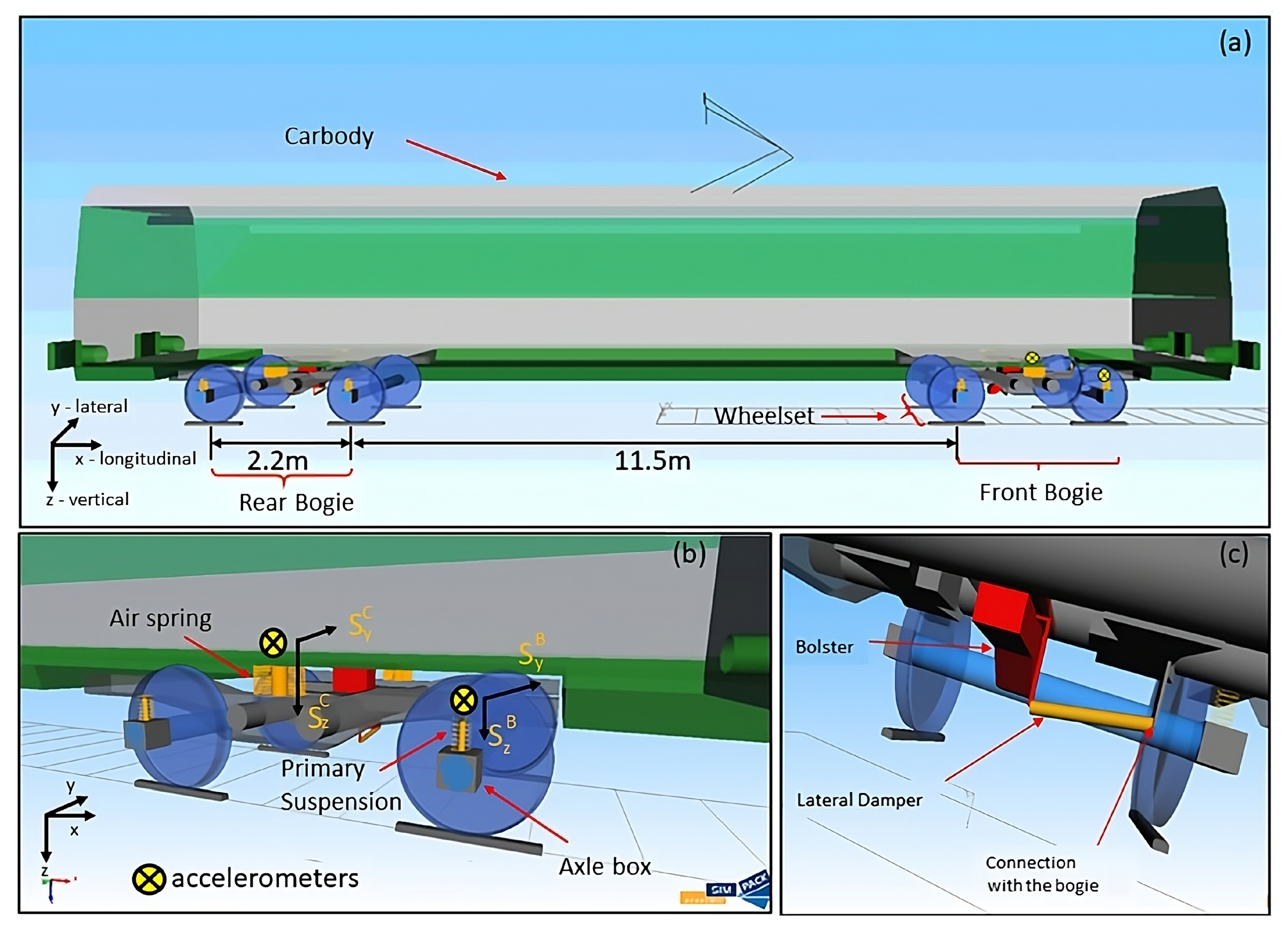
A detailed 42-DOF multibody model is developed in this case study for the dynamics representation of a trailed metro vehicle using the commercial software SIMPACK 2023 [33,37]. SIMPACK is commonly used in the railway industry and such models are generally accepted to offer sufficient representation of the train dynamics and used for various tasks in design, fault diagnosis, vehicle hunting, control and so on [38,39,40,41]. This model includes the vehicle’s carbody, two bogies, four wheelsets and eight axle boxes, all treated as rigid bodies (Figure 1a). The secondary suspension of the vehicle consists of a lateral damper and two air springs per bogie, and it connects the carbody with the bogie frame (Figure 1b). The lateral damper (Figure 1c) is typically simulated as a one-dimensional damper and the air spring as a linear spring with three-dimensional stiffness and damping. The primary suspension of the vehicle connects each axle box with the bogie frame via two rubber springs per axle box with each connection modeled as a single linear spring with three-dimensional stiffness and damping. The axle boxes are connected to the wheelset with kinematic constraints, which allow only pitch rotation simulating the axle bearing. The carbody, bogies and wheelsets allow all relative and absolute translative and rotational motions. More details about the parameters used in the vehicle’s model are shown in Appendix A.
According to the developed model, the vehicle runs in each simulation with a constant speed on a tangent track whose profile follows the UIC60 standard. The track irregularity, which is the main excitation to the moving vehicle, is modeled according to the ERRI B176 standard, including track corrugations, sleeper spacing, and rail manufacturing defects [42,43]. Based on this, low-amplitude vertical, lateral and cross-level irregularities are applied at wavelengths [0.08–25] m, [3–25] m, [3–25] m, respectively. It is noted that a different realization of track irregularity is applied to the vehicle in each simulation for the methods assessment to different track segments. Wheel–rail contact forces are calculated using the FASTSIM [44] algorithm, and model integration is achieved using the SODAST2 algorithm with a maximum timestep of s.
3.2. Hollow Worn Wheels and Monte Carlo Simulations
Two types of wheels are considered in each simulation, new or hollow worn wheels (Figure 2). The new wheel profile corresponds to brand new or freshly reprofiled wheels following the S1002 standard, while the worn profile is characterized by 1 mm hollow wear (maximum depth) to the wheel tread. It is worth stressing that this hollow wear is at an early stage and much smaller than the typical critical limit of ∼3 mm [22,23], which is also adopted by the Athens Metro company.
A total of 732 Monte Carlo simulations are performed at three different speeds of and 80 km/h as shown in Table 1. More specifically, a number of 122 simulations correspond to each considered speed and wheel condition, while vibration signals in the lateral and vertical direction are acquired from four accelerometers as shown in Figure 1b. Each accelerometer is designated as with p indicating its position (C for carbody or B for bogie) and d the measurement direction (lateral y or vertical z). Signals with a 50 s duration of steady-state vehicle running time are obtained in each simulation at a sampling frequency of 120 Hz. This frequency bandwidth is dominated by the track irregularity, which is negligible at higher frequencies [42,43]. All signals are normalized by subtracting their mean and dividing with their standard deviation. It is important to note that the assessment of the employed methods in Section 6 is performed using the signals from a single sensor per inspection test case.
3.3. Effects of the Vehicle Speed and Wheels Condition on the Vibration Signals and the Vehicle Dynamics
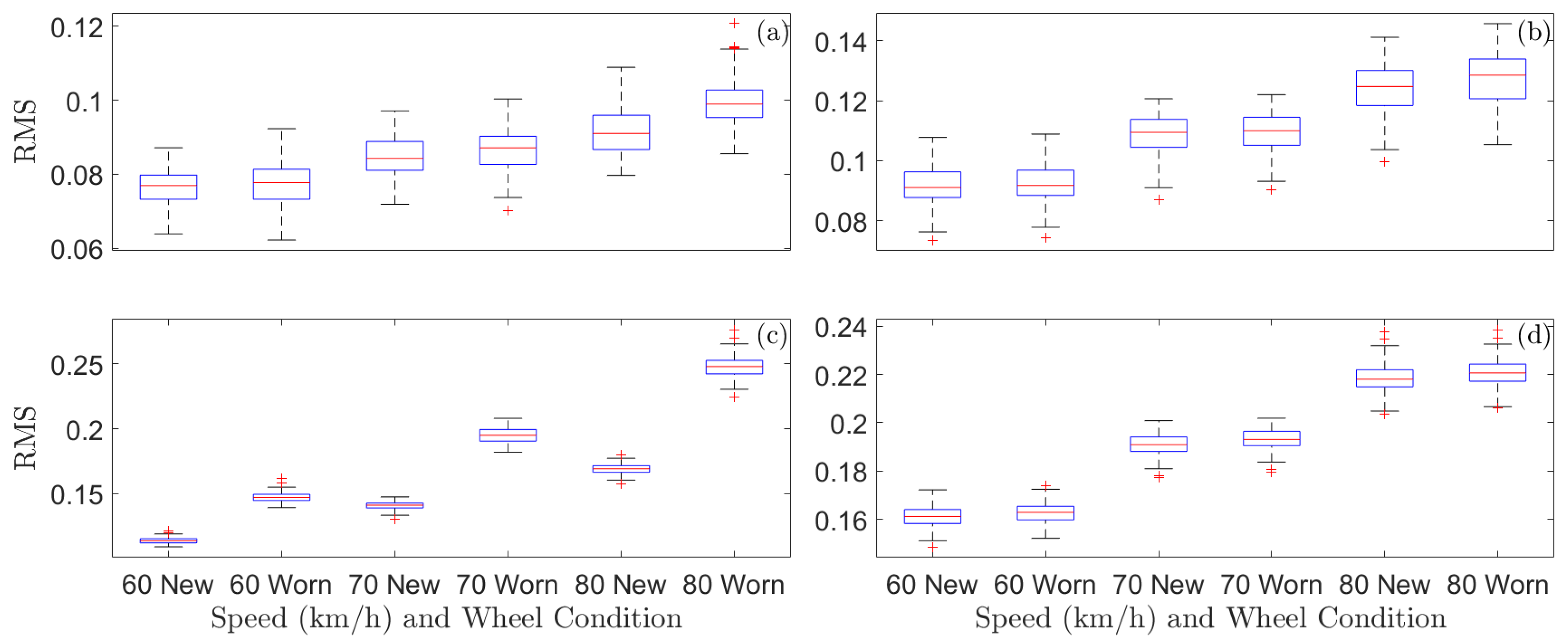
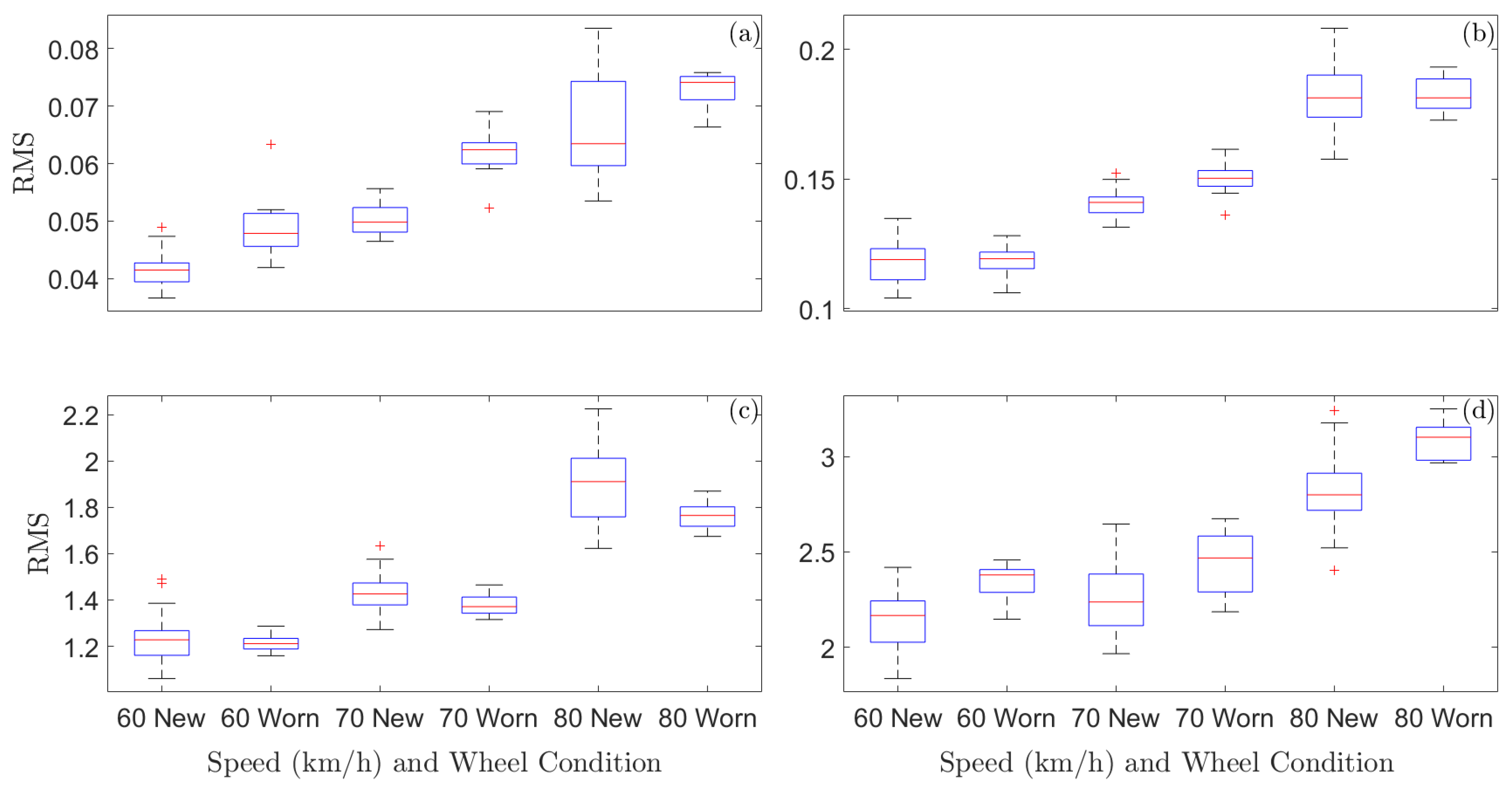
Indicative signals from all sensors and wheel conditions for a single speed are presented in Figure 3, while the RMS values from all signals per speed and wheel condition are depicted through typical box plots in Figure 4. According to the latter, it is clear that the RMS is significantly affected by the varying speed, and more specifically, it takes higher values with the increase in speed via any of the four sensors on the carbody or bogie. This, combined with the fact that the RMS corresponding to a low speed and hollow worn wheels is smaller than its counterpart at a higher speed and new (healthy) wheels, renders the RMS a non-robust feature for the detection of wheel wear under varying vehicle speeds. A further observation is that even for a single speed, the effects of the wheels hollow wear to the RMS are minor with no significant indication for wheel wear via any of the considered sensors with the exception of .
The above changes to the vibration signals from the varying vehicle speed imply, as expected, changes to the vehicle dynamics due to the spatial nature of the track irregularity [42,43], which is the main vehicle excitation, as well as the wheelbase-filtering effect [45]. The latter is caused by the repeated rail excitation to the wheelsets with time delays that depend on the vehicle speed and the length of the different wheelbases (distances between wheelsets) of the railway vehicle, which are shown in Figure 1a. In the following, the effects of the vehicle speed and worn wheels on the partial (related to sensor location) vehicle dynamics are explored via Welch-based PSD estimates. The estimation details for all PSDs are a window length of = 512 samples, overlap of = , and frequency resolution of = Hz.
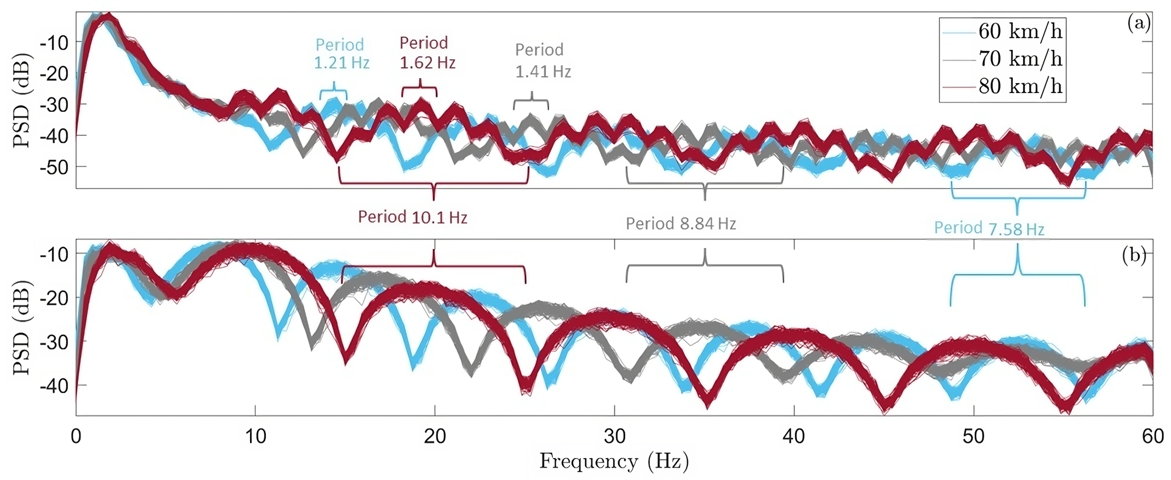
Indicative PSD envelopes, obtained from all measured signals via the and sensors, are shown in Figure 5, through which the effects of the different speeds on the lateral dynamics are evident. It is noted that the thickness of each envelope corresponding to a different speed is due to the railway vehicle running on a different track segment per simulation as previously mentioned. Similar effects are observed via the measurements of sensors and . Furthermore, some of the wheelbase-filtering frequencies are marked in Figure 5. For instance, the smaller frequencies (∼1 Hz) in Figure 5a correspond to the wheelbase-filtering effect due to the first–third and second–fourth pairs of wheelsets, which have the same wheelbase, while the higher frequencies, which also characterize the sharp valleys of Figure 5b, are due to the wheelsets of the bogies (see details in [45]).
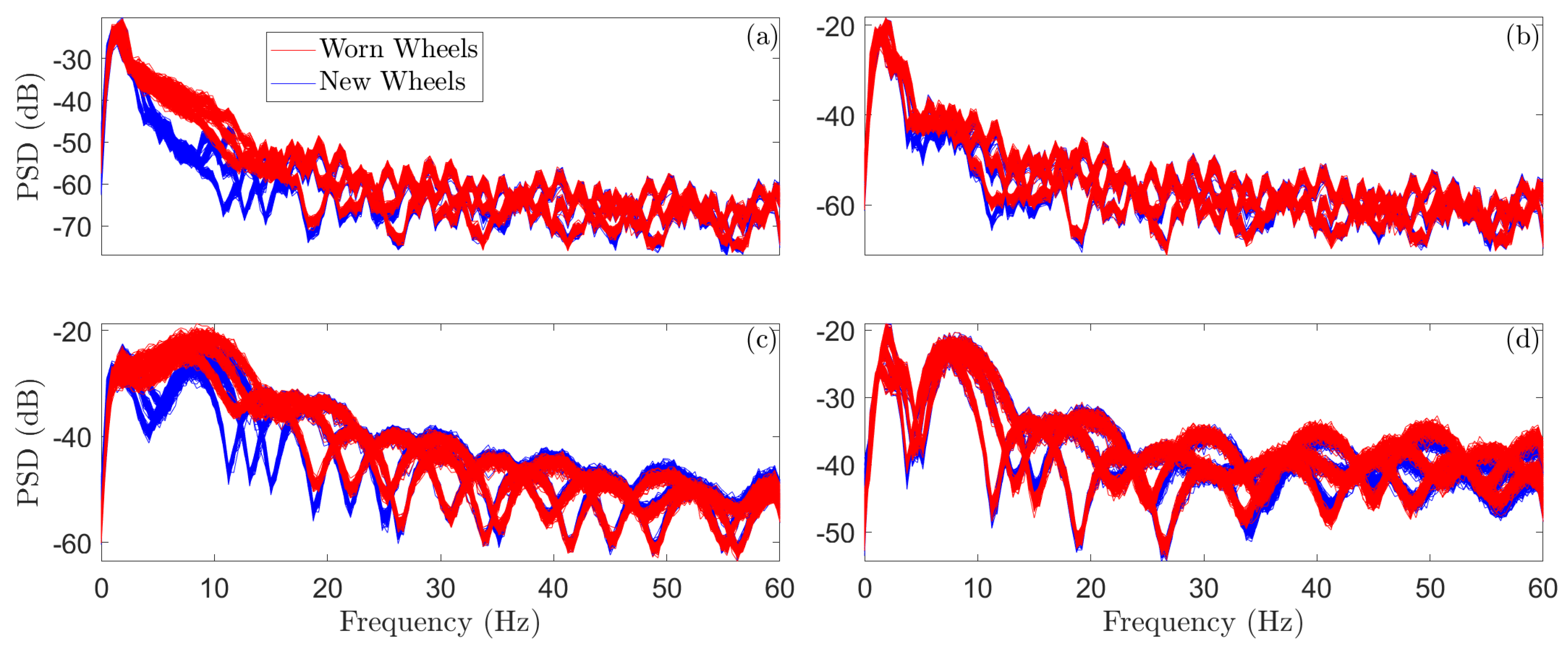
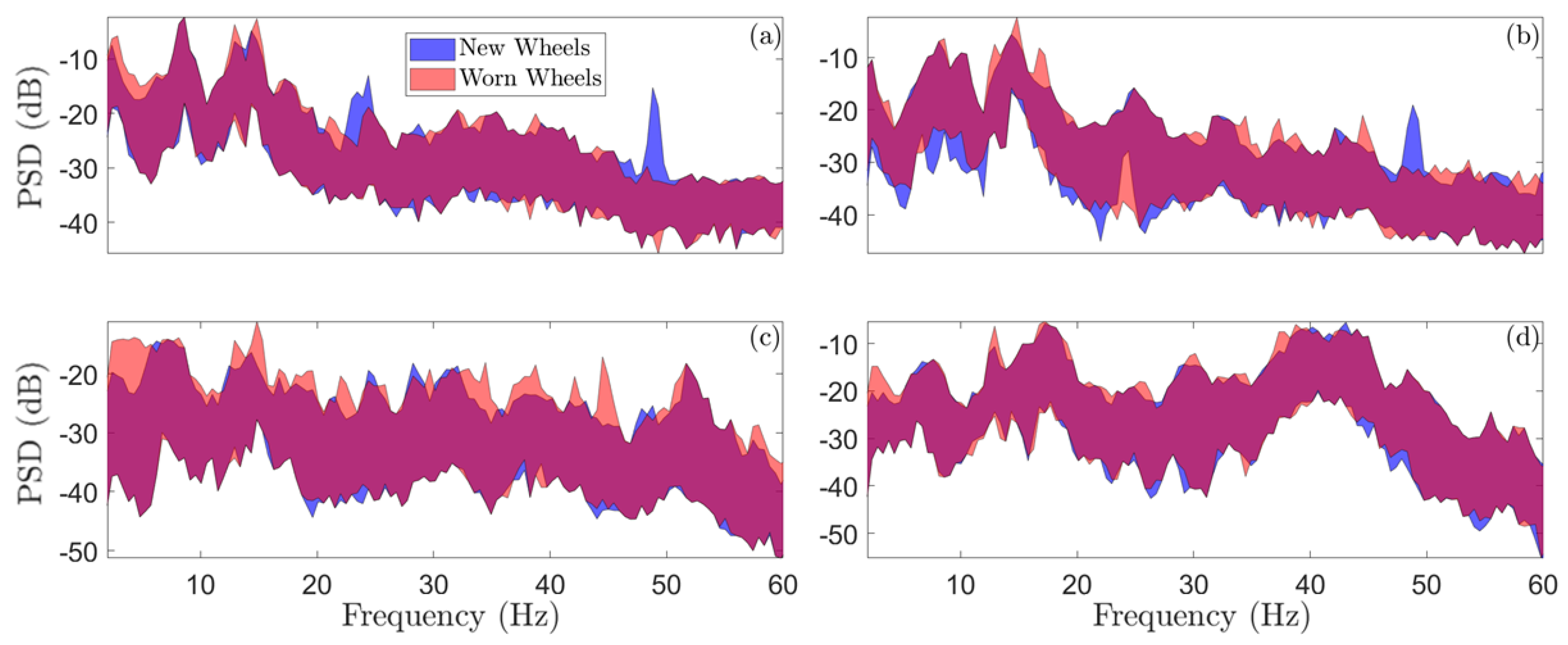
Similarly, indicative PSD envelopes corresponding to new and worn wheels and measurements from all sensors with vehicle speed equal to 60 km/h are shown in Figure 6. The effects of worn wheels are more noticeable in the lateral dynamics for both the carbody (Figure 6a) and bogie frame (Figure 6c), and especially in low frequencies up to 10 Hz. On the other hand, the vertical dynamics is significantly less affected by the considered early-stage wheel hollow wear according to Figure 6b,d. This is expected, as hollow worn wheels affect the lateral dynamics of a railway vehicle to a greater degree.
Finally, Figure 7 depicts the PSD envelopes based on all sensors and for all considered speeds and wheel conditions, from which it is confirmed that the vehicle lateral dynamics is more sensitive to hollow worn wheels, as well as that the effects of the varying speed on the dynamics may “mask” the effects of hollow worn wheels and set a highly challenging detection problem.
4. Case Study B: Field Tests with an Athens Metro Train
4.1. The Train and the Measurement Set-Up
The field tests are performed with a typical 3rd generation Athens Metro train, manufactured by Hyundai–Rotem–Hanwha. This is a 6-car train that consists of two motorcars with a driver cab, two motorcars without a driver cab and two trailing cars (Figure 8). The train is 106 m long and has a total tare weight of 182 tons. It is powered by 16 AC asynchronous motors of 175 kW each, with two motors per bogie and has a maximum operational speed of 80 km/h. The tested train first went into operation in 2014, covering approximately 80.000 km/year. Two uniaxial accelerometers are mounted at two different locations on the bogie frame of one of the two trailing cars (Figure 8) in order to measure vertical and lateral acceleration, while one triaxial accelerometer is additionally mounted in the carbody over the air spring as shown in Figure 8. The vertical and lateral vibration signals from all sensors are collected through a portable high-fidelity data acquisition PXI unit from National Instruments. For notational simplicity, the symbol is used for each employed sensor as in Case Study A, with d indicating the measurement direction and p the sensor position.
4.2. Operating Conditions and Random Vibrations Signals
Vibration measurements are collected from the trailing car before and after the wheel reprofiling. The wheel hollow wear was ∼2 mm before reprofiling, and as in Case Study A, the wheels are referred to as new or worn. Field tests are carried out with new and worn wheels on a tangent track under three different and constant speeds (60, 70, and 80 km/h ± 3 km/h) without passengers on board.
Random vibration measurements are acquired with a sampling frequency of Hz via , , , and (Figure 8) and high-pass filtered using a Chebyshev type II filter of order 18 and cut-off frequency Hz in order to eliminate noise effects at lower frequencies due to the employed accelerometer specifications. Signal segments affected by vehicle abrupt acceleration or deceleration, braking and rail crossings are removed, while the operational frequency bandwidth is selected as [0–60] Hz for direct comparisons with the previous case study. The vibration signals are normalized by subtraction of their mean and division with their standard deviation. Details on the acquired vertical and lateral signals are shown in Table 2.
4.3. Effects of the Vehicle Speed and Worn Wheels on the Vibration Signals and the Vehicle Dynamics
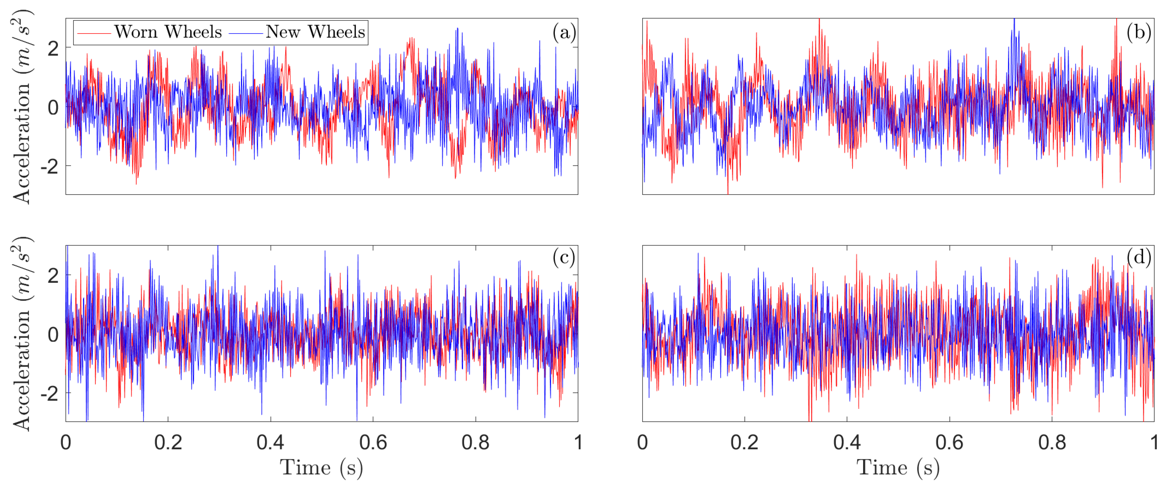
Indicative signal segments from the field tests via all considered sensors, with new and worn wheels, are shown in Figure 9. It is noted that all measurements were acquired from a typical Athens Metro train with potential slight fatigue to the wheels, suspensions and other mechanical parts that affect the amplitude of the acceleration measurements, and the train was traveling on a track that has been used by many trains and for several years, with the expectation of significantly more abrasive track irregularity than the one used in Case Study A. This non-ideal condition of the employed train and track is confirmed through the comparison of the acceleration signals of Figure 3 with the signals in Figure 9, with the max amplitude in the latter being significantly higher.
The RMS values of the vibration signals from all vehicle speeds and wheel conditions and from all sensors are, as in the previous case study, shown in Figure 10. The evidence that the RMS increases with the increase in the vehicle speed is confirmed. Yet, in this case study, there is no clear discrimination between new and worn wheels based on the RMS values and any sensor, even if a single speed is considered. This indicates that the RMS is a non-robust feature for worn wheel detection when delicate types of wheels wear, such as that to the hollow of the wheel tread, are investigated.
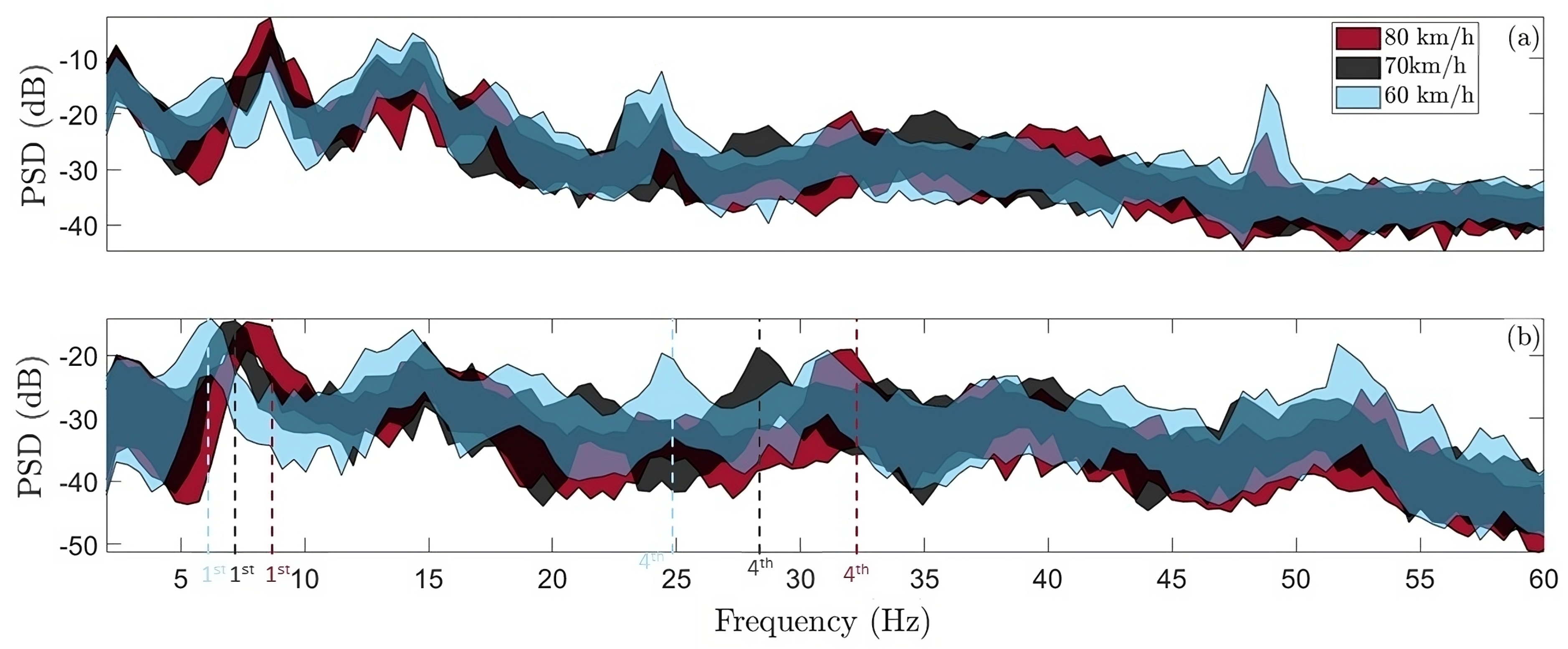
Figure 11 includes indicative envelopes of Welch–based PSD estimates (estimation details: Window length samples, overlap , frequency resolution Hz) using lateral vibration signals from the carbody and bogie for the three considered traveling speeds. As expected, the effects of the varying speed on the vehicle dynamics are evident at various frequencies of the PSD envelopes. It is worth noting that some of the running speed induced changes to the bogie PSD envelopes correspond to the wheels rotation frequency, that is Hz for speed of 60 km/h, Hz for speed of 70 km/h and Hz for speed of 80 km/h as shown in Figure 11b, and its 4th harmonic (, , Hz for 60, 70 and 80 km/h, respectively). Additionally, the wheelbase-filtering effect is not noticeable in this case study, as the obtained measurements include far more complex dynamics compared to Case Study A, due to vehicle excitation from various sources, other than track irregularity, such as the interaction among the wheelsets of the six vehicles, the motors in four vehicles of the train, air condition compressors, and so on.
Similarly, the effects of the worn wheels on the vehicle dynamics are shown in the PSD envelopes of Figure 12 for vehicle speed of 70 km/h. Based on this, it is again observed that the wheel hollow wear has more significant effects on the lateral dynamics (see Figure 12a,c), and especially on the bogie measurements. The red arrows in this figure indicate peaks of worn wheel frequencies that match wheel out-of-roundness (OOR) orders [10], which herein are observable up to the order of seven. These frequencies are harmonics of the fundamental wheel rotation frequency , with v designating vehicle speed and mm wheel diameter. When the train travels with 80 km/h, the seventh harmonic corresponds to Hz, indicating the appropriateness of the selected operational bandwidth up to 60 Hz. It is referred [46] that in metro vehicles, OOR may evolve along with wheel hollow wear [26].
Finally, the almost completely overlapped PSD envelopes in Figure 13 using signals from any sensor with new or worn wheels, indicate, as in the previous case study, the generally highly challenging problem of robust wheel wear detection under varying train speed that is investigated in this study. It should be stressed that the problem is severely aggravated when on-board measurements from actual trains are used, as these are significantly affected by various other factors as mentioned above.
5. The Wheel Wear Detection Methods
Two robust (with respect to the varying OCs) statistical time series (STS) methods are employed in the introduced framework for wheel wear detection, which operate based on the general concept of using multiple models (MMs) for the representation of system dynamics under various conditions [30]. The first method, abbreviated as U-MM-PSD, is unsupervised and is founded on multiple nonparametric representations (models), each one corresponding to the PSD obtained from vibration signals which are acquired under different OCs. The second unsupervised method, abbreviated as U-MM-AR [30], is alternatively based on multiple parametric autoregressive (AR) models for the dynamics representation. Both methods have a baseline (learning) phase, where their training is performed using vibration signals from the vehicle with healthy wheels under various speeds in the range of interest, and an inspection phase, where the wheel monitoring is performed in real time with the train under normal operation based exclusively on the measured vibration signals. The distinct steps of each method are presented in the following.
5.1. The U-MM-PSD Method
- Step 1:
- Multiple model representation (baseline phase). The MM representation of the railway vehicle dynamics is constructed in this step based on the n signals of the baseline phase (also see Section 2); the use of the same number of signals per speed is preferred. Thus, the MM representation in this method consists of n Welch-based [31] (pp. 186–187) PSD estimates. The obtained values of the PSD constitute the method’s feature vector—the complete or part of the measured frequency bandwidth may be used (the PSD in the 2–60 Hz frequency range is herein suggested for the detection of early-stage wheel hollow wear)—while the PSD estimate from a single (from the n) signal corresponds to a single model from the set of models that compose the MM representation.
- Step 2:
- Feature vector reduction (baseline phase). The reduction in the feature vector dimensionality is performed in this step in order to remove frequencies with high sensitivity to the varying OCs (presently, the vehicle’s speed). Thus, the PSD sample variance per frequency is obtained, and the frequencies are reordered in the feature vector from the one with the minimum variance to that with the maximum. The first k frequencies are retained in the feature vector, with k being user defined.
- Step 3:
- Inspection phase. Once a fresh vibration signal is obtained in real time from the vehicle with wheels of unknown condition, the objective in this step is to decide whether or not the current vehicle dynamics belongs to the MM representation . If it does, then the wheels are indicated as healthy, and otherwise as worn. To this end, a new PSD estimate, , is obtained based on the measurements of this phase (also see Section 2), and the method’s feature vector is formulated in order to include the PSD values of the frequencies selected to the previous step. Then, the following distance metricD is utilized for the decision making:with designating the Euclidean distance. The detection of worn wheels is then declared if and only if , with determined based on the values of the D metric in the baseline phase.
5.2. The U-MM-AR Method
- Step 1:
- Multiple model representation (baseline phase). As for the previous method, this step includes the construction of the MM representation of the railway vehicle dynamics based on the n signals of the baseline phase; the same number of signals per speed is also suggested for this method. Thus, the MM representation in this method consists of n AR models (each one estimated using a single vibration signal) of the form [30]with designating the model order, the j-th AR parameter, and the model residual that should be a white Gaussian zero-mean sequence with variance . stands for normally independently distributed with the indicated mean and variance. The method’s feature vector for worn wheels damage detection is the AR model parameter vector (bold-face upper-/lower-case symbols: matrix/column vector quantities; : matrix transposition) which is obtained along with its covariance for each AR model based on standard identification procedures [31] (pp. 318–320), using the ratio of the model residual sum of squares to signal sum of squares (RSS/SSS %), the Bayesian information criterion (BIC) and the samples per estimated parameter (SPP) for the model order selection.It is noted that once the parameters of the multiple AR models have been estimated, these may be considered surrogate models based on the fact that they may represent the vehicle partial (with respect to the employed sensor location) dynamics under different traveling speeds. Such a model may also provide predictions of the vehicle acceleration response at the sensor location using the time history of the measurements at that point.
- Step 2:
- Inspection phase. As for the previous method, once a fresh vibration signal is obtained in real time from the vehicle under unknown speed and wheel condition, a new AR model of the same order as those in with parameter vector is estimated, and a distance metric, such as that in Equation (1), is used for the detection of the worn wheels, with designating in this method the Kullback–Leibler divergence [32] between the models and :where is the trace and the determinant of the indicated matrix. As previously, if D exceeds a user-defined critical limit—which is set in the baseline phase based on signals from the vehicle with the healthy wheels—then the unknown wheels condition is declared as worn, and otherwise as healthy.
6. Performance Assessment of the Wheel Wear Detection Methods
6.1. Assessment Procedure
The performance assessment of both detection methods is based on an iterative “rotation” procedure of the set of signals, which are used in the baseline phase according to the S-fold cross validation [47] (p. 33). Based on this, the potential dependence of the methods learning, and thus their performance, on specific sets of signals is eliminated, ensuring statistically more reliable results. So, let there be h and f signals from new and worn wheels, respectively. From the h signals, a randomly selected set of b signals, equally distributed per speed (60, 70 and 80 km/h), is used for the methods’ Step 1 (also see Section 5) in the first iteration of the rotation procedure. The remaining signals from the vehicle with new wheels, say , and the f signals from the vehicle with worn wheels, that is , are considered as being originated from unknown health states and are used in the inspection phase for testing the methods’ performance. The procedure continues with a next rotation that begins with a different set of b signals. Once a number q of rotations that leads to an adequate number of aggregated inspection test cases are completed, the procedure stops. In this study, 3360 test cases for Case Study A (see Table 3) and 5600 for Case Study B (see Table 4) are deemed adequate for testing the methods’ performance.
The performance of the wheels wear detection methods is presented via receiver operating characteristic (ROC) curves, each presenting the true positive rate (TPR) (probability of correct wear detection), versus the false positive rate (FPR) (probability of false alarm) for varying decision thresholds [34]. In addition, scatter-type plots, including the methods’ distance metric D, are used.
6.2. Performance Assessment of the U-MM-PSD Method
- Case Study A. Welch-based PSD estimates are obtained using vibration signals (20 per speed) in Step 1 of the baseline phase for each rotation (also see Table 3) and for each of the considered sensors. All details about the method per employed sensor are shown in Table 5, while the method’s distance metric D plot and the corresponding ROC curves are illustrated in Figure 14 and Figure 15, respectively. Based on these, the method’s performance is characterized as follows.
Figure 14.
Case Study A—distance metric plot for the U-MM-PSD method based on sensors (a) , (b) , (c) , (d) (3360 inspection test cases).
Figure 14.
Case Study A—distance metric plot for the U-MM-PSD method based on sensors (a) , (b) , (c) , (d) (3360 inspection test cases).

Figure 15.
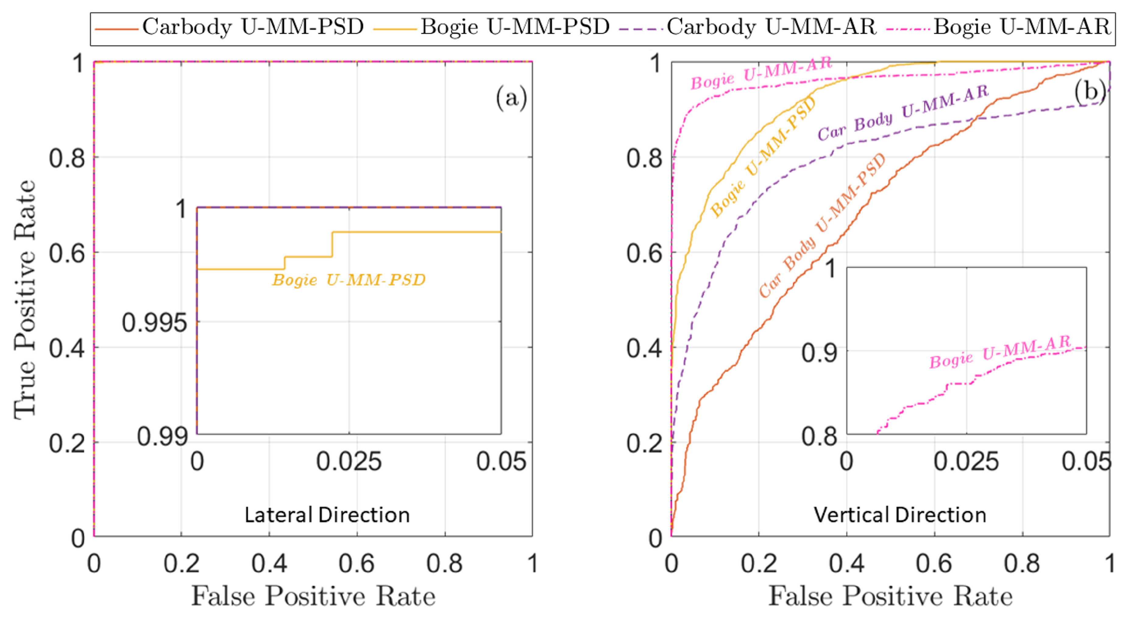
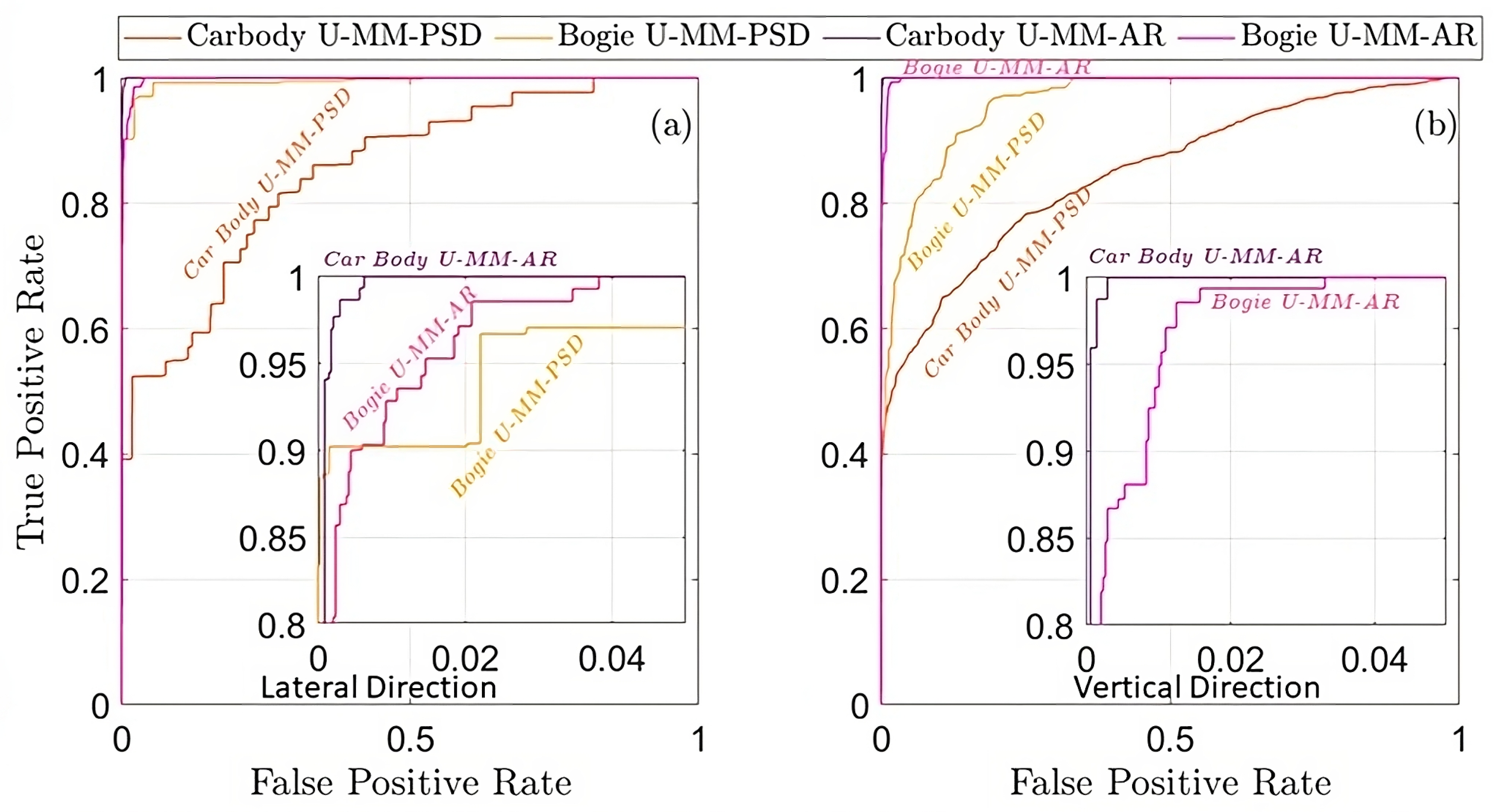
Case Study A—worn wheels detection performance assessment for the U-MM-PSD and U-MM-AR methods via ROC curves based on sensors (a) , , and (b) , (3360 inspection test cases).
Figure 15.
Case Study A—worn wheels detection performance assessment for the U-MM-PSD and U-MM-AR methods via ROC curves based on sensors (a) , , and (b) , (3360 inspection test cases).

Table 5.
Case Study A—details on the wheels wear detection methods.
| Method | Feature | Feature Vector Length Per Sensor | Distance Metric |
|---|---|---|---|
| U-MM-PSD * | PSD vector | Euclidean | |
| U-MM-AR ** | AR parameter vector | Kullback–Leibler |
* Welch-based estimation: segment length: 1024 samples, overlap: 90%, freq. resolution: Hz. ** RSS/SSS (%) = , BIC = −10.18/−9.03/−6.22/−5.07, SPP = .
According to the results of this case study, it is evident that the method’s performance is far better using lateral vibration measurements.
- Case Study B. As in the previous case study, the method is applied using vibration signals (20 per speed) from each of the considered sensors in the baseline phase and for each rotation (also see Table 4). The details of the method’s operation per employed sensor are shown in Table 6. The method’s distance metric D plots and the corresponding ROC curves are presented in Figure 16 and Figure 17, respectively. Based on these, the method’s performance is characterized as follows.
Figure 16.
Case Study B – distance metric plot for the U-MM-PSD method based on sensors (a) , (b) , (c) , (d) (5600 inspection test cases).
Figure 16.
Case Study B – distance metric plot for the U-MM-PSD method based on sensors (a) , (b) , (c) , (d) (5600 inspection test cases).

Figure 17.
Case Study B – worn wheel detection performance assessment for the U-MM-PSD and U-MM-AR methods via ROC curves based on sensors (a) , , and (b) , (5600 inspection test cases).
Figure 17.
Case Study B – worn wheel detection performance assessment for the U-MM-PSD and U-MM-AR methods via ROC curves based on sensors (a) , , and (b) , (5600 inspection test cases).

Table 6.
Case Study B—details on the wheel wear detection methods.
| Method | Feature | Feature Vector Length Per Sensor | Distance Metric |
|---|---|---|---|
| U-MM-PSD * | PSD vector | 113/4/117/42 | Euclidean |
| U-MM-AR ** | AR parameter vector | 140/150/110/90 | Kullback–Leibler |
* Welch-based estimation: segment length: 512 samples, overlap: 90%, freq. resolution: Hz. ** RSS/SSS (%) = , BIC = −8.96/−9.89/−9.25/−10.13, SPP = .
As in the previous case study, the results from the field tests indicate that measurements at the lateral direction and especially from the bogie frame may lead to remarkable detection of hollow worn wheels.
6.3. Performance Assessment of the U-MM-AR Method
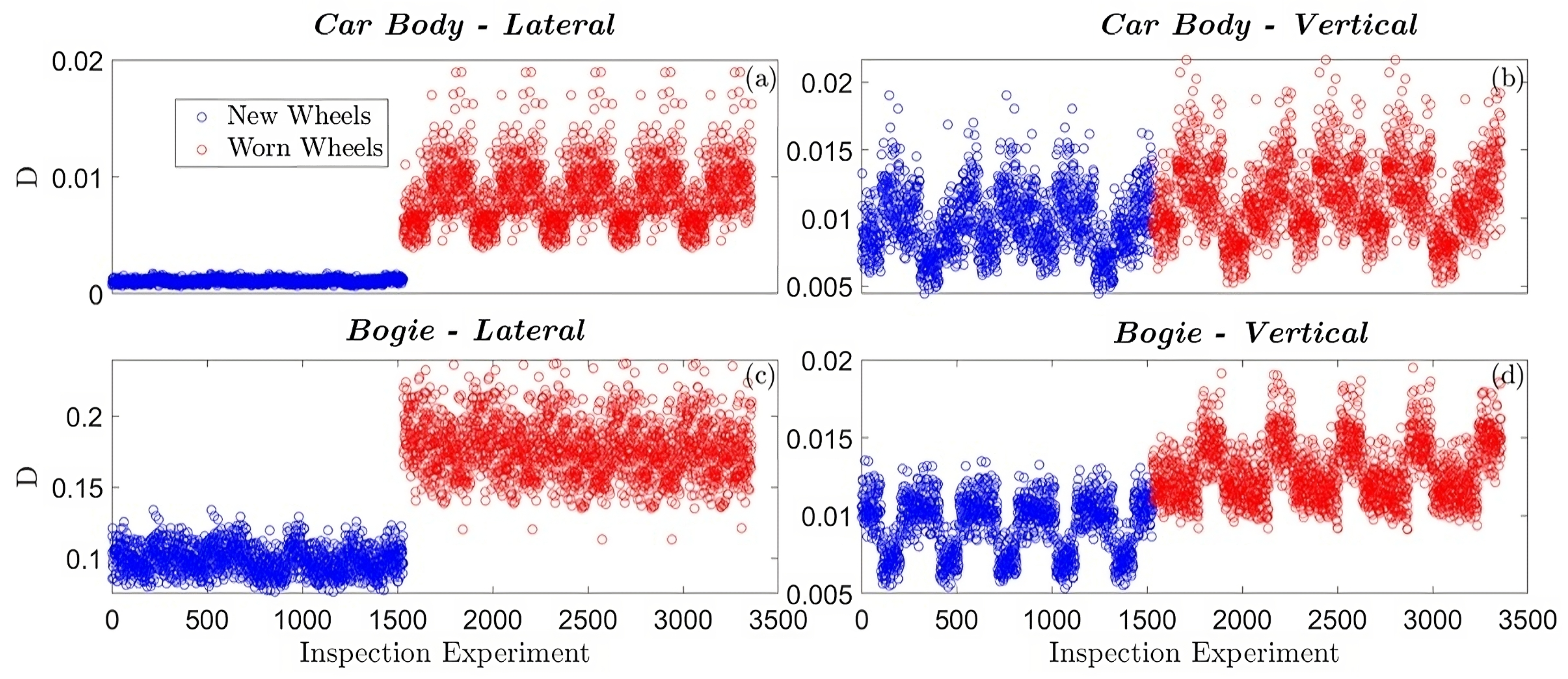
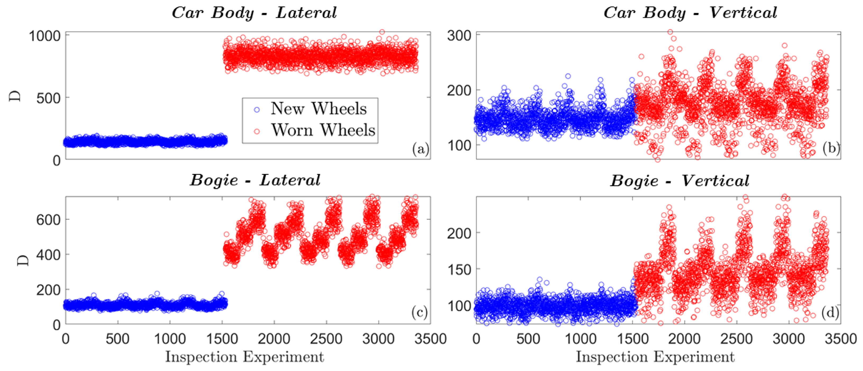
- Case Study A. Twenty signals (also see Table 3) per speed (60/70/80 km/h) are used in the baseline phase for the estimation of a corresponding number of AR models per sensor. The order (equal to parameter vector dimensionality) of each of the obtained AR models per sensor and related details are shown in Table 5, while the scatter-type plots of the method’s distance metric D and the corresponding ROC curves are illustrated in Figure 15 and Figure 18, respectively. Based on these, the method’s performance is characterized as follows:
Figure 18.
Case Study A—distance metric plot for the U-MM-AR method based on sensors (a) , (b) , (c) , (d) (3360 inspection test cases).
Figure 18.
Case Study A—distance metric plot for the U-MM-AR method based on sensors (a) , (b) , (c) , (d) (3360 inspection test cases).

The above results indicate that the U-MM-AR method achieves slightly better performance compared to the U-MM-PSD based on lateral measurements, while it is capable of detecting hollow worn wheels with vertical measurement to the bogie with quite high TPR.
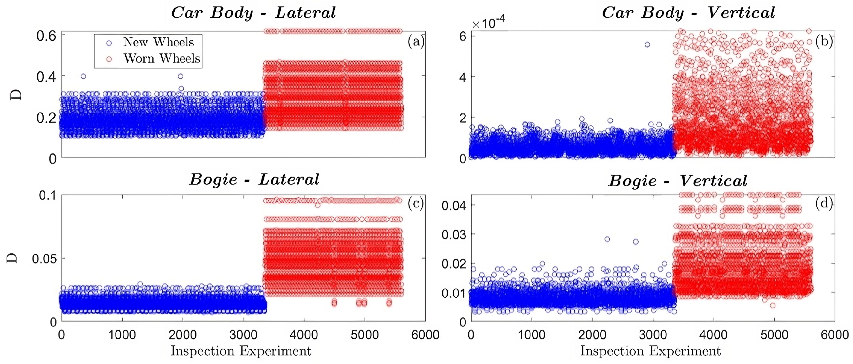
The performance of the U-MM-AR method is again assessed by scatter plots and ROC curves, which are displayed in Figure 19 and Figure 17, respectively. Based on these, the methods’ performance is characterized as follows:
Figure 19.
Case Study B—distance metric plot for the U-MM-AR method based on sensors (a) , (b) , (c) , (d) (5600 inspection test cases).
Figure 19.
Case Study B—distance metric plot for the U-MM-AR method based on sensors (a) , (b) , (c) , (d) (5600 inspection test cases).
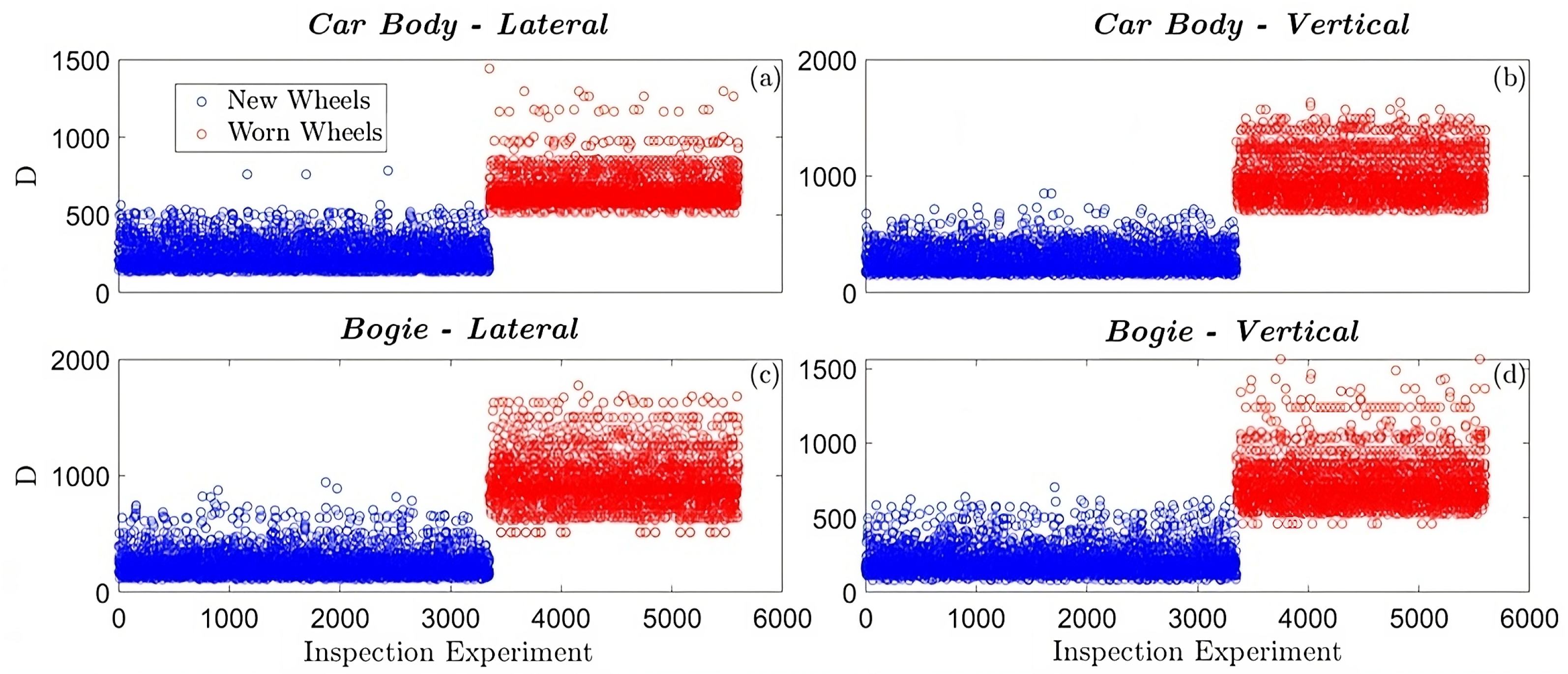
It is remarkable, that for all sensor measurements, the U-MM-AR method achieves TPR for false alarm rates under 5%.
7. Critical Discussion on the Results
Based on the results of Section 6, the best detection performance in Case Study A is achieved by both methods when the lateral carbody measurements () are used; TPR for FPR. However, only the U-MM-AR method achieves the same performance using the bogie lateral measurements (). In Case Study B, the U-MM-AR method detects hollow worn wheels with almost perfect performance in all test cases, with the best results achieved when carbody vertical measurements () are used: TPR for FPR. In the same case study, the U-MM-PSD achieves its best performance using lateral bogie measurements: TPR for FPR.
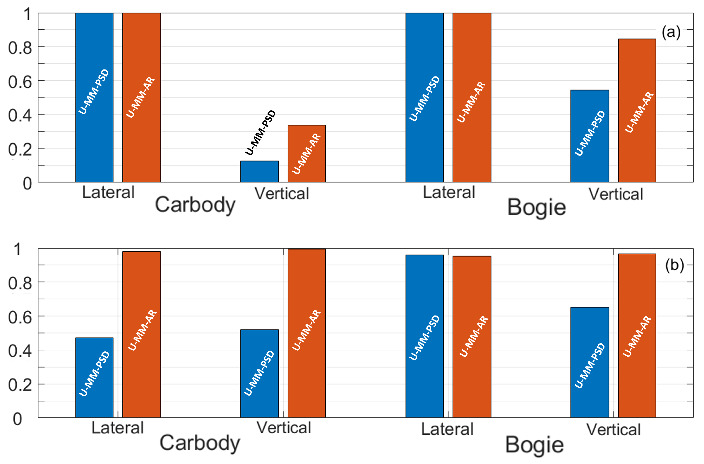
Summary detection results for both methods are illustrated in Figure 20 through a variant of the area under the ROC curve (AUC) [35]. The typical AUC may range from 0 to 1 with values approaching 1 indicating excellent detection performance (TPR ), while includes AUC values for higher FPR than . The “local AUC” that is used in this study indicates the method’s TPR for FPR values within the range of 0–5%, which is reasonable for practical applications, where high FPR values render a detection method unreliable. The “local AUC” is normalized within the 0–1 range in order to be interpreted as the typical AUC with the best performance indicated by values close to 1.
U-MM-PSD. The method achieves very good performance with lateral bogie measurements, while its performance is generally poor when vertical vibration signals are used due to the fact that hollow worn wheels affect mostly the lateral vehicle dynamics. It is worth noting that one of the important characteristics of this method is its simplicity and the need for low user expertise for its operation. However, the selection of the user-defined parameter k—number of frequencies with the minimum variance in the feature vector—needs user familiarization with the investigated system dynamics, while a starting point may be a k value, including the of the frequencies with the lower PSD sample variance that leads to optimal or near optimal detection performance.
U-MM-AR. This method has overall better detection performance than the U-MM-PSD, achieving excellent detection results in all considered field test cases (Case Study B), even using vertical vibration signals (Figure 20) from either the bogie or the carbody. This is due to the detailed parametric modeling of the vehicle healthy dynamics via the multiple AR models, which leads to the detection of additional, subtle, effects on the dynamics caused by the potential wheel OOR that frequently occurs together with wheel hollow wear (this applies only to Case Study B, where the wheels may potentially include additional defects) and primarily affects the vertical vehicle dynamics, as well as other minor effects of the wheel hollow wear of the vertical measurements. Nevertheless, caution and user expertise are necessary for the AR modeling for the best detection performance of the U-MM-AR method.
8. Conclusions
The on-board robust detection of hollow worn railway vehicle wheels under normal operating conditions and varying traveling speeds is accomplished in the present study within a multiple model framework via two unsupervised statistical time series (STS) methods. The detection is achieved at an early stage before the standard wheel hollow wear limit is reached, and the acquired vibration signals’ RMS values indicate hollow worn wheels. Both methods operate using vibration signals from a single accelerometer on the vertical or lateral direction of the bogie or the carbody, and their assessment and comparison are performed through a statistical reliable procedure, including two case studies and thousands of test cases. The first case study is based on Monte Carlo simulations and vibration signals obtained from a detailed 42-DOF railway vehicle model developed in SIMPACK, while the second is based on field experiments with an Athens Metro train. The U-MM-AR method presents the best overall performance, achieving the maximum correct detection rate (TPR) of for a false alarm rate (FPR) of with the following U-MM-PSD reaching a TPR of for FPR equal to .
In addition, the main lessons learned from the study are as follows:
- The detection of early-stage hollow worn wheels is a highly challenging problem, as the measured dynamics via vibration signals is significantly affected by the traveling speed and effects due to hollow wear potentially being fully “masked” by the effects due to speed variation.
- The lateral direction measurements of acceleration on the vehicle carbody and especially on the bogie are, as expected, more sensitive to wheel hollow wear, yet signals on the vertical direction may be used complementarily for the detection of other types of wheel defects.
- Advanced data-driven methods may effectively tackle the problem of railway vehicle worn wheels under different speeds using on-board random vibration measurements from even a single sensor. The prerequisite of such methods is their training via an adequate number of vibration signal batches from the vehicle traveling at normal operation speeds with healthy wheels.
Future plans include the assessment of the methods with other types of wheel defects, such as conicity and polygonization, as well as additional varying OCs, such as payload and track irregularity.
Author Contributions
Conceptualization, J.S.S. and S.D.F.; Methodology, N.K., J.S.S. and S.D.F.; Software, N.K.; Validation, N.K.; Formal analysis, N.K., J.S.S. and S.D.F.; Investigation, N.K., J.S.S. and S.D.F.; Resources, J.S.S. and S.D.F.; Data curation, N.K.; Writing—original draft, N.K. and J.S.S.; Writing—review & editing, J.S.S. and S.D.F.; Visualization, N.K.; Supervision, J.S.S. and S.D.F.; Project administration, S.D.F. and J.S.S.; Funding acquisition, S.D.F. and J.S.S. All authors have read and agreed to the published version of the manuscript.
Funding
This research has been partly funded by the European Union and Greek national funds through the Operational Program Competitiveness, Entrepreneurship and Innovation, under the call RESEARCH—CREATE—INNOVATE (project MAIANDROS; project code: T1EDK—01440).
Data Availability Statement
Not applicable.
Acknowledgments
Special thanks are due to I. Iliopoulos and G. Vlachospyros from the University of Patras for their help with the on-vehicle measurements, A. Deloukas, G. Leoutsakos, C. Giannakis, and I. Tountas of Attiko Metro S.A. for information on the vehicle and the wheels, as well as to C. Mamaloukakis, K. Katsiana, K. Sarris, G. Karagiannidis, S. Grammatikakis, P. Samaras, N. Barlabas, K. Doularidis, V. Maroufidis, A. Panagiotakis, K. Vranas, G. Bourotis, and A. Karatzas of STASY S.A. who provided technical support during the on-vehicle measurements. Thanks are due to T. Aravanis and K. Vamvoudakis of the University of Patras for fruitful discussions and G. Vlachospyros for his help on the final revision of the manuscript.
Conflicts of Interest
The authors declare no conflict of interest.
Appendix A. Details of the SIMPACK Railway Vehicle Model (Case Study A)
Figure A1.
The railway vehicle model (Case Study A): (a) side view, (b) top view.
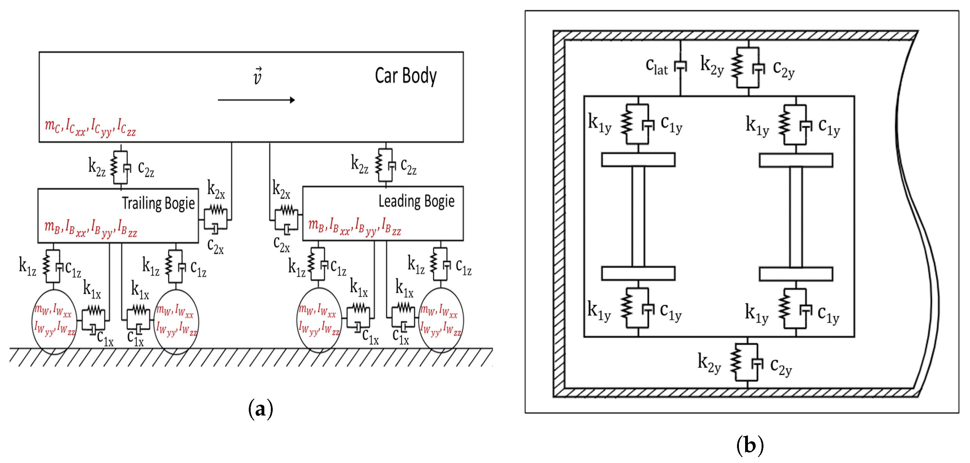
Table A1.
Railway vehicle model parameters (Case Study A).
| Parameter | Description | Value | Unit |
|---|---|---|---|
| Carbody mass | 19,529 | [kg] | |
| Bogie frame mass | 2049 | [kg] | |
| Wheelset mass | 2132 | [kg] | |
| Axle box mass | 30 | [kg] | |
| Carbody roll moment of inertia | 55,953 | [kg m2] | |
| Carbody pitch moment of inertia | 1,311,322 | [kg m2] | |
| Carbody yaw moment of inertia | 1,309,593 | [kg m2] | |
| Bogie roll moment of inertia | 1314 | [kg m2] | |
| Bogie pitch moment of inertia | 1470 | [kg m2] | |
| Bogie yaw moment of inertia | 2660 | [kg m2] | |
| Wheelset roll moment of inertia | 474 | [kg m2] | |
| Wheelset pitch moment of inertia | 30 | [kg m2] | |
| Wheelset yaw moment of inertia | 474 | [kg m2] | |
| Carbody width | 2 | [m] | |
| Carbody length | 17 | [m] | |
| Distance between center of gravity (c.g.) of carbody | |||
| and c.g. of bogie | [m] | ||
| Distance between wheelsets in a bogie (wheelbase) | [m] | ||
| Wheel rolling circle diameter | 860 | [mm] | |
| Rail inclination | 1:20 | ||
| Wheel profile | S1002 | ||
| Rail profile | UIC54 | ||
| Prim.Sups. Longitudinal Stiffness | kN/mm | ||
| Prim.Sups. Lateral Stiffness | kN/mm | ||
| Prim.Sups. Longitudinal Stiffness | kN/mm | ||
| Prim.Sups. Longitudinal Damping | 20 | kN·s/m | |
| Prim.Sups. Lateral Damping | 15 | kN·s/m | |
| Prim.Sups. Vertical Damping | 12 | kN·s/m | |
| Sec.Sups. Longitudinal Stiffness | kN/mm | ||
| Sec.Sups. Lateral Stiffness | kN/mm | ||
| Sec.Sups. Longitudinal Stiffness | kN/mm | ||
| Sec.Sups. Longitudinal Damping | 10 | kN·s/m | |
| Sec.Sups. Lateral Damping | 10 | kN·s/m | |
| Sec.Sups. Vertical Damping | 10 | kN·s/m | |
| Lateral Damper Damping | 50 | kN·s/m | |
| v | Vehicle Speed | km/h |
Appendix B. Important Symbols and Acronyms
| Important Symbols | Acronyms | ||
| j-th AR (scalar) parameter | AR | Autoregressive (model) | |
| distance between the models and | BIC | Bayesian Information Criterion | |
| D | distance metric used in the MM methods | AUC | Area Under the ROC Curve |
| AR model order | |||
| railway vehicle wheel diameter | OCs | Operating Conditions | |
| i-th AR model residual signal | TPR | True Positive Rate | |
| sampling frequency | FPR | False Positive Rate | |
| cut-off frequency | MM | Multiple Model | |
| wheel rotation frequency | NID | Normally Independently | |
| Distributed | |||
| k | number of frequencies retained in | OOR | Out-Of-Roundness |
| the U-MM-PSD method | |||
| carbody lateral/vertical vibration measurements | PHM | Prognostics and Health | |
| bogie lateral/vertical vibration measurements | Management | ||
| n | MM dimensionality | PSD | Power Spectral Density |
| i-th model representing the vehicle dynamics | RMS | Root Mean Square | |
| corresponding to healthy wheels | |||
| model representing the vehicle dynamics | RSS | Residual Sum of Squares | |
| under unknown speed and wheels condition | |||
| N | vibration signal length (samples) | SSS | Series Sum of Squares |
| normalized by the sampling period | SPP | Samples Per Parameter | |
| discrete time | |||
| vibration response signal from the vehicle | STS | Statistical Time Series | |
| under unknown speed and wheels condition | |||
| i-th AR model parameter vector corresponding | |||
| to model | U-MM-AR | Unsupervised Multiple Model | |
| covariance matrix of | Autoregressive parameter | ||
| based method | |||
| AR model parameter vector corresponding | U-MM-PSD | Unsupervised Multiple Model | |
| to model | Power Spectral Density | ||
| covariance matrix of | based method | ||
References
- Jardine, A.K.; Lin, D.; Banjevic, D. A review on machinery diagnostics and prognostics implementing condition-based maintenance. Mech. Syst. Signal Process. 2006, 20, 1483–1510. [Google Scholar] [CrossRef]
- Polach, O.; Nicklisch, D. Wheel/rail contact geometry parameters in regard to vehicle behaviour and their alteration with wear. Wear 2016, 366–367, 200–208. [Google Scholar] [CrossRef]
- Soleimani, H. Tribological Aspects of Wheel—Rail Contact: A Review of Wear Mechanisms and Effective Factors on Rolling Contact Fatigue. Urban Rail Transit 2017, 3, 227–237. [Google Scholar] [CrossRef]
- Asplund, M.; Palo, M.; Famurewa, S.; Rantatalo, M. A study of railway wheel profile parameters used as indicators of an increased risk of wheel defects. Proc. Inst. Mech. Eng. Part F J. Rail Rapid Transit 2016, 230, 323–334. [Google Scholar] [CrossRef]
- Jin, X.; Wu, L.; Fang, J.; Zhong, S.; Ling, L. An investigation into the mechanism of the polygonal wear of metro train wheels and its effect on the dynamic behaviour of a wheel/rail system. Veh. Syst. Dyn. 2012, 50, 1817–1834. [Google Scholar] [CrossRef]
- Jia, S.; Dhanasekar, M. Detection of Rail Wheel Flats using Wavelet Approaches. Struct. Health Monit. 2007, 6, 121–131. [Google Scholar] [CrossRef]
- Liang, B.; Iwnicki, S.; Ball, A.; Young, A. Adaptive noise cancelling and time—Frequency techniques for rail surface defect detection. Mech. Syst. Signal Process. 2015, 54–55, 41–51. [Google Scholar] [CrossRef]
- Zhang, J.; Gao, H.; Liu, Q.; Farzadpour, F.; Grebe, C.; Tian, Y. Adaptive parameter blind source separation technique for wheel condition monitoring. Mech. Syst. Signal Process. 2017, 90, 208–221. [Google Scholar] [CrossRef]
- Ye, Y.; Shi, D.; Krause, P.; Hecht, M. A data-driven method for estimating wheel flat length. Veh. Syst. Dyn. 2020, 58, 1329–1347. [Google Scholar] [CrossRef]
- Nielsen, J.C.O.; Johansson, A. Out-of-round railway wheels-a literature survey. Proc. Inst. Mech. Eng. Part F J. Rail Rapid Transit 2000, 214, 79–91. [Google Scholar] [CrossRef]
- Sun, Q.; Chen, C.; Kemp, A.H.; Brooks, P. An on-board detection framework for polygon wear of railway wheel based on vibration acceleration of axle-box. Mech. Syst. Signal Process. 2021, 153, 107540. [Google Scholar] [CrossRef]
- Zeng, D.; Xu, T.; Wang, J.; Lu, L.; Meng, W.; Jiang, B.; Zou, Q. Investigation of the crack initiation of subsurface rolling contact fatigue in railway wheels. Int. J. Fatigue 2020, 130, 105281. [Google Scholar] [CrossRef]
- Kato, T.; Fujimura, T.; Yamamoto, Y.; Dedmon, S.; Hiramatsu, S.; Kato, H.; Kimura, Y.; Pilch, J. Critical internal defect size for subsurface crack initiation in heavy haul car wheels. Wear 2019, 438–439, 203038. [Google Scholar] [CrossRef]
- Pau, M.; Leban, B.; Baldi, A. Simultaneous subsurface defect detection and contact parameter assessment in a wheel—Rail system. Wear 2008, 265, 1837–1847. [Google Scholar] [CrossRef]
- Sutharssan, T.; Stoyanov, S.; Bailey, C.; Yin, C. Prognostic and health management for engineering systems: A review of the data-driven approach and algorithms. J. Eng. 2015, 2015, 215–222. [Google Scholar] [CrossRef]
- Gasparetto, L.; Alfi, S.; Bruni, S. Data-driven condition-based monitoring of high-speed railway bogies. Int. J. Rail Transp. 2013, 1, 42–56. [Google Scholar] [CrossRef]
- Papaelias, M.; Amini, A.; Huang, Z.; Vallely, P.; Dias, D.C.; Kerkyras, S. Online condition monitoring of rolling stock wheels and axle bearings. Proc. Inst. Mech. Eng. Part F J. Rail Rapid Transit 2016, 230, 709–723. [Google Scholar] [CrossRef]
- Wang, Y.; Ni, Y.; Wang, X. Real-time defect detection of high-speed train wheels by using Bayesian forecasting and dynamic model. Mech. Syst. Signal Process. 2020, 139, 106654. [Google Scholar] [CrossRef]
- Ward, C.P.; Weston, P.F.; Stewart, E.J.C.; Li, H.; Goodall, R.M.; Roberts, C.; Mei, T.X.; Charles, G.; Dixon, R. Condition Monitoring Opportunities Using Vehicle-Based Sensors. Proc. Inst. Mech. Eng. Part F J. Rail Rapid Transit 2011, 225, 202–218. [Google Scholar] [CrossRef]
- Fröhling, R.; Ekberg, A.; Kabo, E. The detrimental effects of hollow wear—Field experiences and numerical simulations. Wear 2008, 265, 1283–1291. [Google Scholar] [CrossRef]
- Sawley, K.; Wu, H. The formation of hollow-worn wheels and their effect on wheel/rail interaction. Wear 2005, 258, 1179–1186. [Google Scholar] [CrossRef]
- Sawley, K.; Urban, C.; Walker, R. The effect of hollow-worn wheels on vehicle stability in straight track. Wear 2005, 258, 1100–1108. [Google Scholar] [CrossRef]
- Pires, A.; Pacheco, L.; Dalvi, I.; Endlich, C.; Queiroz, J.; Antoniolli, F.; Santos, G. The effect of railway wheel wear on reprofiling and service life. Wear 2021, 477, 203799. [Google Scholar] [CrossRef]
- Zhai, W.; Liu, P.; Lin, J.; Wang, K. Experimental investigation on vibration behaviour of a CRH train at speed of 350 km/h. Int. J. Rail Transp. 2015, 3, 1–16. [Google Scholar] [CrossRef]
- Wang, J.; Song, C.; Wu, P.; Dai, H. Wheel reprofiling interval optimization based on dynamic behavior evolution for high speed trains. Wear 2016, 366–367, 316–324. [Google Scholar] [CrossRef]
- Shi, H.; Wang, J.; Wu, P.; Song, C.; Teng, W. Field measurements of the evolution of wheel wear and vehicle dynamics for high-speed trains. Veh. Syst. Dyn. 2018, 56, 1187–1206. [Google Scholar] [CrossRef]
- Wu, X.; Rakheja, S.; Wu, H.; Qu, S.; Wu, P.; Dai, H.; Zeng, J.; Ahmed, A.K.W. A study of polygonal wheel wear through a field test programme. Veh. Syst. Dyn. 2019, 57, 914–934. [Google Scholar] [CrossRef]
- Charles, G.; Goodall, R.; Dixon, R. Model-based condition monitoring at the wheel—Rail interface. Veh. Syst. Dyn. 2008, 46, 415–430. [Google Scholar] [CrossRef]
- Aravanis, T.C.; Sakellariou, J.; Fassois, S. A stochastic Functional Model based method for random vibration based robust fault detection under variable non—Measurable operating conditions with application to railway vehicle suspensions. J. Sound Vib. 2020, 466, 115006. [Google Scholar] [CrossRef]
- Vamvoudakis-Stefanou, K.; Sakellariou, J.; Fassois, S. Vibration-based damage detection for a population of nominally identical structures: Unsupervised Multiple Model (MM) statistical time series type methods. Mech. Syst. Signal Process. 2018, 111, 149–171. [Google Scholar] [CrossRef]
- Ljung, L. System Identification: Theory for the User, 2nd ed.; Prentice–Hall: Hoboken, NJ, USA, 1999. [Google Scholar]
- Press, W.; Teukolsky, S.; Vetterling, W.; Flannery, B. Numerical Recipes: The Art of Scientific Computing, 3rd ed.; Cambridge University Press: Cambridge, UK, 2007. [Google Scholar]
- Rulka, W. SIMPACK—A Computer Program for Simulation of Large-motion Multibody Systems. In Multibody Systems Handbook; Schiehlen, W., Ed.; Springer: Berlin/Heidelberg, Germany, 1990; pp. 265–284. [Google Scholar] [CrossRef]
- Duda, R.; Hart, P.; Stork, D. Pattern Classification, 2nd ed.; John Wiley & Sons: New York, NY, USA, 2000. [Google Scholar]
- Fawcett, T. An introduction to ROC analysis. Pattern Recognit. Lett. 2006, 27, 861–874. [Google Scholar] [CrossRef]
- Kaliorakis, N.; Iliopoulos, I.A.; Vlachospyros, G.; Sakellariou, J.S.; Fassois, S.D.; Deloukas, A.; Leoutsakos, G.; Chronopoulos, E.; Mamaloukakis, C.; Katsiana, K. On the On–Board Random Vibration–Based Detection of Hollow Worn Wheels in Operating Railway Vehicles. In European Workshop on Structural Health Monitoring (EWSHM); Rizzo, P., Milazzo, A., Eds.; Springer: Cham, Switzerland, 2021; pp. 480–489. [Google Scholar] [CrossRef]
- Simpack 2023. Available online: https://www.3ds.com/products-services/simulia/products/simpack/product-modules/rail-modules (accessed on 24 September 2023).
- Polach, O.; Bottcher, A.; Vannucci, D.; Sima, J.; Schelle, H.; Chollet, H.; Gotz, G.; Prada, M.G.; Nicklisch, D.; Mazzola, L.; et al. Validation of simulation models in the context of railway vehicle acceptance. Proc. Inst. Mech. Eng. Part F J. Rail Rapid Transit 2015, 229, 729–754. [Google Scholar] [CrossRef]
- Ye, Y.; Zhang, Y.; Wang, Q.; Wang, Z.; Teng, Z.; Zhang, H. Fault diagnosis of high-speed train suspension systems using multiscale permutation entropy and linear local tangent space alignment. Mech. Syst. Signal Process. 2020, 138, 106565. [Google Scholar] [CrossRef]
- Hou, M.; Chen, B.; Cheng, D. Study on the Evolution of Wheel Wear and Its Impact on Vehicle Dynamics of High-Speed Trains. Coatings 2022, 12, 1333. [Google Scholar] [CrossRef]
- Schupp, G. Bifurcation Analysis of Railway Vehicles. Multibody Syst. Dyn. 2006, 15, 25–50. [Google Scholar] [CrossRef]
- Gadhave, R.; Vyas, N.S. Rail-wheel contact forces and track irregularity estimation from on-board accelerometer data. Veh. Syst. Dyn. 2022, 60, 2145–2166. [Google Scholar] [CrossRef]
- Haigermoser, A.; Luber, B.; Rauh, J.; Gräfe, G. Road and track irregularities: Measurement, assessment and simulation. Veh. Syst. Dyn. 2015, 53, 878–957. [Google Scholar] [CrossRef]
- Kalker, J.J. A Fast Algorithm for the Simplified Theory of Rolling Contact. Veh. Syst. Dyn. 1982, 11, 1–13. [Google Scholar] [CrossRef]
- Iliopoulos, I.A.; Sakellariou, J.S.; Fassois, S.D. Parametric spectral estimation and dynamics identification for a traveling surface vehicle. In Proceedings of the 11th International Conference on Structural Dynamics (EURODYN2020), Athens, Greece, 23–26 November 2020; pp. 1–12. [Google Scholar] [CrossRef]
- Tao, G.; Wen, Z.; Liang, X.; Ren, D.; Jin, X. An investigation into the mechanism of the out-of-round wheels of metro train and its mitigation measures. Veh. Syst. Dyn. 2019, 57, 1–16. [Google Scholar] [CrossRef]
- Bishop, C.M. Pattern Recognition and Machine Learning; Springer Science + Business Media, LLC.: New York, NY, USA, 2006. [Google Scholar]
Figure 1.
Details of the SIMPACK railway vehicle model and the sensor positions. (a) Side view of the vehicle, (b) zoomed-in view of the front bogie and the suspensions, (c) bottom view of the vehicle.
Figure 1.
Details of the SIMPACK railway vehicle model and the sensor positions. (a) Side view of the vehicle, (b) zoomed-in view of the front bogie and the suspensions, (c) bottom view of the vehicle.

Figure 2.
Case Study A—new (healthy) and hollow worn wheel profiles.
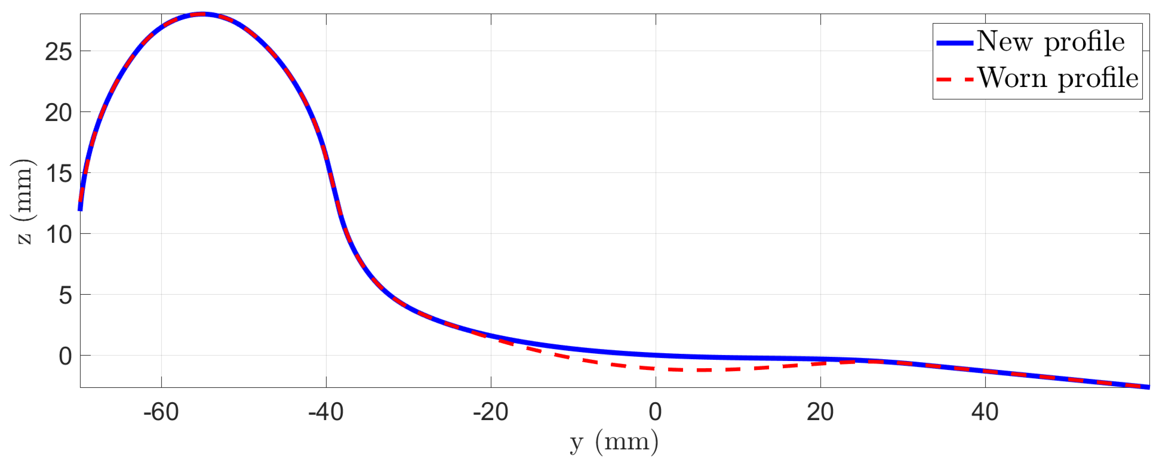
Figure 3.
Case Study A—indicative vibration signals for vehicle speed of 80 km/h based on sensors: (a) , (b) , (c) , (d) .
Figure 3.
Case Study A—indicative vibration signals for vehicle speed of 80 km/h based on sensors: (a) , (b) , (c) , (d) .
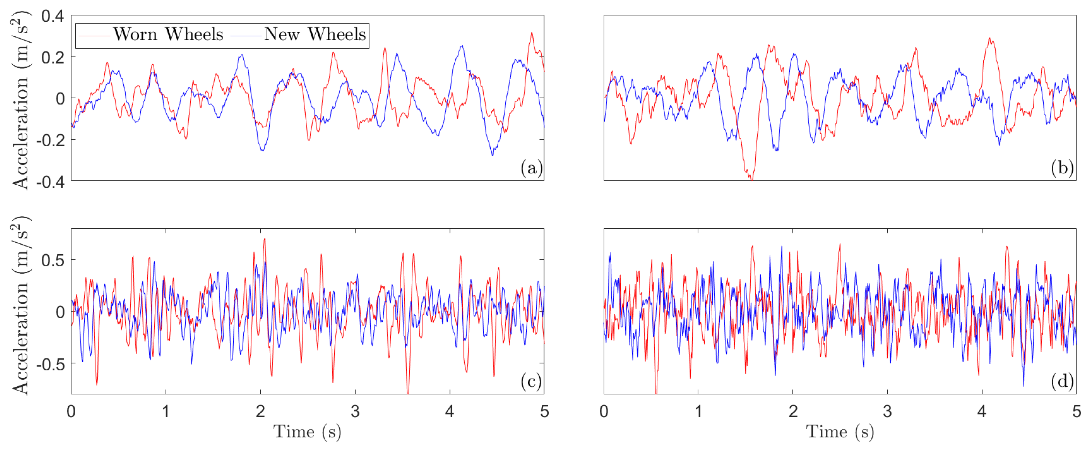
Figure 4.
Case Study A—box plots of vibration signals RMS values for all considered speeds and wheel conditions based on sensors: (a) , (b) , (c) , (d) . The top and bottom of each box are the 25th and 75th percentiles, while the distance between the top and bottom is the interquartile range. The red line in the middle of each box is the sample median, and the lines extending above and below each box are the whiskers. These are drawn from the ends of the interquartile range, and their length is 1.5 times the interquartile range. The red crosses represent observations beyond the whiskers (outliers).

Figure 5.
Case Study A—effects of speed variability on Welch-based PSD estimates corresponding to new wheels using vibration signals from sensors: (a) , (b) (122 signals per vehicle speed). The indicated frequencies correspond to the periodic wheelbase-filtering effect per speed.
Figure 5.
Case Study A—effects of speed variability on Welch-based PSD estimates corresponding to new wheels using vibration signals from sensors: (a) , (b) (122 signals per vehicle speed). The indicated frequencies correspond to the periodic wheelbase-filtering effect per speed.

Figure 6.
Case Study A—Welch-based PSD estimates corresponding to vehicle with new and hollow worn wheels that travels at a speed of 60 km/h using vibration signals from sensors: (a) , (b) , (c) , (d) (122 signals per wheel condition).
Figure 6.
Case Study A—Welch-based PSD estimates corresponding to vehicle with new and hollow worn wheels that travels at a speed of 60 km/h using vibration signals from sensors: (a) , (b) , (c) , (d) (122 signals per wheel condition).
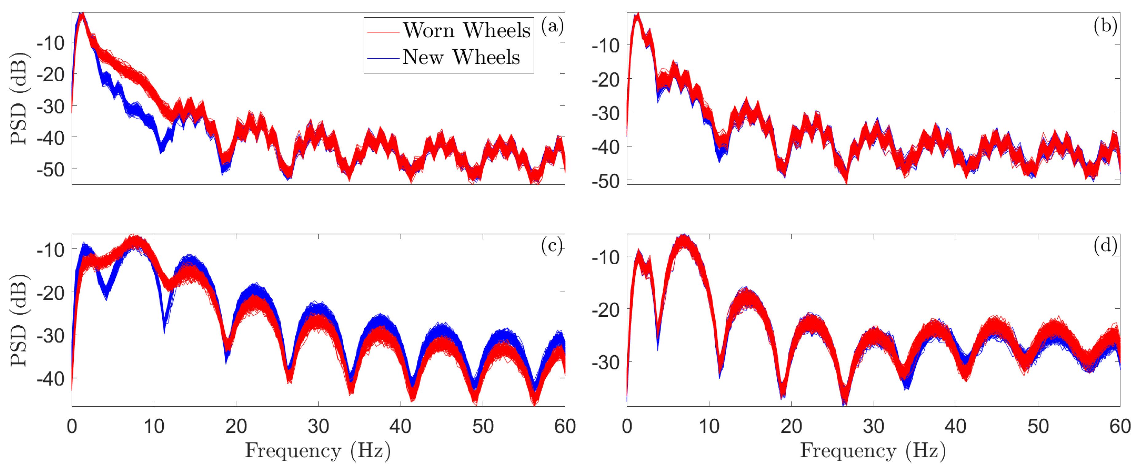
Figure 7.
Case Study A—effects of speed variability (60, 70, and 80 km/h) and wheel condition on Welch-based PSD envelopes using all measured vibration signals from sensors: (a) , (b) , (c) , (d) .
Figure 7.
Case Study A—effects of speed variability (60, 70, and 80 km/h) and wheel condition on Welch-based PSD envelopes using all measured vibration signals from sensors: (a) , (b) , (c) , (d) .

Figure 8.
Case Study B—photo of the Athens Metro vehicle and the installed sensors. Two uniaxial accelerometers used for and (left) and one tri-axial accelerometer for and (right).
Figure 8.
Case Study B—photo of the Athens Metro vehicle and the installed sensors. Two uniaxial accelerometers used for and (left) and one tri-axial accelerometer for and (right).
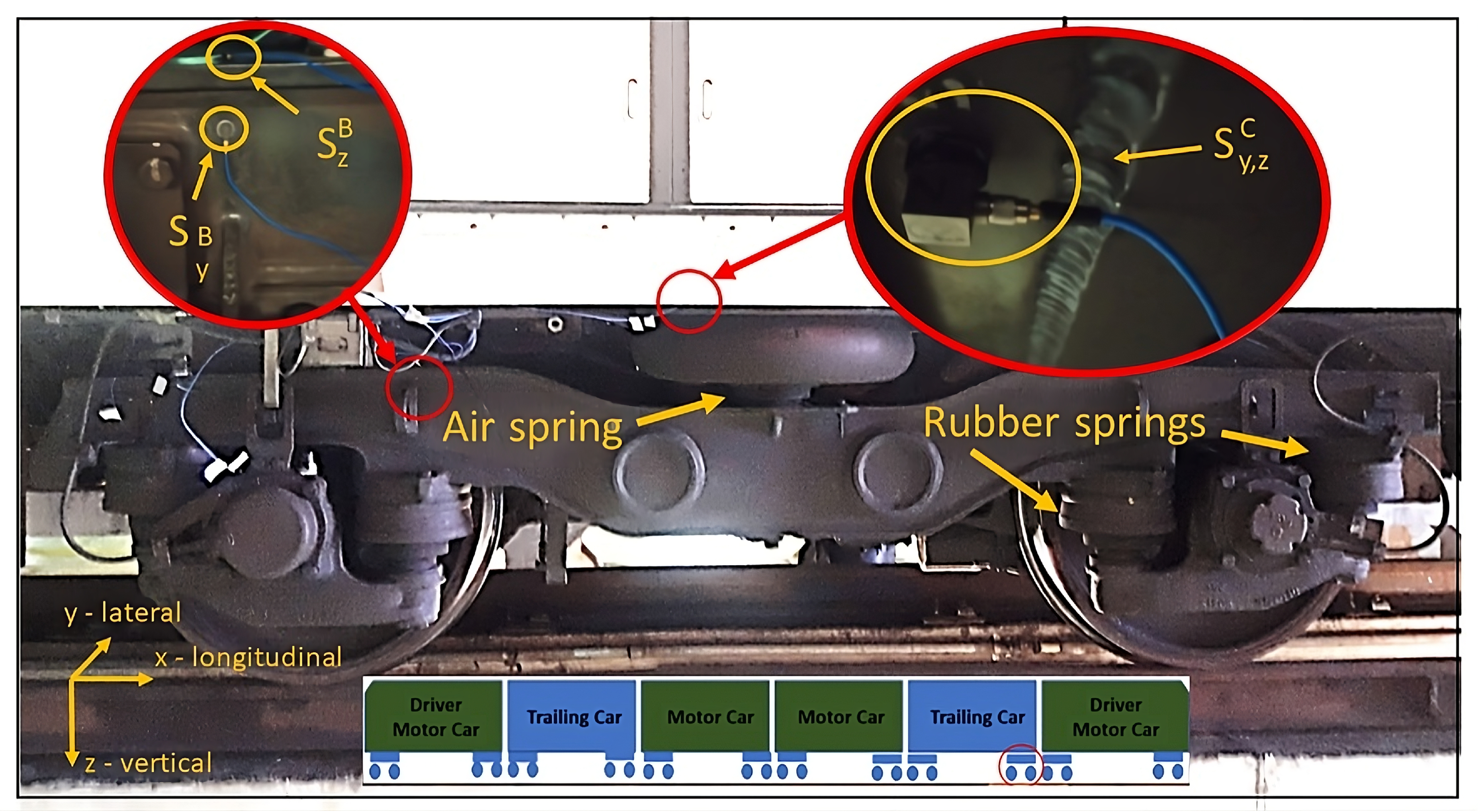
Figure 9.
Case Study B—indicative vibration signals for vehicle speed 80 km/h based on sensors: (a) , (b) , (c) , (d) .
Figure 9.
Case Study B—indicative vibration signals for vehicle speed 80 km/h based on sensors: (a) , (b) , (c) , (d) .

Figure 10.
Case Study B—box plots of vibration signals RMS values for all considered speeds and wheel conditions based on sensors: (a) , (b) , (c) , and (d) . The top and bottom of each box are the 25th and 75th percentiles, while the distance between the top and bottom is the interquartile range. The red line in the middle of each box is the sample median, and the lines extending above and below each box are the whiskers. These are drawn from the ends of the interquartile range, and their length is 1.5 times the interquartile range. The red crosses represent observations beyond the whiskers (outliers).

Figure 11.
Case Study B—effects of speed variability on Welch-based PSD envelopes corresponding to new wheels using vibration signals from sensors: (a) , (b) (all available signals per vehicle speed). The indicated frequencies correspond to the respective wheel harmonics.
Figure 11.
Case Study B—effects of speed variability on Welch-based PSD envelopes corresponding to new wheels using vibration signals from sensors: (a) , (b) (all available signals per vehicle speed). The indicated frequencies correspond to the respective wheel harmonics.

Figure 12.
Case Study B—Welch-based PSD envelopes corresponding to vehicle with new and hollow worn wheels that travels with speed of 70 km/h from sensors: (a) , (b) , (c) , (d) (all available signals per speed and wheel condition). The indicated frequencies correspond to the respective wheel harmonics, attributed to potential wheel out-of-roundness.
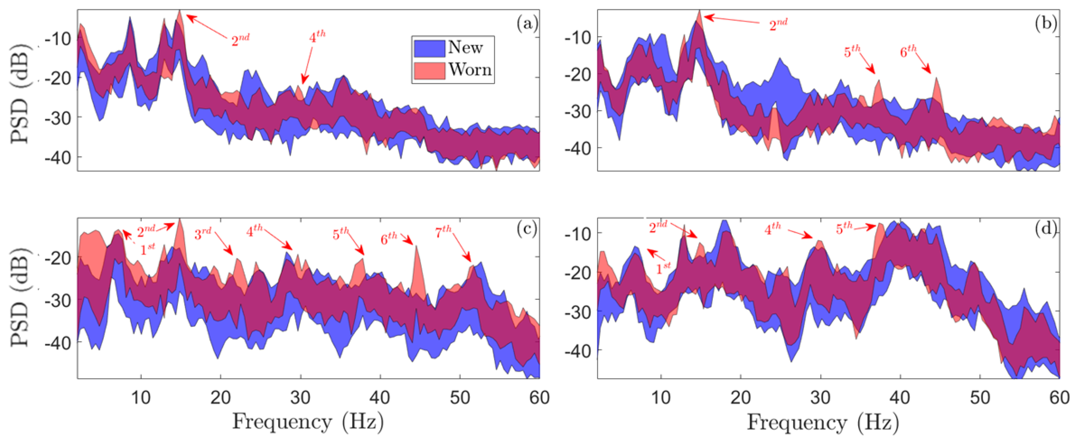
Figure 13.
Case Study B—effects of speed variability (60, 70, and 80 km/h) and wheel condition on Welch-based PSD envelopes using all measured vibration signals from sensors: (a) , (b) , (c) , (d) .
Figure 13.
Case Study B—effects of speed variability (60, 70, and 80 km/h) and wheel condition on Welch-based PSD envelopes using all measured vibration signals from sensors: (a) , (b) , (c) , (d) .

Figure 20.
Summary of hollow worn wheel detection results based on the U-MM-PSD and U-MM-AR methods via the “local AUC”: (a) Case Study A, (b) Case Study B.
Figure 20.
Summary of hollow worn wheel detection results based on the U-MM-PSD and U-MM-AR methods via the “local AUC”: (a) Case Study A, (b) Case Study B.

Table 1.
Case Study A—details of the vibration signals with respect to vehicle speed and wheel condition (for each sensor).
Table 1.
Case Study A—details of the vibration signals with respect to vehicle speed and wheel condition (for each sensor).
| Vehicle Speed (km/h) | No. of Signals | |
|---|---|---|
| New Wheels | Worn Wheels | |
| 60 | 122 | 122 |
| 70 | 122 | 122 |
| 80 | 122 | 122 |
| Total | 366 | 366 |
| Sampling frequency: Hz; operational bandwidth: 0–60 Hz; | ||
| signal length: N = 6001 samples (50 s) | ||
Table 2.
Case Study B—details on the vibration signals with respect to vehicle speed and wheel condition (for each sensor).
Table 2.
Case Study B—details on the vibration signals with respect to vehicle speed and wheel condition (for each sensor).
| Vehicle Speed (km/h) | No. of Signals | |
|---|---|---|
| New Wheels | Worn Wheels | |
| 60 | 59 | 17 |
| 70 | 38 | 16 |
| 80 | 30 | 12 |
| Total | 127 | 45 |
| Sampling frequency: Hz; operational bandwidth: 2–60 Hz, | ||
| signal length: N = 10,000 samples (∼10.20 s) | ||
Table 3.
Case Study A—details on the rotation assessment procedure. Number of new wheel signals per speed used in the baseline phase (b), new wheel signals used in the inspection phase (), worn wheel signals used in the inspection phase (f), and aggregated inspection test cases after the implemented rotations (). The same numbers are used for all sensors.
| Vehicle Speed (km/h) | Baseline (New Wheels) () | Inspection (New Wheels) () | Inspection (Worn Wheels) () | Aggregated Inspection Test Cases ( *) |
|---|---|---|---|---|
| 60 | 20 | 102 | 122 | 1120 |
| 70 | 20 | 102 | 122 | 1120 |
| 80 | 20 | 102 | 122 | 1120 |
| Total | 60 | 306 | 366 | 3360 |
* q number of rotations: 5, inspection cases: .
Table 4.
Case Study B—details on the rotation assessment procedure. Number of new wheel signals per speed used in the baseline phase (b), new wheel signals used in the inspection phase (), worn wheel signals used in the inspection phase (f), and aggregated inspection test cases after the implemented rotations (). The same numbers are used for all sensors.
| Vehicle Speed (km/h) | Baseline (New Wheels) () | Inspection (New Wheels) () | Inspection (Worn Wheels) () | Aggregated Inspection Test Cases () * |
|---|---|---|---|---|
| 60 | 20 | 39 | 17 | 2800 |
| 70 | 20 | 18 | 16 | 1700 |
| 80 | 20 | 10 | 12 | 1000 |
| Total | 60 | 67 | 45 | 5600 |
* q number of rotations: 50, inspection cases: .
Disclaimer/Publisher’s Note: The statements, opinions and data contained in all publications are solely those of the individual author(s) and contributor(s) and not of MDPI and/or the editor(s). MDPI and/or the editor(s) disclaim responsibility for any injury to people or property resulting from any ideas, methods, instructions or products referred to in the content. |
© 2023 by the authors. Licensee MDPI, Basel, Switzerland. This article is an open access article distributed under the terms and conditions of the Creative Commons Attribution (CC BY) license (https://creativecommons.org/licenses/by/4.0/).
Share and Cite
MDPI and ACS Style
Kaliorakis, N.; Sakellariou, J.S.; Fassois, S.D. On-Board Random Vibration-Based Robust Detection of Railway Hollow Worn Wheels under Varying Traveling Speeds. Machines 2023, 11, 933. https://doi.org/10.3390/machines11100933
AMA Style
Kaliorakis N, Sakellariou JS, Fassois SD. On-Board Random Vibration-Based Robust Detection of Railway Hollow Worn Wheels under Varying Traveling Speeds. Machines. 2023; 11(10):933. https://doi.org/10.3390/machines11100933
Chicago/Turabian StyleKaliorakis, Nikolaos, John S. Sakellariou, and Spilios D. Fassois. 2023. "On-Board Random Vibration-Based Robust Detection of Railway Hollow Worn Wheels under Varying Traveling Speeds" Machines 11, no. 10: 933. https://doi.org/10.3390/machines11100933
Note that from the first issue of 2016, this journal uses article numbers instead of page numbers. See further details here.