Improved Fault Classification and Localization in Power Transmission Networks Using VAE-Generated Synthetic Data and Machine Learning Algorithms

Abstract

The reliable operation of power transmission networks depends on the timely detection and localization of faults. Fault classification and localization in electricity transmission networks can be challenging because of the complicated and dynamic nature of the system. In recent years, a variety of machine learning (ML) and deep learning algorithms (DL) have found applications in the enhancement of fault identification and classification within power transmission networks. Yet, the efficacy of these ML architectures is profoundly dependent upon the abundance and quality of the training data. This intellectual explanation introduces an innovative strategy for the classification and pinpointing of faults within power transmission networks. This is achieved through the utilization of variational autoencoders (VAEs) to generate synthetic data, which in turn is harnessed in conjunction with ML algorithms. This approach encompasses the augmentation of the available dataset by infusing it with synthetically generated instances, contributing to a more robust and proficient fault recognition and categorization system. Specifically, we train the VAE on a set of real-world power transmission data and generate synthetic fault data that capture the statistical properties of real-world data. To overcome the difficulty of fault diagnosis methodology in three-phase high voltage transmission networks, a categorical boosting (Cat-Boost) algorithm is proposed in this work. The other standard machine learning algorithms recommended for this study, including Support Vector Machine (SVM), Decision Trees (DT), Random Forest (RF), and K-Nearest Neighbors (KNN), utilizing the customized version of forward feature selection (FFS), were trained using synthetic data generated by a VAE. The results indicate exceptional performance, surpassing current state-of-the-art techniques, in the tasks of fault classification and localization. Notably, our approach achieves a remarkable 99% accuracy in fault classification and an extremely low mean absolute error (MAE) of 0.2 in fault localization. These outcomes represent a notable advancement compared to the most effective existing baseline methods.

1. Introduction

Electrical power transmission networks are susceptible to faults and failures. Power transmission networks are now becoming extremely critical infrastructures that deliver electricity from power plants to households and businesses, and sudden abnormal conditions on these networks can cause power outages, damage to costly equipment, and even serious safety hazards. The rapidly growing demand for electric power is increasing the complexity of power networks day by day. The abnormal condition occurs due to different reasons like environmental, accidental, incidental, and aging factors also responsible for the occurrence of faults. Any type of abnormal condition on the transmission line can damage the system in both directions, i.e., generation and utilization. Power transmission network fault analysis is a major subject under investigation in the field of predictive maintenance [1,2]. In the field of power transmission networks, the detection and localization of faults is very important and advanced signal processing techniques for that purpose are gaining heightened popularity. Machine learning frameworks rely on the concept that systems should undergo training based on statistical data and mathematical models to identify fault patterns with minimal human intervention [3]. Hence, the implementation of cutting-edge machine learning algorithms with extensive datasets becomes imperative due to the progress in intellectual electronic integration within smart grids. This will pave the way for the deployment of precise and reliable ML structures for the detection of abnormal conditions [4]. Figure 1 shows the illustrative demonstration of two-terminal transmission networks for transmitting power from generating sources to multiple types of loads and the occurrence of abnormal conditions on it.

Various types of techniques, such as wavelet analysis, genetic algorithm (GA), phasor measurement unit (PMU), and multi-information-based techniques are extensively used in the literature for the categorization of abnormal conditions on power transfer lines. Traditionally, fault diagnosis and localization in power transmission networks have been performed using rule-based or model-based approaches that require a detailed understanding of the network topology and fault characteristics [5,6]. However, the advent of artificial intelligence approaches is replacing the trade-off methodologies, which are incredibly time-consuming, and their accuracy is limited due to the complexity of the networks and variability of fault conditions. Tracing abnormal conditions by implementing machine learning and deep learning architectures on power transmission networks is a research area that aims to develop accurate and efficient algorithms for predictive maintenance compared to conventional techniques [7,8]. Figure 2 shows the overview to diagnose faults on transmission lines.

Unfortunately, acquiring labeled data poses significant challenges and time constraints, particularly within power systems where abnormal conditions are infrequent and often unpredictable. To address this issue, recent studies have investigated the potential of utilizing synthetically generated data to enhance the performance of ML architecture. Specifically, (GANs) and variational encoders (VAEs) have been utilized to create artificial data that closely align with the unique data distribution [9,10]. VAEs are data creation models that can be trained as a low-dimensional representation of the input data and employed to generate new data points. In [11], the authors proposed a signal spectrum-based machine learning approach by employing diverse algorithms to diagnose the hidden patterns of abnormal conditions by predictive maintenance. In [12], the acoustic emission-based fault diagnosis of the power transformer is proposed. In [13], the authors proposed a VAE-generated synthetic data-based fault diagnosis method for power transmission lines to augment the limited labeled data and achieve higher accuracy than traditional machine learning algorithms. In [14], researchers proposed a novel protection scheme for double-circuit transmission lines, aiming to classify shunt faults and accurately localize them through KNN. In [15], the authors recommended an approach using Variational Autoencoders (VAE) which was put forward for fault diagnostics in wind turbines by utilizing synthetic data. Figure 3 shows the classification of major types of shunt faults that commonly take place on power transmission networks. The standardized approaches employed in this article beyond the suggested ML algorithm are discussed in

Table 1. The details of standardized approaches employed in this paper are given below.

Algorithm	Type	Use Case	Pros	Cons
Support Vector Machines	Supervised	Classification Regression	Effective handling of outliers through kernel tricks	Creates problems with noisy & large datasets
Decision Trees	Supervised	Classification Regression	Highly interpretable and easy to implement	Small changes in data create different tree structures
Random Forests	Supervised	Classification Regression	Implement ensemble averaging for predictions	Less interpretable due to the large number of Decision Trees
K-Nearest Neighbors	Supervised	Classification Regression	Minimum assumptions for data distribution	Computational cost and sensitivity of K

.

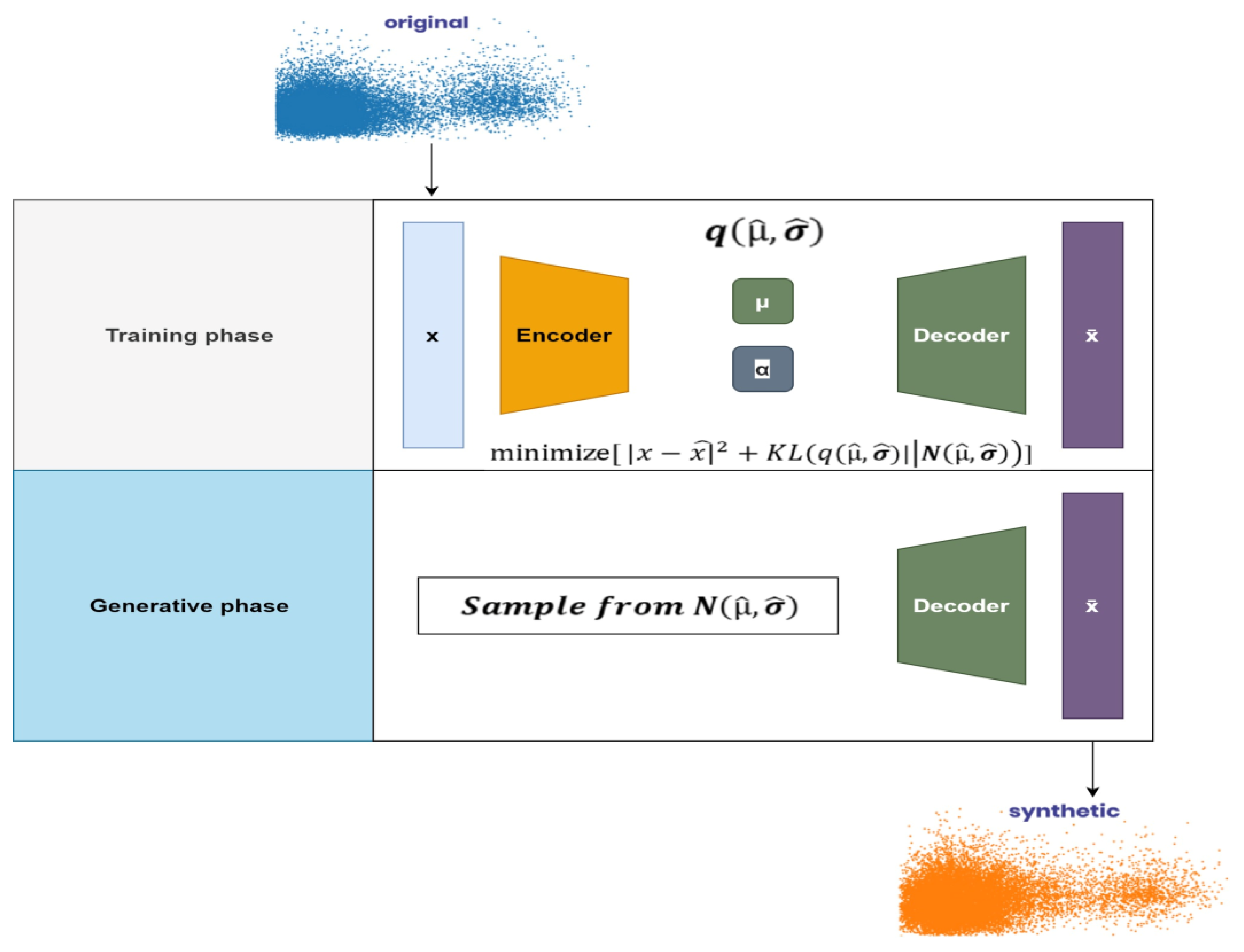
1.1. Variational Autoencoders

Variational autoencoders (VAEs) are creative models for probabilistic data comprehension. These autoencoders can learn the probability distribution of input data and create new data points that match the training data. VAEs use auto-encoders and probabilistic models for unsupervised data generation and dimensionality reduction. These methods are used in image, audio, natural language processing, and data compression [15,16]. VAEs train latent data representations through variational inference, which is their main novelty. This requires optimizing an objective function that balances autoencoder reconstruction error with a regularization term to achieve a desirable probability distribution for the latent representation. The regularization term is usually chosen to be a normal distribution, which allows for efficient sampling of the latent space and generation of new data points. The VAE intends to optimize the following loss function:

L = reconstruction_loss + KL_divergence_loss

where L shows the overall loss to be minimized during training of VAE, reconstruction loss evaluates the variance among the input data, and KL divergence loss assesses the distinction between the distributions across the latent representation, as the predetermined prior distribution.

1.2. Data Synthesis

Data synthesis or data augmentation is a common machine learning method for producing new training data from existing datasets. This method improves model resilience by adding non-training data variability. Classifiers perform better when sampling data class feature spaces. In domains where data is scarce, pattern recognition tasks can be particularly challenging due to limited variability in the available data, hindering the model’s ability to learn effective generalization [17]. Data augmentation can be used to add changes to training data while keeping labels to solve this classification problem. This can increase guidance class variance and restore model generalization. It includes combining data from several sources using statistical or computational approaches to find patterns, correlations, and trends that may not be visible from individual datasets. Data synthesis can transcend the limitations of individual studies by combining data from multiple studies to form a complete picture.

1.3. Forward Feature Selection

Feature selection (FS) plays a vital role in supervised learning tasks by identifying pertinent features that exhibit strong correlations with the target variable, while simultaneously removing redundant ones. This crucial process helps reduce computational burdens and improve the accuracy of results. By eliminating redundant features, the selection process ensures a more efficient and effective analysis. In this research, forward feature selection is employed to pick a subset of inputs and eliminate redundant attributes. The process of forward feature selection commences with an initial empty set of features and progressively incorporates the most crucial ones. A preset criterion, such as the strongest association with target variables or the lowest statistical test p-values, guides this. This continues until max features or model performances are met. The majority of synthesized datasets had imbalanced data; hence, this study used stratified cross-validation [18,19]. This paper contains the following notable characteristics and contributions:

• Introduction of variational autoencoders VAE for generation of synthetic data for transmission lines fault classification and localization that can improve the classification accuracy better than traditional methods.
• The technique is cost-effective and practical since it eliminates the requirement for a large volume of labeled real-world data.
• Demonstrates the capacity to detect faults in real-time and respond quickly, which can reduce the likelihood of power outages and improve grid dependability.
• Highlights the system’s ability to save time and effort by reducing the frequency of human monitoring and intervention.
• Tuned proposed machine learning architectures for greater accuracy compared to standard methods.
• Shows how machine learning techniques using enhanced synthetic data can accurately classify power transmission network issues.
• Research publications with scientific information contain limitations due to their design, methodology, and context.
• Predictions may be distorted by selected data points due to selection bias and the generated dataset must have 5000 data points to produce acceptable results.
• The proposed architectures require feature selection and hyperparameter adjustment and measurement errors also impact algorithm performance and lead to dataset inaccuracies.

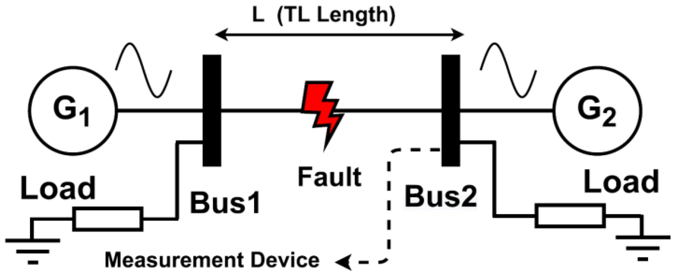
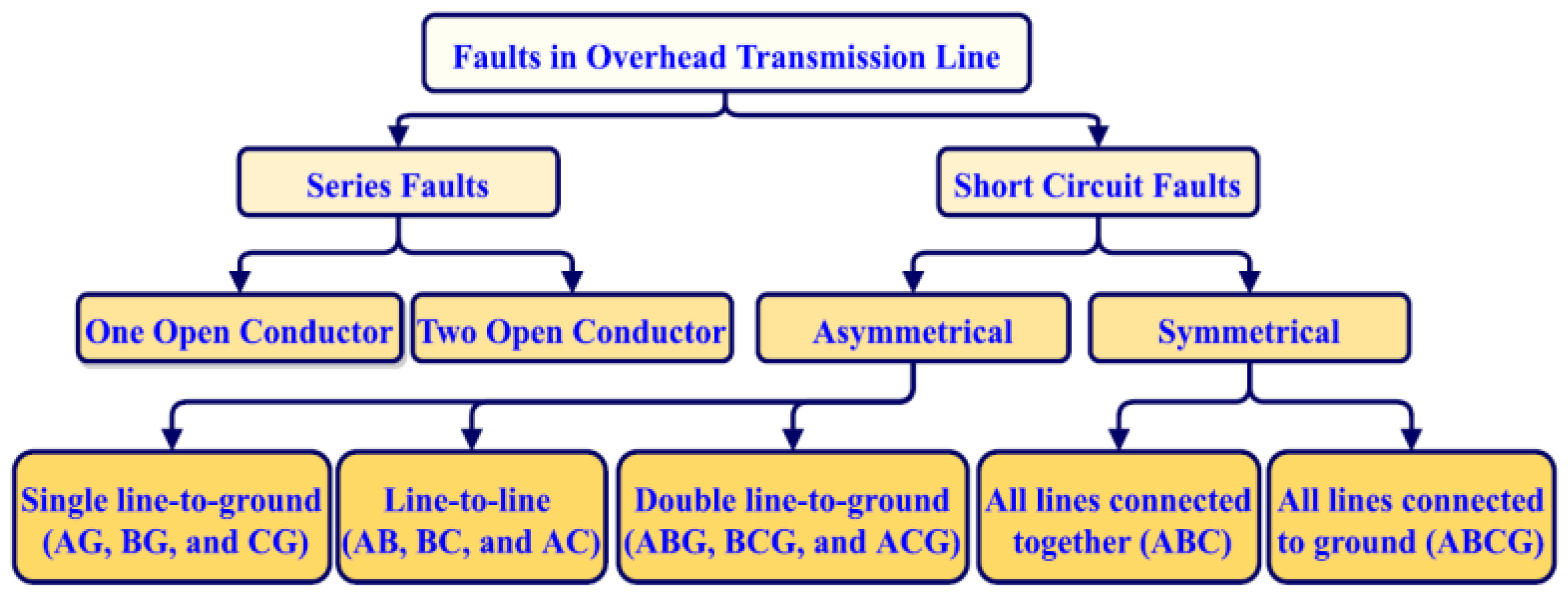
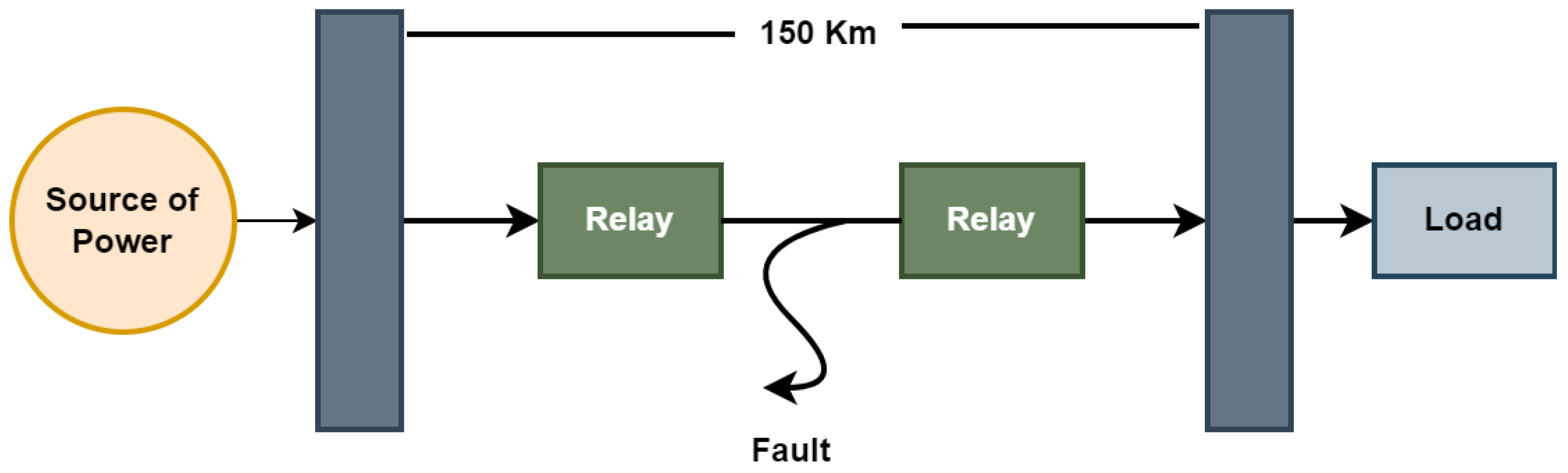
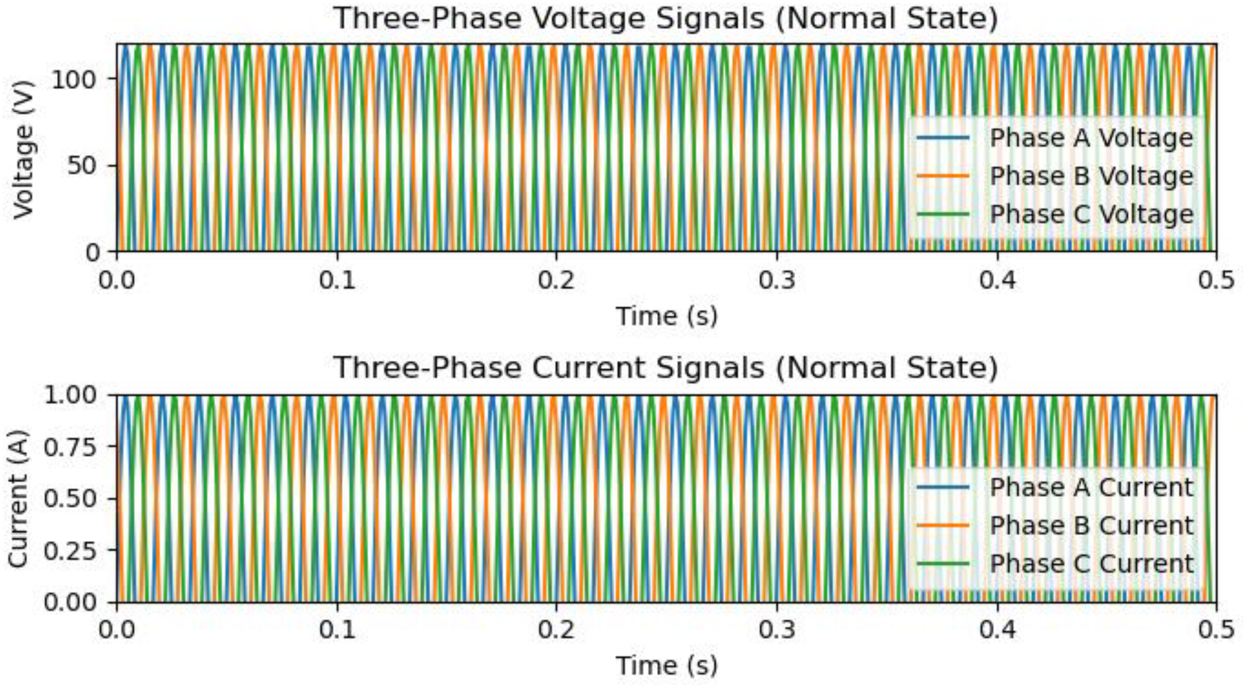
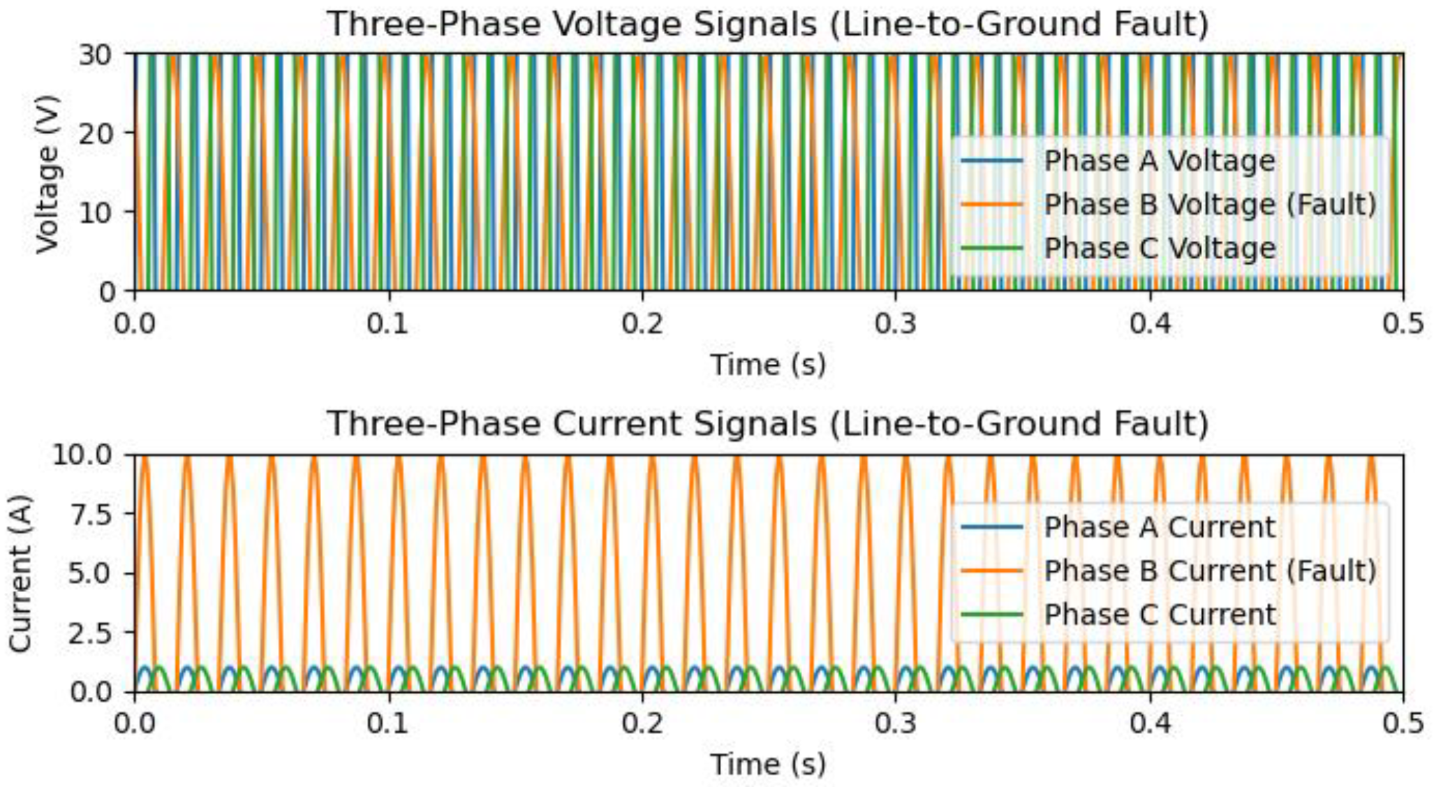
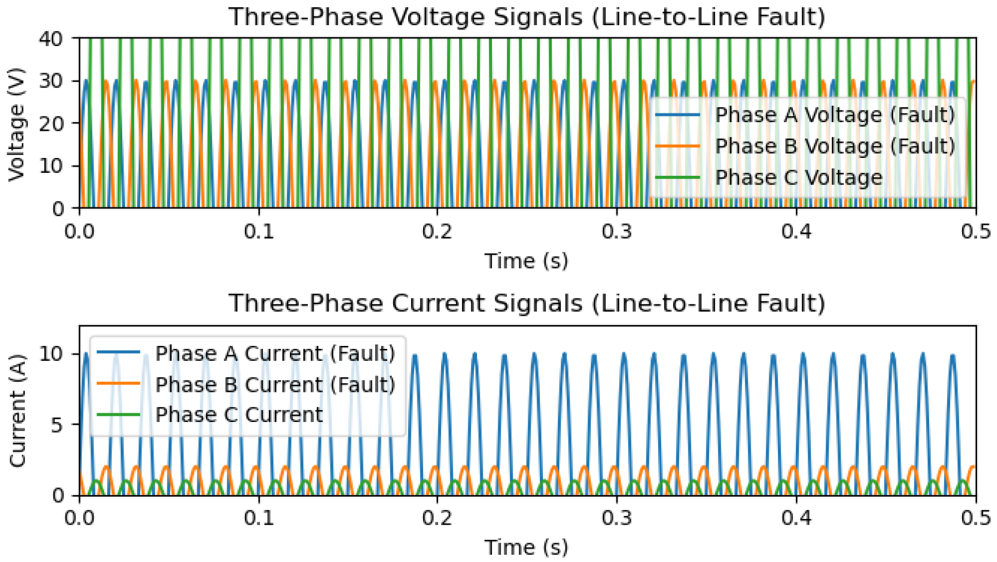
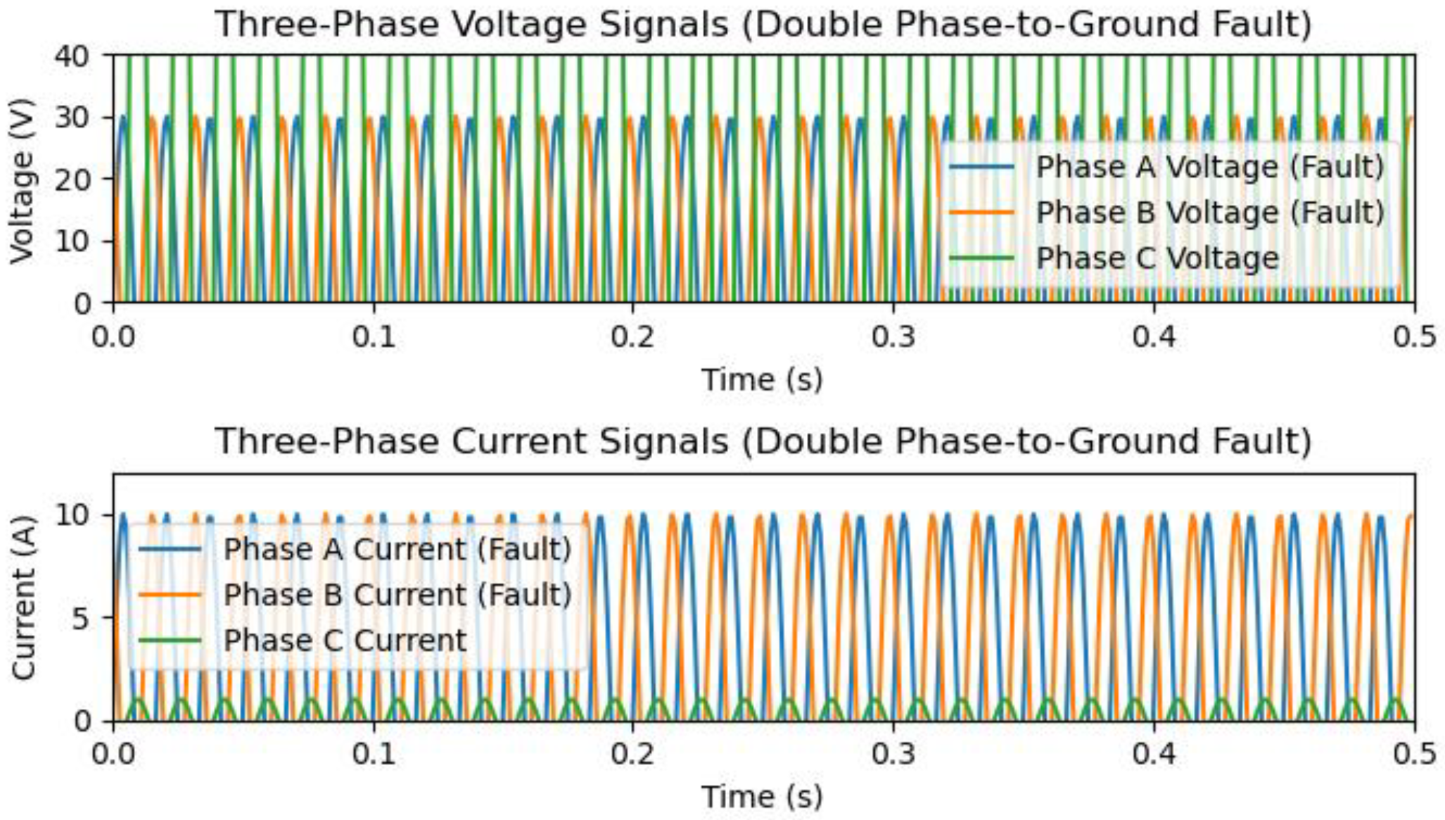
2. Modeling of 220 KV Transmission Networks

Modern power systems depend on transmission lines to accurately transmit electricity across vast distances with minimal losses. Abnormal transmission network conditions are infrequent, making incorrect data capture nearly impossible. Aspen one-liner, a powerful simulation tool used in industrial applications, is used to acquire datasets for practical training in all ML and DL architectures [20]. VAE variational autoencoders are used to construct and expand samples of all T/L shunt faults to improve power analysis for fault identification, categorization, and regression. In

Table 2. System components parameters for the proposed transmission network model.

Parameter	Unit	Value
Phase to phase (voltages)	KV	220
Source resistance (Rs)	Ohms (Ω)	0.7896
Source inductance (Ls)	Henry (H)	13.43 × 10−2
Fault incipient angle (φ)	Degrees	0° and −30°
Fault resistance (Ron)	Ohms (Ω)	0.001
Ground resistance (Rg)	Ohms (Ω)	0.01
Snubber resistance (Rsn)	Ohms (Ω)	0.9 × 10−4
Fault capacitance (Cs)	Farad (F)	infinite
Switching time	Seconds	b/w 0.1 and 0.2

and

Table 3. Sequence parameters for the proposed transmission network model.

Sequence Parameters	Unit	Value
Positive and negative sequence resistances (R1 and R2)	Ohms/Km	0.01154
Zero sequence resistance (Ro)	Ohms/Km	0.3165
Positive and negative sequence capacitance (C1, C2, and C3)	nF/Km	10.14
Zero sequence capacitance (Co)	nF/Km	5.7853
Positive and negative sequence inductances (L1, L2, and L3)	mH/KM	0.7945
Zero sequence capacitance (Lo)	mH/KM	2.9981

, transmission network parameters for their generation are provided. The line-to-ground (AG, BG, and CG), line-to-line (AB, BC, and AC), double line-to-ground (AB-G, BC-G, and AC-G), and three-phase-to-ground faults were created using this concept. This paper calculates parameters using the 220 KV three-phase transmission network model in Figure 4.

Data Preparation and Extraction

It is very crucial to extract real-world data in their original form, particularly in the context of modeling 220 KV power transmission networks. In our case, faulty data are extracted from the Aspen one-liner simulation tool to ensure that the information is correct and effectively utilized for modeling, analysis, and further research in this era. Voltage and current waveforms are employed to take out useful information and validate the occurrence of abnormal conditions on power transmission networks through machine language. Figure 5 shows the standard waveforms for voltage and current signals in the healthy state.

Under healthy conditions, waveforms of voltage and currents are in purely sinusoidal forms and have no distortion or noise, and the presented resultant waveform is standard. Power transmission networks experience extremely abnormal current flow and gradually drop the voltage to zero when an abnormal condition occurs. Figure 6 shows the single phase-to-ground fault and due to this, the voltage and currents of phases (A–C) are distorted due to abnormal instances on the line. The switching moment of the abnormal conditions is set between 0.1 and 0.2 and the location of fault is 132 km along the transmission networks.

Similarly, Figure 7 and Figure 8 show the line-to-line fault and dual-phase to-ground fault waveforms where, Ia, Ib, Ic, and Va, Vb, Vc, show sudden degradation in their magnitude. From these given circumstances, fault current and voltages are generated through machine languages which are further enlarged by variational autoencoders VAE to generate training datasets for classification and localization on power transmission networks. Figure 5, Figure 6, Figure 7 and Figure 8 illustrate the scenarios of a healthy state, single phase-to-ground fault, double phase-to-ground fault, and three-phase-to-ground faults generated from machine language.

3. The Use of Cat-Boost Architecture for Fault Classification and Localization

Yandex developers built Cat-Boost architecture to automatically handle crucial aspects and suggested model 2017 [21]. It adds priors to target its victim using variable statistics and combines category features to expand the dataset. It also trains practical datasets for transmission network abnormality classification and localization using machine language. It outperforms PCA, SVM, and ANN because it automatically handles categorical features to improve classification and regression. Cat-Boost does not require feature-to-number conversion or pre-processing for numerous fault categories. Cat-Boost minimized hyperparameter modification and used binary Decision Trees as basis predictors to solve complex, noisy, and hydrogenous problems [22]. It loads all sample datasets into the training architecture, mixes a GBDT with unconditional features, and transforms each sample’s x-tics before sampling for calculation. Using a sample size for data:

D = {(Xj, Yi)}; j = 1.

Based on a vector of n characteristics (Xj = Xj1, Xj2, …, Xjn) and a binary value (0, 1), the sample (Xj, Yi) is distributed uniformly and independently by an unknown distribution P(.,.). The function trains H: Rn→R to minimize the anticipated loss in the equation:

L (H) = EL(y, H(x))

where L stands for plane function and (X, Y) is the test dataset from training dataset D. Sampling all data points for training in Cat-Boost architecture increases model resilience. When changing each data point’s x-tics, the desired value is sampled and then assigned relative weights. Cat-Boost requires minimal data training and accepts missed statistics and non-coded integer attributes.

Dataset Training Employing Cat-Boost Architecture

About 18898 data points are generated for the mentioned diverse kinds of abnormal conditions, including healthy state, line-to-ground, line-to-line, double line-to-ground, and three-phase-to-ground faults. Data points are split into training for 70% and testing for 30%, respectively. Cat-Boost architecture is implemented as a machine language on the dataset for practical training and it can handle categorical features automatically for excellent classification and regression results. The input data to the proposed architecture are three-phase current and voltage data points, and their optimization parameters are listed in

Table 4. Optimization parameters for Cat-Boost.

Hyperparameter	Description	Value
Iterations	No. of boosting iterations	1000
Depth	Depth of the tree	6
Learning rate	Learning rate	0.1
Loss function	LS for classification/regression	Log loss/RMSE
Class weight	List of categorical features	0.01, 0.001, 0.9, 0.0001
Verbose	Print progress every X iterations
Random strength	Search randomly a certain number of combinations	0.1

. The suggested technique is superior to other machine learning models which have longer training time and demand high computational cost. The optimized parameters for the Cat-Boost algorithm are selected carefully through the tuning process for admirable outcomes.

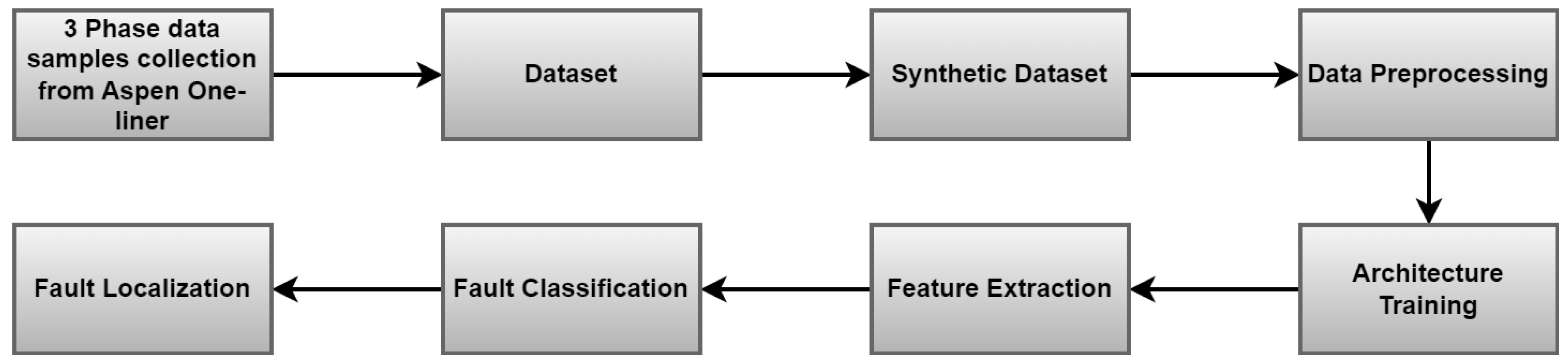
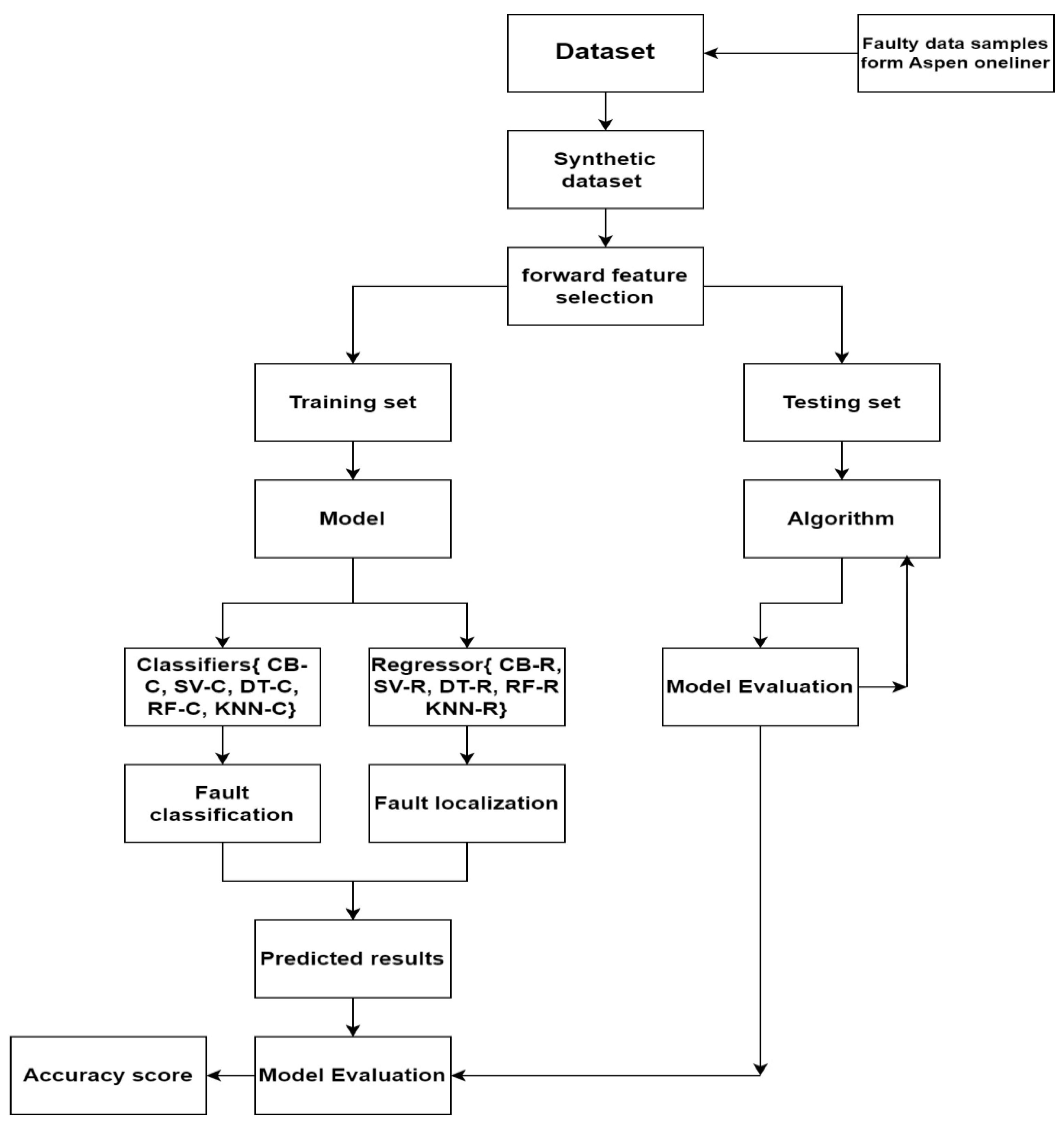
4. Proposed Methodology

A lot of data is needed to develop good models for many machine-learning applications. Synthetic datasets are too important to generate when real-world data is scarce. Machine learning and deep learning algorithms can create synthetic data from existing datasets to guide ML architecture. The datasets train the model for fault classification and transmission line localization. The datasets with no missing values are considered as ideal. Datasets train machine learning models. Classifying faults requires these ML models. After training the ML model, testing is carried out on the ML model to check the accuracy models. Figure 9 shows the proposed methodology for the classification and regression of abnormal circumstances in transmission-carrying networks. SVMs are useful for fault classification and localization, assisted by supervision to find the hyperplane for separating data point types [23]. They may considerably improve fault classification and localization processes to find the best hyperplane in n dimensions [24,25].

Define a maximum tree depth to minimize overfitting in Decision Tree classifiers that employ information gain and Gini index scoring algorithms. The system adjusts depth to balance generalization and training set performance [26]. Gini index, entropy, and CART determination analyze points [27,28]. Random Forest divides the dataset into training data (the “in bag” data) and validation data (the “out of the bag” data) to detect power system problem characteristics [29,30]. This unpredictability diversifies ensemble trees and improves algorithm performance [31,32]. KNN improves power transmission system fault management by detecting and categorizing defects [33]. Euclidean, Manhattan, and Mahalanobis distances are used to improve the K-Nearest Neighbors (KNN) method [34,35]. Approximate KNN approaches use indexing structures like KD-trees and Hash tables to reduce the search space and improve computing performance, especially for big, unbalanced datasets.

5. The Process of Data Generation and Simulation for T/L with Aspen One-Liner

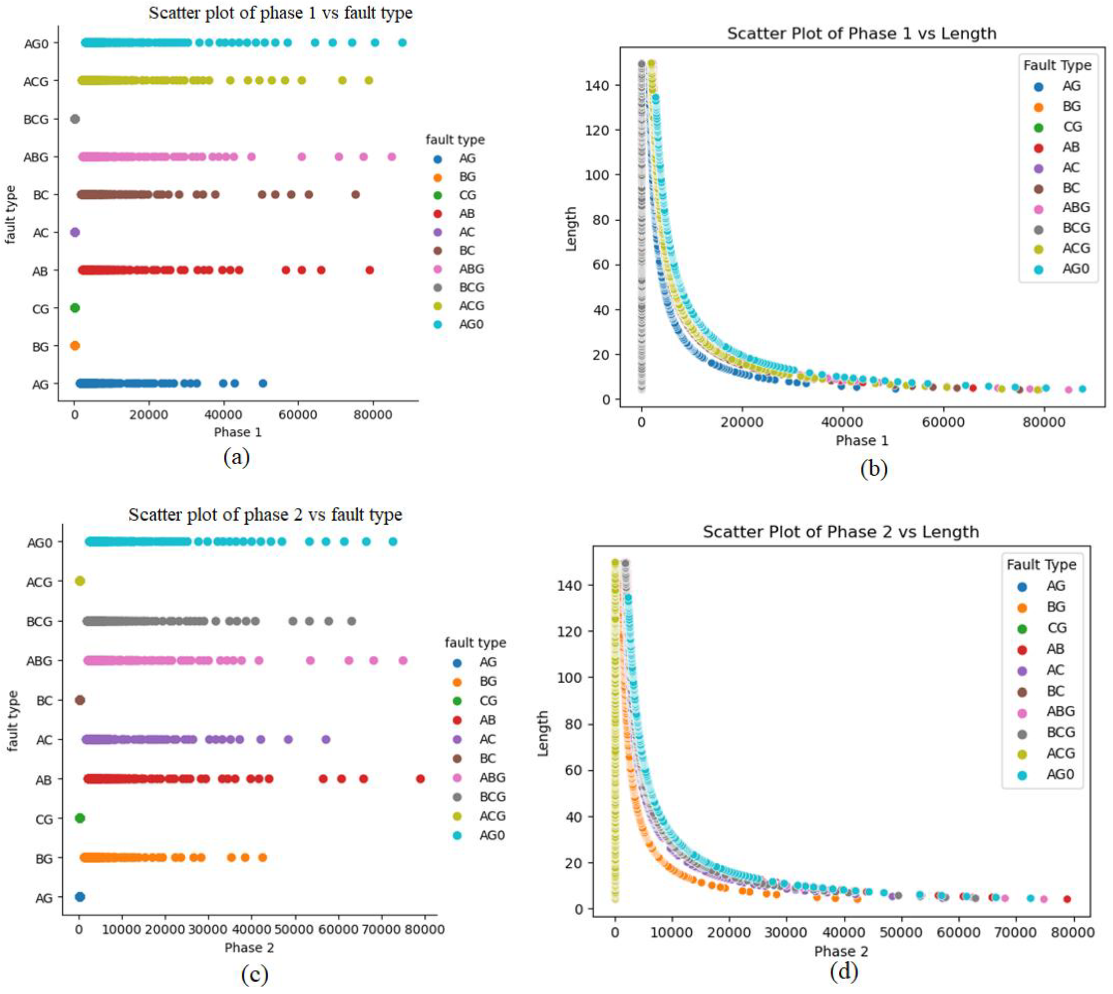
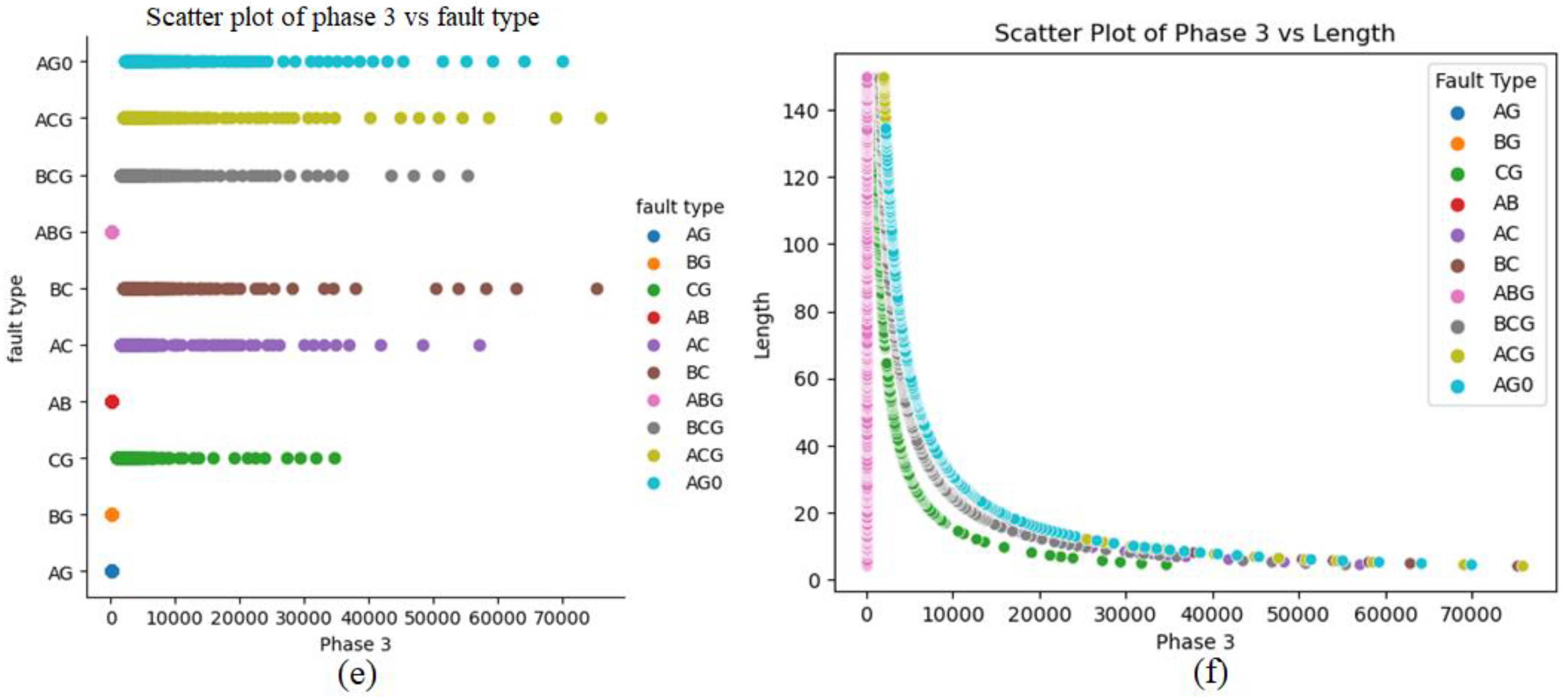
The proposed methodology involves the utilization of experimental platforms encompassing both two-terminal and three-terminal transmission networks. The assessment of these transmission models entails the application of Aspen one-liner, a productivity-enhancing tool geared toward analyzing and modeling transmission and distribution networks. This software effectively compiles replicated data by simulating diverse transmission network defects under varying operational conditions, facilitating the export of relay testing fault data. During instances of transmission network malfunction, post-fault voltages in all three phases (Va, Vb, and Vc) along with the ground mode are meticulously recorded for a single cycle at each terminal. In pursuit of generating real-time datasets, fault levels are manipulated by introducing alterations in various transmission network fault conditions across multiple locations. This real-time dataset is then employed to enhance the original dataset, resulting in the creation of a synthetic dataset.

Table 5. Fault sample information.

Fault Type	Fault Label
Line-to-ground	AG
Line-to-ground	BG
Line-to-ground	CG
Double line-to-ground faults	ABG
Double line-to-ground faults	BCG
Double line-to-ground faults	ACG
Line-to-line faults	AB
Line-to-line faults	BC
Line-to-line faults	AC
Three line-to-ground faults	ABC-G

presents comprehensive data sample information about a range of shunt faults that have occurred on both the two-terminal and three-terminal transmission lines. Applying variational encoders (VAEs) to the list of defects within Table 5 yields a total of 2183 synthetic samples, further enriching the dataset.

VAEs are talented algorithms that can create synthetic data for double and triple power transmission networks for abnormal condition classification and localization. This novel method uses Aspen one-liner data samples to construct a new dataset. VAEs, a sort of generative model, may encode input data into a compact latent space and decode it to generate novel data samples that closely match the original data distribution as shown in Figure 10. This strategy has shown promise in several applications, including resolving imbalanced class distributions by using synthetic examples [36]. Generating a synthetic dataset from the original dataset is extremely beneficial in critical situations where the existing dataset is small and imbalanced, and we want to generate some additional data to get better recital of the ML model. After generating some samples of shunt faults for transmission networks, variational encoders (VAEs) are employed to enlarge this synthetically. Real-time fault recorders are used for recording real-time faulty samples for transmission networks [37,38].

They also duplicate the patterns present in the initial dataset by employing encoder and decoder functions. These functions transform the original dataset into a smaller version, effectively creating an expanded synthetic version. These datasets include information, such as phase voltages, location details, and various examples of shunt faults found in transmission networks. These artificially generated data are utilized to teach the ML architectures and assess the effectiveness of the designs [39,40]. For three-terminal networks, only two samples are taken as faulty samples for each fault type and similarly, for two-terminal networks, one faulty sample is considered as faulty. Attributes of training and testing datasets are shown in

Table 6. Attributes of training and testing datasets.

Attributes	Training Dataset	Testing Dataset
Fault types	All kinds of shunt faults	All kinds of shunt faults
Fault resistances	0, 25, 50, 75, 100, 150	0, 25, 50, 75, 100, 150
Fault distances	Increments of 4.4 km to 150 km	Increments of 4.4 km to 150 km
Size	14,400	4498

, while all types of shunt faults as mentioned in

Table 7. Optimum parameters for proposed architectures.

Hyper-Tuning Parameters for SVM		Hyper-Tuning Parameters for DT
Tuning parameters	Values	Parameters	Values
Kernel function	linear	Criterion	entropy
Regularization parameter (C)	0.1	Splitter	best
Kernel Coefficient (gamma)	0.1	max_depth	90
Coefficient of kernel	1	min_samples_split	3
Validation accuracy	1	min_samples_leaf	2
		max_features	5
		ccp_alpha	0.01
Hyper-Tuning Parameters for Random Forest		Hyper-Tuning Parameters for KNN
Parameters	Values	Parameters	Values
Criterion	entropy	n_neighbors	3
Splitter	best	weights	distance
max_depth	90	metric	Euclidean
min_samples_split	3
min_samples_leaf	2
max_features	5

are simulated at each value for both transmission networks. The fault classification accuracy and localization error of the given dataset by employing machine learning algorithms are 99.13% and <2%, respectively.

Data Splitting

The dataset includes two essential sets: (a) the training set, and (b) the evaluation set. In the domain of ML algorithms, the process of dividing action datasets into training and testing sets holds great importance. In our suggested approach, the dataset has been partitioned, allocating 70% for training purposes and 30% for testing. After the algorithm has been trained, the model’s effectiveness will be assessed by examining its performance on the testing data.

6. Performance Evaluation and Comparative Analysis

This section aims to provide a concise overview of the synthetic dataset, highlighting its connections to various types of shunt incidents occurring on transmission lines, along with their respective locations. Furthermore, we will introduce a comprehensive set of assessment metrics that effectively gauge the performance of both the classifier and regressor models. To visually portray the data distribution, we will adopt scatter plots, a technique that presents data points on a two-dimensional graph. This method serves as a robust tool for visualizing relationships and patterns embedded within the dataset. The utilization of scatter plots is intended to enhance the clarity and intuitive understanding of the dataset’s complexities, facilitating a deeper exploration of individual interactions and behaviors. Figure 11 provides the scatter plot information of every value present in the synthetically generated dataset through VAEs for classification and localization of faulty points of (a) phase 1, (b) phase 2, and (c) phase 3, respectively.

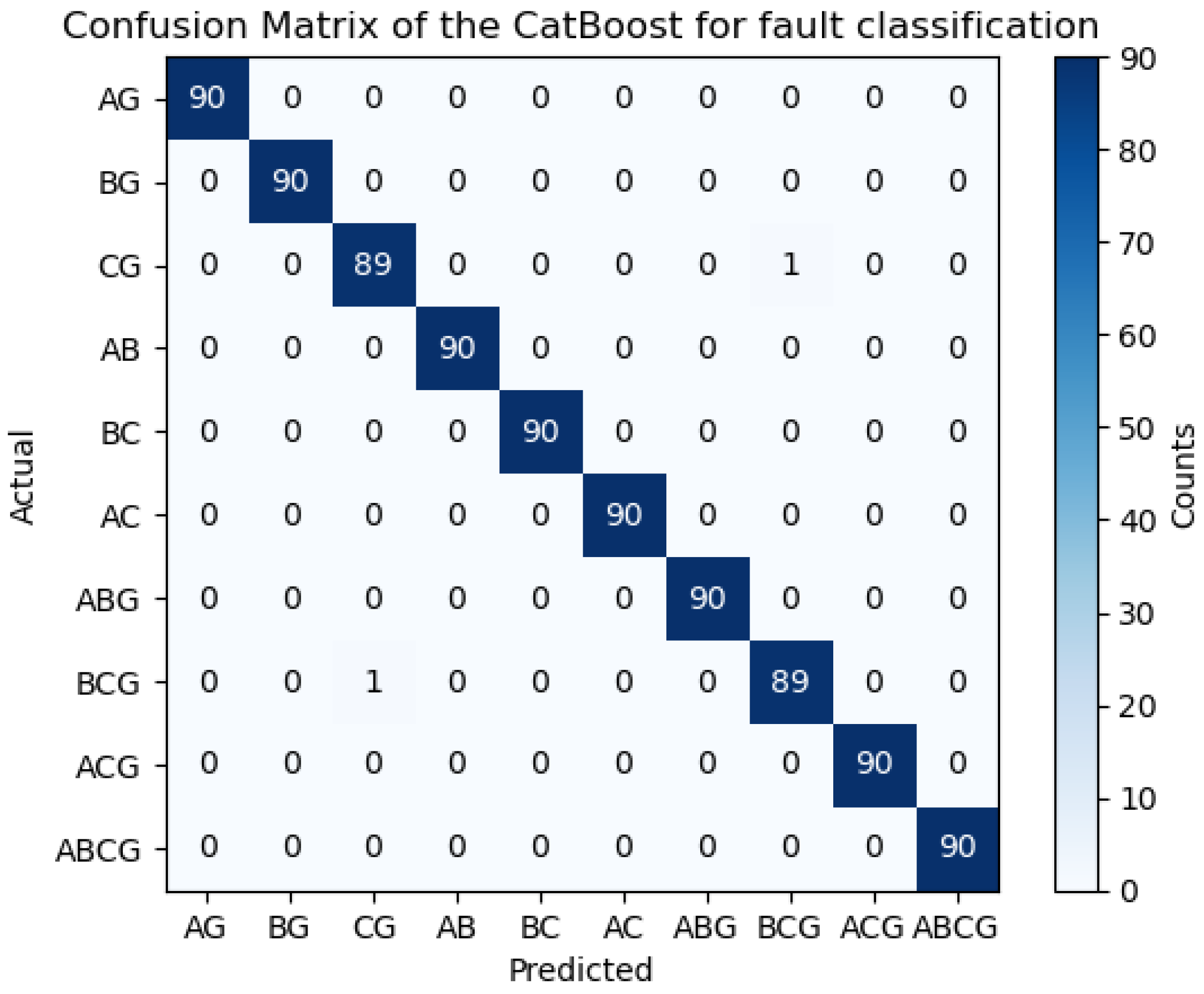
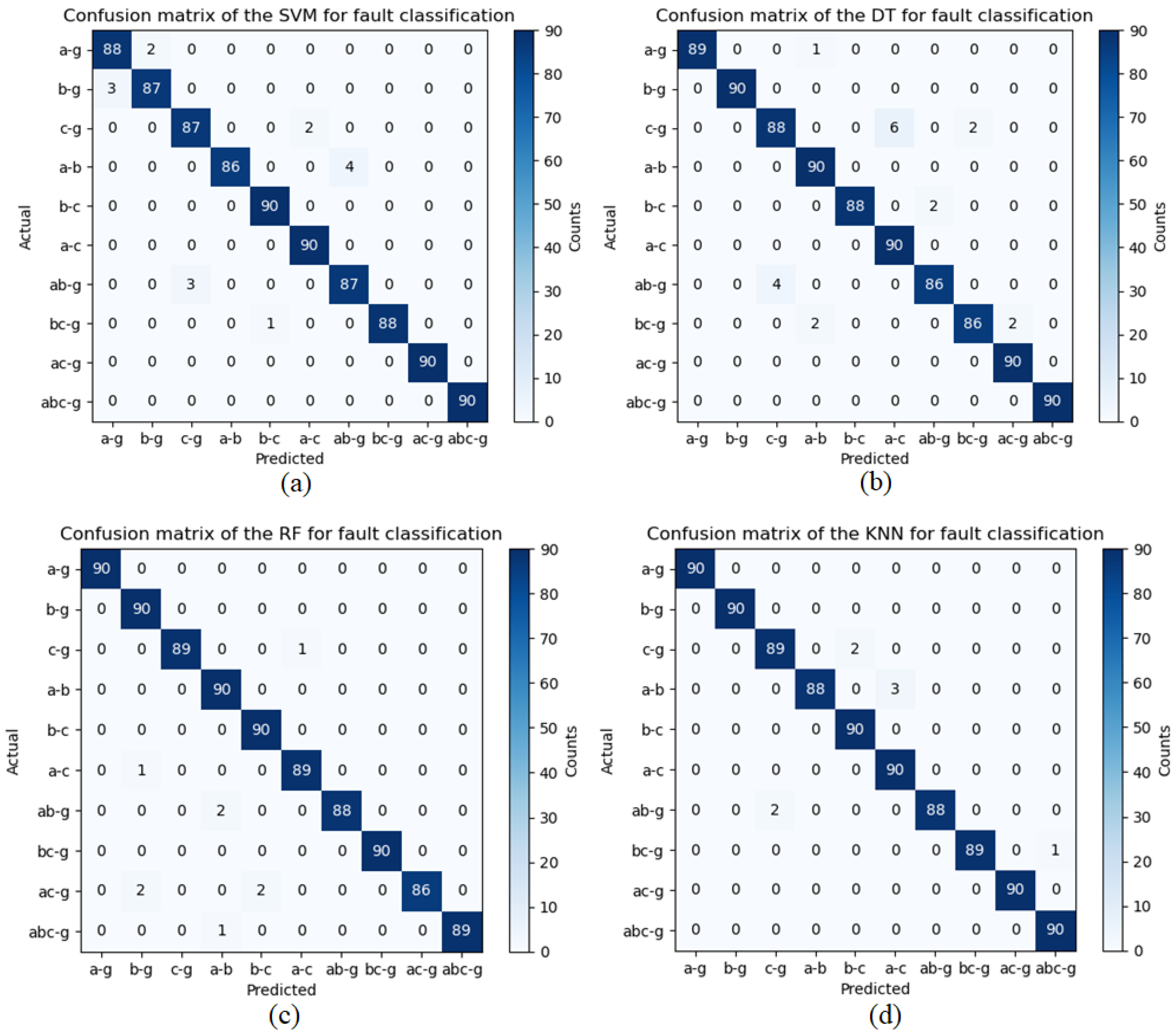
6.1. Confusion Matrixes for Predictive Modeling of Classification Algorithms

In this study, we employ a confusion matrix to assess various types of shunt faults, encompassing line-to-ground faults (AG, BG, and CG), line-to-line faults (AB, BC, and AC), double line-to-ground faults (ACG, BCG, and ABG), as well as three-phase faults (ABC-G). Four tentative scenarios are evaluated to measure the performance of the proposed ML algorithms based on accuracy for calculating the ratio of the correctly classified and unclassified abnormal circumstances against the total number of values. The accuracy is calculated as:

$$Accurcay=\frac{TP+TN}{TP+TN+FP+FN}$$

In the context of classification analysis, the acronyms TP (True Positive), TN (True Negative), FP (False Positive), and FN (False Negative) hold significant meaning. These descriptions result from a confusion matrix that presents a counter-process of the predictive performance of a classification model. Figure 12 shows the confusion matrix for the diagnosis of predicting outcomes based on proposed architectures for all kinds of shunt faults on power transfer networks. Similarly, ROC curves and regression outcomes obtained from Cat-Boost architecture are presented in Figure 13 and Figure 14, respectively.

6.2. Models Hyperparameters Tuning

Hyperparameter research was carried out to find the best settings for RFR and the other models to be compared with. To find the optimal hyperparameters, researchers can choose one of two routes: There are two types of searches: grid searches and random searches. Using a sample of the data, grid search was used to investigate the important parameters for each model and their optimal values. For KNN, we settled on uniform and distance weighting functions, each with different numbers of neighbors. In SVM, both polynomial and radial basis function (RBF) kernels were selected. In addition, we looked at several different values for the regularization parameter C. The lowest number of samples required to divide a node internally in DT was found, and various values were examined to regulate unpredictability inside the tree. Alpha and lambda were chosen as the shape parameters for DT. Alpha represents the gamma distribution before alpha, while lambda represents the distribution before lambda. To find the appropriate split, the RFR technique used two maximum feature methods, sqrt, and log2, to calculate the number of characteristics to evaluate [41,42]. The best parameters for each model are highlighted. Table 7 shows the optimal hyperparameter through a hyperparameter search for appropriate values to enhance the accuracy of the training model of the SVM for the proposed methodology.

To calculate the classification truth of shunt faults, the dataset is separated into training and testing subsets, with 70% of the data allocated for training and the remaining 30% for testing. The confusion matrix offers valuable insights into classification precision, where the diagonal elements signify accurately predicted cases, and the off-diagonal values represent misclassifications. Figure 15 illustrates the visual representations of the confusion matrices for (a) SVM, (b) DT, (c) RF, and (d) KNN to diagnose shunt faults on power transfer networks.

The confusion matrix is employed to visualize the numeric test results, including true positives, true negatives, false positives, and false negatives, highlighting the effectiveness of the machine learning classifier [43]. In this matrix, the diagonal values represent accurately classified instances, while the non-diagonal values correspond to unclassified instances in the fault classification task for power transmission lines.

Table 8. Testing outcomes of fault classification employing suggested ML learning algorithms.

Machine Learning Model	Fault Types	No. of Test Data Samples	Accurately Classified Samples	Misclassified Samples	Accuracy %
SVM	LG (a-g, b-g, c-g)	270	268	2	99.25
	LL (a-b, b-c, c-a)	270	266	4	98.51
	LL-G (ab-g, bc-g, ac-g)	270	266	4	98.51
	LLL (abc)	90	90	0	100
DT	LG (a-g, b-g, c-g)	270	261	9	96.66
	LL (a-b, b-c, c-a)	270	268	2	97.74
	LL-G (ab-g, bc-g, ac-g)	270	262	8	98.95
	LLL (abc)	90	90	0	100
RF	LG (a-g, b-g, c-g)	270	269	1	99.62
	LL (a-b, b-c, c-a)	270	269	1	99.62
	LL-G (ab-g, bc-g, ac-g)	270	267	3	98.88
	LLL (abc)	90	89	1	99.62
KNN	LG (a-g, b-g, c-g)	270	269	1	99.62
	LL (a-b, b-c, c-a)	270	269	1	99.62
	LL-G (ab-g, bc-g, ac-g)	270	267	3	98.88
	LLL (abc)	90	90	0	100

presents the fault classification results for the proposed machine learning algorithms, namely SVM, DT, RF, and KNN, as utilized in this study. It also demonstrates that the classification results for shunt defects that occurred on power transmission lines using the ML algorithms proposed in this article are of extremely high accuracy of up to (99.50%).

6.3. Performance Evaluation Parameters for Classification Models

There are various methods to evaluate the efficiency of classification architectures, which rely on the attributes of the test dataset. These methods include recognized measures, such as precision, accuracy, recall, and F1 score, derived from the confusion matrix analysis. These evaluation parameters are computed based on the elements of the confusion matrix plot, tailored to the specific domain of the problem, and offer a thorough understanding of the analysis. The outcomes of these assessment metrics are demonstrated in

Table 9. Performance evaluation parameters for classification models.

Classifier	Accuracy	Precision	Recall	F1 Score
SVM	0.99	0.99	0.99	0.98
DT	0.97	0.98	0.97	0.98
RF	0.99	0.99	0.99	0.99
KNN	0.98	0.99	0.97	0.98

, presenting the results of the classification models in terms of their assessment measures.

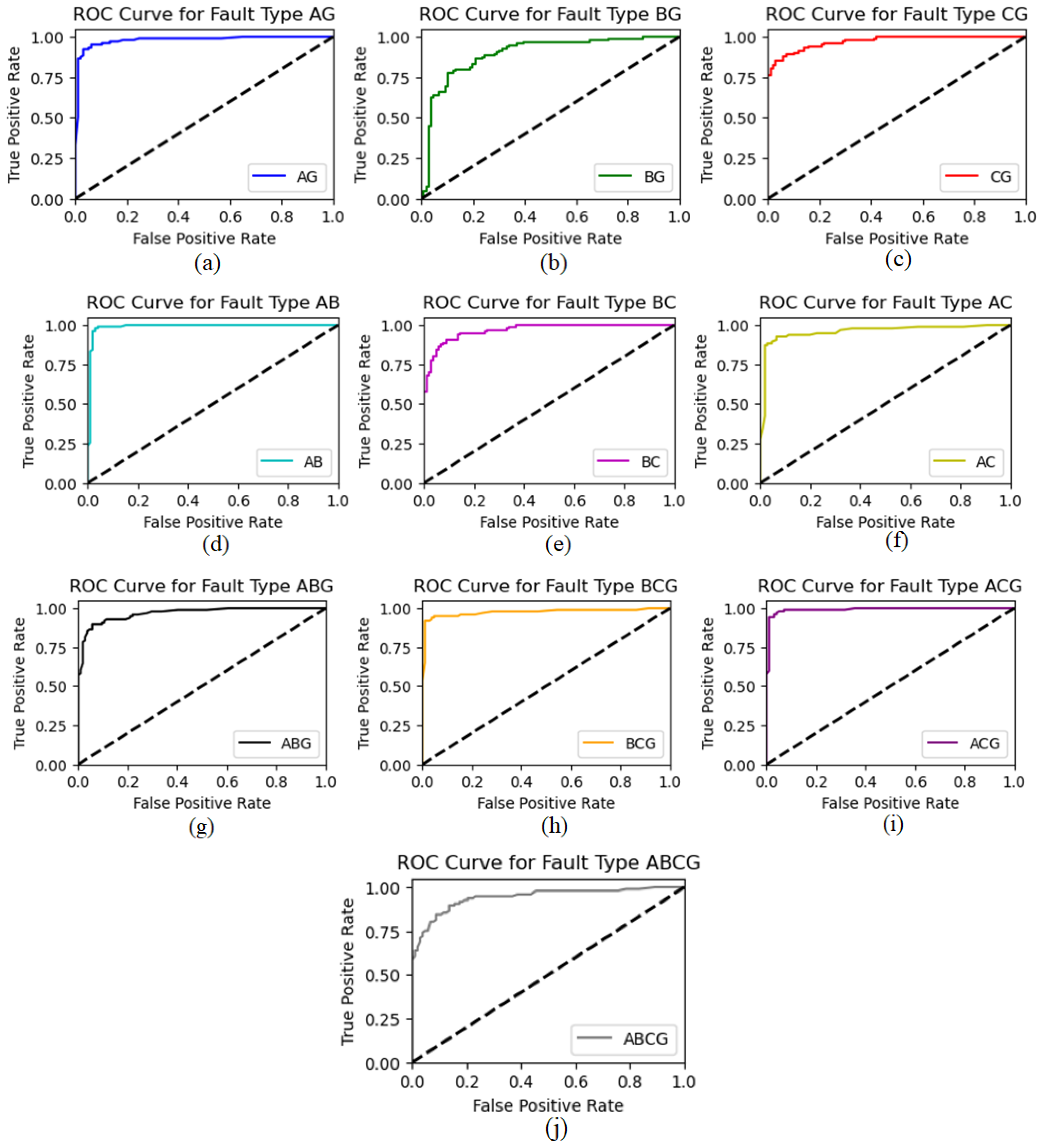
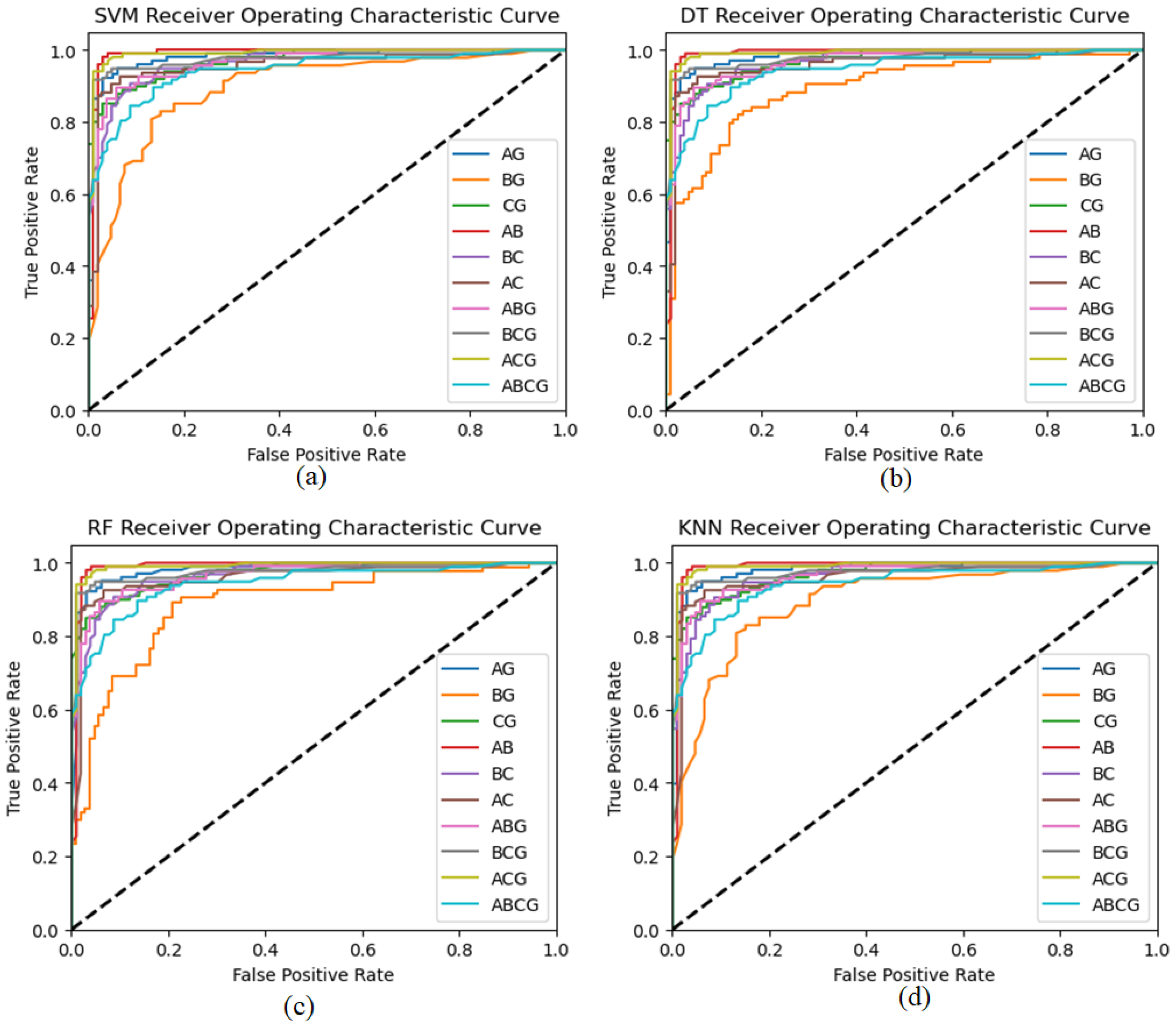
6.4. Receiver Operating Characteristic (ROC) Analysis for Proposed Architectures

ROC curves assess classification models and show the model’s classification efficiency when thresholds change through the ability to distinguish classes by balancing sensitivity and specificity. Four classifiers—SVM, Decision Tree, Random Forest, and KNN—were examined. We predicted class membership probability for the test dataset after training each classifier. These predicted probabilities generated ROC curves. FPR and TPR are on x and y. The random guessing ROC curve is a dashed black diagonal line. Classifiers hope curves over this diagonal outperform random chance. Starting with the SVM classifier (solid lines), we get fault-type-specific ROC curves with AUC values. Dashed Decision Tree classifier ROC curves capture complex decision boundaries. The Random Forest classifier (dotted lines) uses many Decision Trees to smooth fault-type curves [44]. ROC curves for the neighborhood-based K-Nearest Neighbor (KNN) classifier (dot lines). Dataset and neighbor count affect KNN performance. ROC curves reveal each classifier’s strengths and weaknesses. This helps us find fault-tolerant and multi-class models. We prioritize ROC curves and AUC values for classification model evaluation. These metrics help select a problem domain’s best classifier by assessing a model’s class discrimination. Figure 16 shows the ROC curves for SVM, DT, RF, and KNN to show the accuracies of classification results on the power transmission lines.

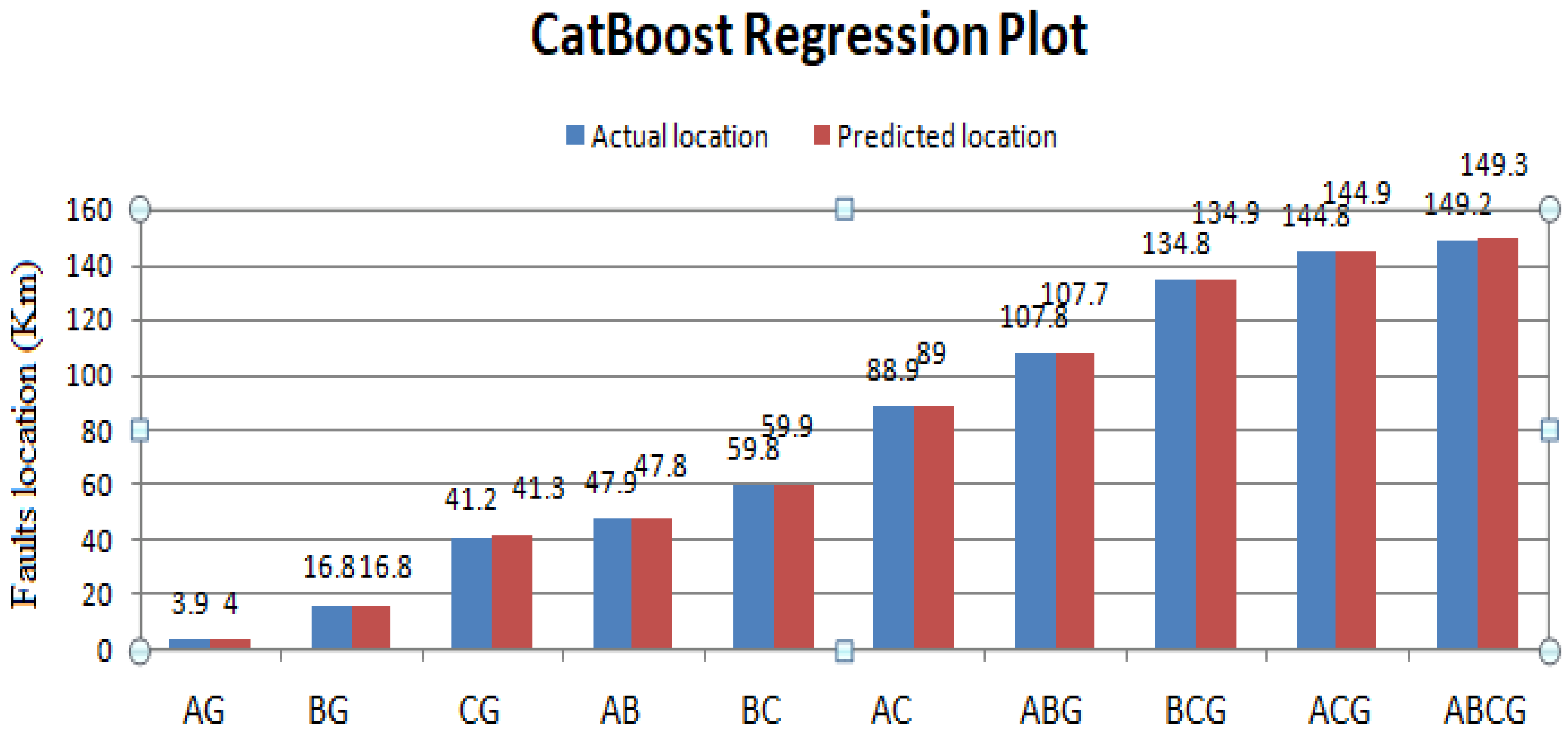
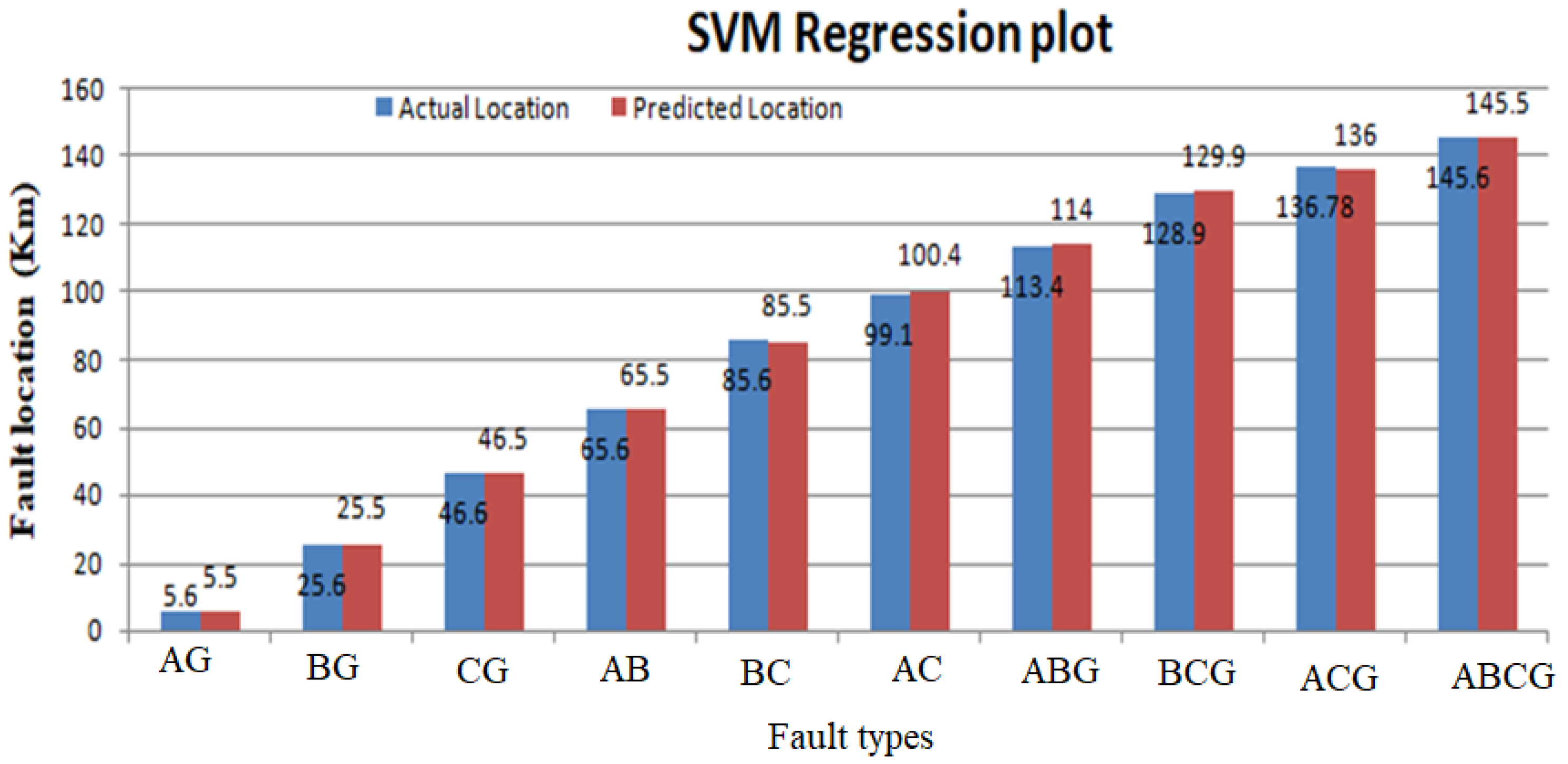
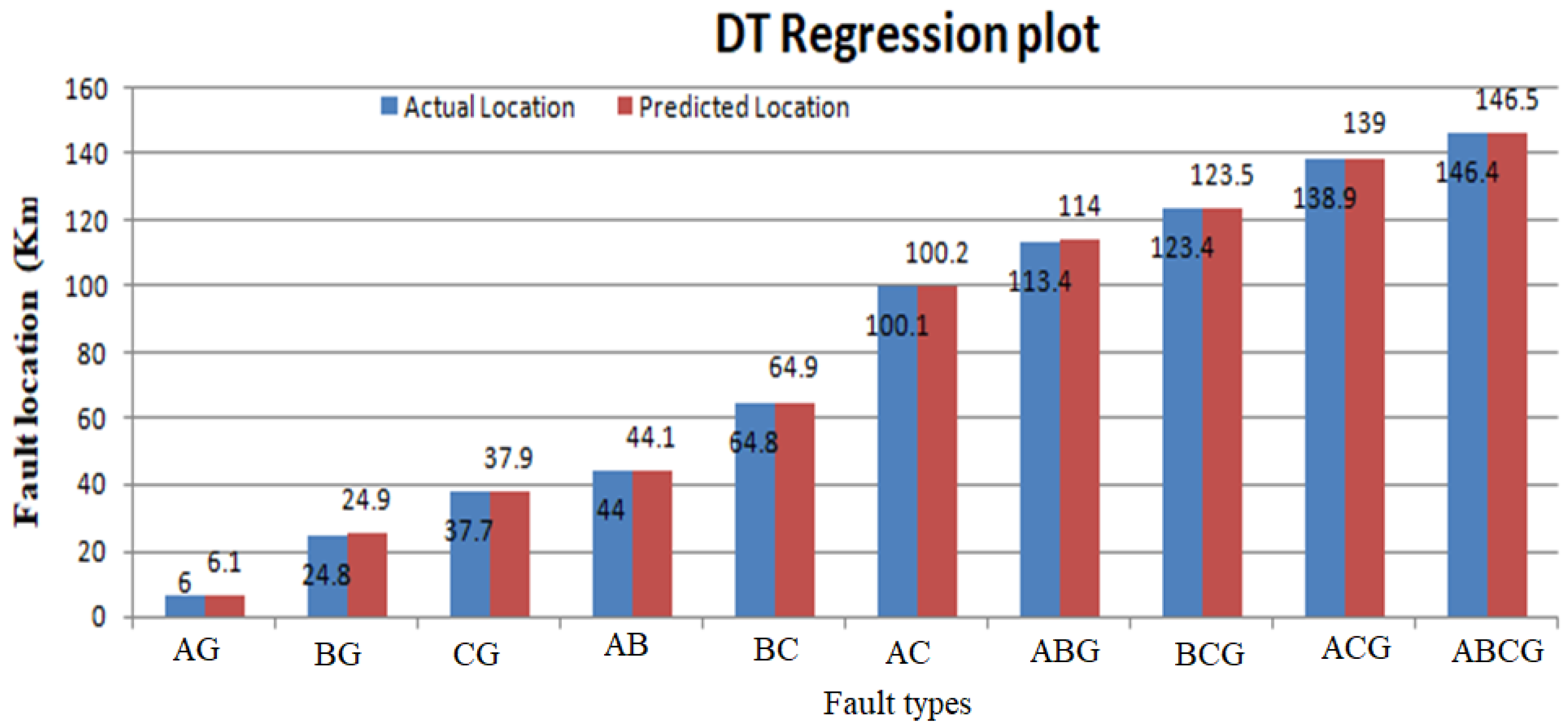
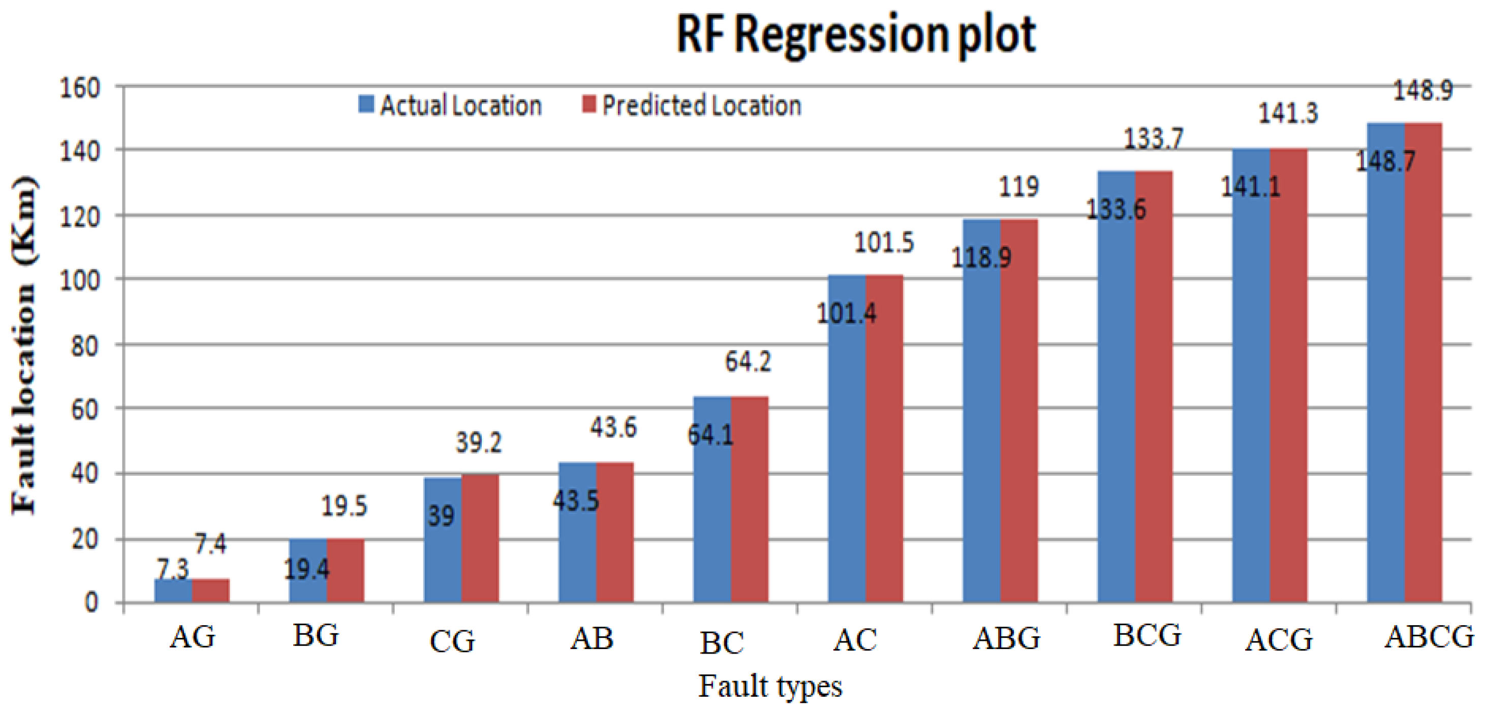
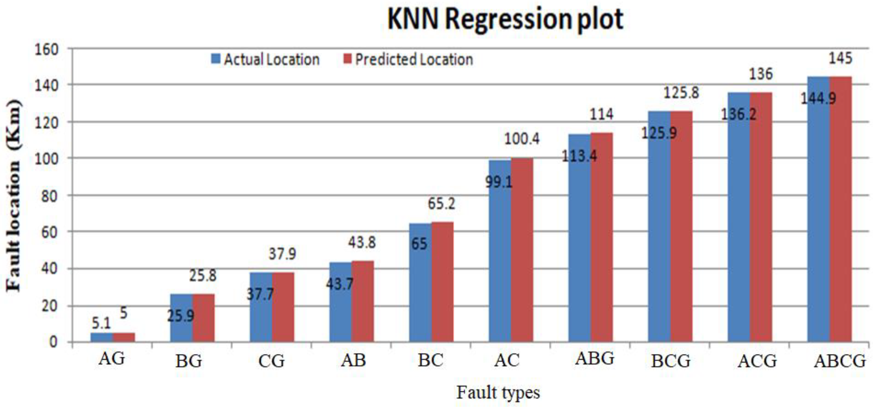
6.5. Fault Localization Results

Once a specific type of fault is identified through the proposed classifier architecture, the precise prediction of shunt fault locations within transmission networks is achieved using regression models. The primary objective of these regression models is to establish a functional mapping between the input features (independent variables) and the target variable (a continuous value). Furthermore, regression serves as a means to uncover the intricate relationship between continuous input variables and their corresponding output variables. In the capacity of a regressor, a selection of diverse machine learning algorithms comes into play to pinpoint power line faults. The process involves conducting regression computations for unforeseen data instances, accounting for both the proximity and distance of the ends under observation. The regression outcomes are delineated in Figure 17, Figure 18, Figure 19 and Figure 20, illustrating a comparative analysis between the actual fault locations and those forecast by the suggested ML algorithms (SVM, DT, RF, and KNN).

Table 10. Table for true and predicted values of fault localization and amount of error.

Machine Learning Model	True Fault Distance	Predicted Fault Distance	% of Error
SVM	116.9	115.6	1.3
	104.4	103.7	0.63
	52.4	51.5	0.9
	115.1	113.8	1.36
DT	21.6	21.2	0.4
	114.2	112.8	1.4
	74.4	73.3	0.7
	50.0	49.2	0.8
RF	61.2	59.7	1.5
	48.1	47.6	0.58
	103.3	102.4	0.92
	146.4	145.9	0.9
KNN	115.6	114.8	0.8
	104.4	103.9	0.48
	112.8	112.2	0.6
	21.2	20.2	0.99

presents the outcomes of the regression model for both real and predicted fault localization values. It also illustrates the extent of error experienced in power transfer lines due to the implementation of the suggested approach. The actual values are shown by a blue line as mentioned in the regression graph and the regression line is shown by the red dotted line. So, the regression line is linear, and the accuracy of the regression system predicted good results. The term absolute error is used to evaluate the regression results on the power lines. The absolute error gives the results of the actual length on which the fault occurred and predicted results, which are predicted by machine learning models. In absolute error, y-predicted is the value predicted by the machine learning model and y-true is the true fault distance. The absolute error is given as

$$Absolute error=|true fault distance-predictedfault distance|$$

7. Conclusions

This study demonstrates the different machine learning algorithms for the recognition of all types of shunt faults on transmission lines and their location tracing based on synthetic data instead of using traditional trade-off planning. Transmission networks are the most critical part of the power transfer system and are used to transfer power from one end to other far ends. Different protecting relaying systems are installed on the grid/substation for the sensitive operations of transients which mostly occur on the power system. When abnormal conditions occur, then it will be necessary to remove the faults within no time and restore the power to end-users. The collection of real data for making datasets is the major problem in implementing and training models. This study is based on the analysis of data obtained from simulations of transmission networks using Aspen one-liner, which is further expanded by employing variational encoders to enlarge it synthetically. Machine learning algorithms are the best solution for complex networks. These algorithms are easy to implement, and the best performance results can be obtained, restoring the power supply for a safe and reliable country’s energy system. The proposed methodology is simple to implement for the existing protection system. Machine learning models are trained by datasets and feature selection methods. In the classification process, the model is trained to classify the shunt faults, which mostly occur in the power system. Support Vector Machines, Decision Trees, Random Forests, and KNN models are used for classification and regression. All the classifiers provide admirable results for the classification and localization of faults on transmission networks. This research work also highlights the importance of data quantity, and increasing the amount of data synthetically for training improves the accuracy of architectures they also emphasize the need for accurate fault data labeling and feature selection to achieve optimal results.

References

1. Dinsdale, N.J.; Wiecha, P.R.; Delaney, M.; Reynolds, J.; Ebert, M.; Zeimpekis, I.; Thomson, D.J.; Reed, G.T.; Lalanne, P.; Vynck, K.; et al. Deep learning enabled design of complex transmission matrices for universal optical components. ACS Photonics 2021, 8, 283–295. [Google Scholar] [CrossRef]
2. Vaish, R.; Dwivedi, U.; Tewari, S.; Tripathi, S. Machine learning applications in power system fault diagnosis: Research advancements and perspectives. Eng. Appl. Artif. Intell. 2021, 106, 104504. [Google Scholar] [CrossRef]
3. Kothari, D.P. Power system optimization. In Proceedings of the 2012 2nd National Conference on Computational Intelligence and Signal Processing (CISP), Guwahati, India, 2–3 March 2012; IEEE: Piscataway, NJ, USA, 2012; pp. 18–21. [Google Scholar]
4. Raja, H.A.; Kudelina, K.; Asad, B.; Vaimann, T.; Kallaste, A.; Rassõlkin, A.; Van Khang, H. Signal Spectrum-Based Machine Learning Approach for Fault Prediction and Maintenance of Electrical Machines. Energies 2022, 15, 9507. [Google Scholar] [CrossRef]
5. Raja, H.A.; Asad, B.; Vaimann, T.; Kallaste, A.; Rassolkin, A.; Belahcen, A. Custom Simplified Machine Learning Algorithms for Fault Diagnosis in Electrical Machines. In Proceedings of the 2022 International Conference on Diagnostics in Electrical Engineering (Diagnostika), Pilsen, Czech Republic, 6–8 September 2022; IEEE: Piscataway, NJ, USA, 2022; pp. 1–4. [Google Scholar]
6. Vaimann, T.; Rassõlkin, A.; Kallaste, A.; Pomarnacki, R.; Belahcen, A. Artificial intelligence in monitoring and diagnostics of electrical energy conversion systems. In Proceedings of the 2020 27th International Workshop on Electric Drives: MPEI Department of Electric Drives 90th Anniversary (IWED), Moscow, Russia, 27–30 January 2020; IEEE: Piscataway, NJ, USA, 2020; pp. 1–4. [Google Scholar]
7. Tirnovan, R.-A.; Cristea, M. Advanced techniques for fault detection and classification in electrical power transmission systems: An overview. In Proceedings of the 2019 8th International Conference on Modern Power Systems (MPS), Cluj Napoca, Romania, 21–23 May 2019; IEEE: Piscataway, NJ, USA, 2019; pp. 1–10. [Google Scholar]
8. Swana, E.F.; Doorsamy, W.; Bokoro, P. Tomek link and SMOTE approaches for machine fault classification with an imbalanced dataset. Sensors 2022, 22, 3246. [Google Scholar] [CrossRef] [PubMed]
9. Zhang, T.; Xia, P.; Lu, F. 3D reconstruction of digital cores based on a model using generative adversarial networks and variational auto-encoders. J. Pet. Sci. Eng. 2021, 207, 109151. [Google Scholar] [CrossRef]
10. Razghandi, M.; Zhou, H.; Erol-Kantarci, M.; Turgut, D. Variational autoencoder generative adversarial network for Synthetic Data Generation in smart home. In Proceedings of the ICC 2022-IEEE International Conference on Communications, Seoul, Republic of Korea, 16–20 May 2022; IEEE: Piscataway, NJ, USA, 2022; pp. 4781–4786. [Google Scholar]
11. Almeida, A.R.; Almeida, O.M.; Junior BF, S.; Barreto LH, S.C.; Barros, A.K. ICA feature extraction for the location and classification of faults in high-voltage transmission lines. Electr. Power Syst. Res. 2017, 148, 254–263. [Google Scholar] [CrossRef]
12. Godse, R.; Bhat, S. Mathematical morphology-based feature-extraction technique for detection and classification of faults on power transmission line. IEEE Access 2020, 8, 38459–38471. [Google Scholar] [CrossRef]
13. Al Kharusi, K.; El Haffar, A.; Mesbah, M. Fault detection and classification in transmission lines connected to inverter-based generators using machine learning. Energies 2022, 15, 5475. [Google Scholar] [CrossRef]
14. Swetapadma, A.; Mishra, P.; Yadav, A.; Abdelaziz, A.Y. A non-unit protection scheme for double circuit series capacitor compensated transmission lines. Electr. Power Syst. Res. 2017, 148, 311–325. [Google Scholar] [CrossRef]
15. Zhang, C.; Kuppannagariy, S.; Kannany, R.; Prasanna, V. Generative adversarial network for synthetic time series data generation in smart grids. In Proceedings of the 2018 IEEE International Conference on Communications, Control, and Computing Technologies for Smart Grids, Aalborg, Denmark, 29–31 October 2018; pp. 1–6. [Google Scholar]
16. Razghandi, M.; Zhou, H.; Erol-Kantarci, M.; Turgut, D. Smart Home Energy Management: VAE-GAN synthetic dataset generator and Q-learning. arXiv 2023, arXiv:2305.08885. [Google Scholar] [CrossRef]
17. Jain, S.; Seth, G.; Paruthi, A.; Soni, U.; Kumar, G. Synthetic data augmentation for surface defect detection and classification using deep learning. J. Intell. Manuf. 2022, 33, 1007–1020. [Google Scholar] [CrossRef]
18. Xu, W.; Yuan, K.; Li, W.; Ding, W. An emerging fuzzy feature selection method using composite entropy-based uncertainty measure and data distribution. IEEE Trans. Emerg. Top. Comput. Intell. 2022, 7, 76–88. [Google Scholar] [CrossRef]
19. Ghanem, W.A.H.M.; Ghaleb, S.A.A.; Jantan, A.; Nasser, A.B.; Saleh, S.A.M.; Ngah, A.B.; Alhadi, A.C.; Arshad, H.; Saad, A.-M.H.Y.; Omolara, A.E.; et al. Cyber intrusion detection system based on a multiobjective binary bat algorithm for feature selection and enhanced bat algorithm for parameter optimization in neural networks. IEEE Access 2022, 10, 76318–76339. [Google Scholar] [CrossRef]
20. Espejo, R.; Lumbreras, S.; Ramos, A. A complex-network approach to the generation of synthetic power transmission networks. IEEE Syst. J. 2018, 13, 3050–3058. [Google Scholar] [CrossRef]
21. Ogar, V.N.; Hussain, S.; Gamage, K.A. Transmission line fault classification of multi-dataset using catboost classifier. Signals 2022, 3, 468–482. [Google Scholar] [CrossRef]
22. Wu, J.; Li, Q.; Chen, Q.; Zhang, N.; Mao, C.; Yang, L.; Wang, J. Fault diagnosis of the HVDC system based on the CatBoost algorithm using knowledge graphs. Front. Energy Res. 2023, 11, 1144785. [Google Scholar] [CrossRef]
23. Kouziokas, G.N. SVM kernel based on particle swarm optimized vector and Bayesian optimized SVM in atmospheric particulate matter forecasting. Appl. Soft Comput. 2020, 93, 106410. [Google Scholar] [CrossRef]
24. Parisi, L. m-arcsinh: An Efficient and Reliable Function for SVM and MLP in scikit-learn. arXiv 2020, arXiv:2009.07530. [Google Scholar]
25. Khan, P.W.; Byun, Y.-C. Multi-fault detection and classification of wind turbines using stacking classifier. Sensors 2022, 22, 6955. [Google Scholar] [CrossRef]
26. Ekici, S. Support Vector Machines for classification and locating faults on transmission lines. Appl. Soft Comput. 2012, 12, 1650–1658. [Google Scholar] [CrossRef]
27. Johnson, J.M.; Yadav, A. Complete protection scheme for fault detection, classification and location estimation in HVDC transmission lines using support vector machines. IET Sci. Meas. Technol. 2017, 11, 279–287. [Google Scholar] [CrossRef]
28. Fei, C.; Qin, J. Fault location after fault classification in transmission line using voltage amplitudes and support vector machine. Russ. Electr. Eng. 2021, 92, 112–121. [Google Scholar]
29. Quinlan, J.R. Decision trees and decision-making. IEEE Trans. Syst. Man Cybern. 1990, 20, 339–346. [Google Scholar] [CrossRef]
30. Daniya, T.; Geetha, M.; Kumar, K.S. Classification and regression trees with gini index. Adv. Math. Sci. J. 2020, 9, 1857–8438. [Google Scholar] [CrossRef]
31. Chen, K.; Huang, C.; He, J. Fault detection, classification and location for transmission lines and distribution systems: A review on the methods. High Volt. 2016, 1, 25–33. [Google Scholar] [CrossRef]
32. Chen, Y.Q.; Fink, O.; Sansavini, G. Combined fault location and classification for power transmission lines fault diagnosis with integrated feature extraction. IEEE Trans. Ind. Electron. 2017, 65, 561–569. [Google Scholar] [CrossRef]
33. Han, S.; Williamson, B.D.; Fong, Y. Improving random forest predictions in small datasets from two-phase sampling designs. BMC Med. Inform. Decis. Mak. 2021, 21, 322. [Google Scholar] [CrossRef]
34. Zhu, Y.; Peng, H. Multiple Random Forests Based Intelligent Location of Single-Phase Grounding Fault in Power Lines of DFIG-Based Wind Farm. J. Mod. Power Syst. Clean Energy 2022, 10, 1152–1163. [Google Scholar] [CrossRef]
35. Chakraborty, D.; Sur, U.; Banerjee, P.K. Random forest based fault classification technique for active power system networks. In Proceedings of the 2019 IEEE International WIE Conference on Electrical and Computer Engineering (WIECON-ECE), Bangalore, India, 15–16 November 2019; IEEE: Piscataway, NJ, USA, 2019; pp. 1–4. [Google Scholar]
36. van de Leur, R.R.; Bos, M.N.; Taha, K.; Sammani, A.; Yeung, M.W.; van Duijvenboden, S.; Lambiase, P.D.; Hassink, R.J.; van der Harst, P.; Doevendans, P.A.; et al. Improving explainability of deep neural network-based electrocardiogram interpretation using variational auto-encoders. Eur. Heart J.-Digit. Health 2022, 3, 390–404. [Google Scholar] [CrossRef]
37. Mahdavi, M.; Choubdar, H.; Rostami, Z.; Niroomand, B.; Levine, A.T.; Fatemi, A.; Bolhasani, E.; Vahabie, A.-H.; Lomber, S.G.; Merrikhi, Y. Hybrid feature engineering of medical data via variational autoencoders with triplet loss: A COVID-19 prognosis study. Sci. Rep. 2023, 13, 2827. [Google Scholar] [CrossRef]
38. Ahmed, T.; Longo, L. Examining the size of the latent space of convolutional variational autoencoders trained with spectral topographic maps of EEG frequency bands. IEEE Access 2022, 10, 107575–107586. [Google Scholar] [CrossRef]
39. Farhadyar, K.; Bonofiglio, F.; Zoeller, D.; Binder, H. Adapting deep generative approaches for getting synthetic data with realistic marginal distributions. arXiv 2021, arXiv:2105.06907. [Google Scholar]
40. Wan, Z.; Zhang, Y.; He, H. Variational autoencoder based synthetic data generation for imbalanced learning. In Proceedings of the 2017 IEEE Symposium Series on Computational Intelligence (SSCI), Honolulu, HI, USA, 27 November–1 December 2017; IEEE: Piscataway, NJ, USA, 2017; pp. 1–7. [Google Scholar]
41. Anh, D.T.; Pandey, M.; Mishra, V.N.; Singh, K.K.; Ahmadi, K.; Janizadeh, S.; Dang, N.M. Assessment of groundwater potential modeling using support vector machine optimization based on Bayesian multi-objective hyperparameter algorithm. Appl. Soft Comput. 2023, 132, 109848. [Google Scholar] [CrossRef]
42. Passos, D.; Mishra, P. A tutorial on automatic hyperparameter tuning of deep spectral modelling for regression and classification tasks. Chemom. Intell. Lab. Syst. 2022, 223, 104520. [Google Scholar] [CrossRef]
43. Chicco, D.; Jurman, G. The advantages of the Matthews correlation coefficient (MCC) over F1 score and accuracy in binary classification evaluation. BMC Genom. 2020, 21, 1–13. [Google Scholar] [CrossRef]
44. Martínez-Camblor, P.; Pérez-Fernández, S.; Díaz-Coto, S. The area under the generalized receiver-operating characteristic curve. Int. J. Biostat. 2021, 18, 293–306. [Google Scholar] [CrossRef]
Figure 1. Diagrammatic representation of the two-terminal transmission line system.
Machines 11 00963 g001
Figure 2. An overview of TL Fault Recognition and Localization in power transmission networks using proposed machine learning algorithms.
Machines 11 00963 g002
Figure 3. Classification of fault types (series faults and short circuit faults) most commonly occurred in three-phase transmission lines.
Machines 11 00963 g003
Figure 4. A 220 KV three-phase 150 km transmission network model.
Machines 11 00963 g004
Figure 5. Simulated three-phase waveforms of current and voltage signals in a healthy state.
Machines 11 00963 g005
Figure 6. Simulated three-phase waveforms of current and voltage signals for single line-to-ground faults.
Machines 11 00963 g006
Figure 7. Simulated three-phase waveforms of current and voltage signals for line-to-line faults.
Machines 11 00963 g007
Figure 8. Simulated three-phase waveforms of current and voltage for double phase-to-ground faults.
Machines 11 00963 g008
Figure 9. Flowchart of the proposed methodology for fault classification and localization.
Machines 11 00963 g009
Figure 10. Proposed architecture of variational encoders for generation of synthetic data during the training phase and generative phase.
Machines 11 00963 g010
Figure 11. Scatter plots for classification (fault type) and localization (length) for (a,b) phase 1, (c,d) phase 2, and (e,f) phase 3 of shunt faults generated from the synthetic dataset, respectively.
Machines 11 00963 g011aMachines 11 00963 g011b
Figure 12. Cat-Boost-based confusion matrix for prediction of classification faults transmission networks.
Machines 11 00963 g012
Figure 13. Test ROC curves of all the shunt faults classified by proposed algorithm Cat-Boost (a) AG (b) BG (c) CG (d) AB (e) BC (f) AC (g) ABG (h) BCG (i) ACG (j) ABCG.
Machines 11 00963 g013
Figure 14. Actual vs. predicted fault locations using Categorical Boosting (Cat-Boost).
Machines 11 00963 g014
Figure 15. Confusion matrix results for classification of transmission lines faults using standard algorithms (a) SVM, (b) DT, (c) RF, and (d) KNN.
Machines 11 00963 g015
Figure 16. Receiver operating characteristic (ROC) curve (a) SVM, (b) DT, (c) RF, and (d) KNN for all shunt faults on transmission lines.
Machines 11 00963 g016
Figure 17. Actual vs. predicted fault locations using Support Vector Machine (SVM).
Machines 11 00963 g017
Figure 18. Actual vs. predicted fault locations using Decision Trees (DT).
Machines 11 00963 g018
Figure 19. Actual vs. predicted fault locations using Random Forest (RF).
Machines 11 00963 g019
Figure 20. Actual vs. predicted fault locations using K-Nearest Neighbors (KNN).
Machines 11 00963 g020