Hydrodynamic Processes in Angular Fitting Connections of a Transport Machine’s Hydraulic Drive

Abstract

The article presents the theoretical research on hydraulic processes occurring in hydraulic drives of transport machines. The research analysed the influence of hydrodynamic processes on the fluid flow characteristics following installation of angular fitting connections in pipeline systems. The analysis was based on the numerical simulations by Reynolds-averaged Navier–Stokes equations in 3D. The fluid flow in the hydraulic system pipeline connections were investigated for fluid flow rate up to 100 l/min. For numerical simulation, a mesh independence study was performed. By modeling. we obtained results of pressure drops, turbulence models, flow coefficients and energy losses at 45° and 90° angular fitting connections. The article compares the results obtained using the calculation method based on the standard of equivalent length fitting with the findings presented. The research conducted indicated that using the equivalent length method is not appropriate for studying angular fitting connections. It was found that additional investigations are necessary for each type of angular fitting connection.

1. Introduction

The main tasks of the application of technology and scientific principles to transport engineering are the planning, design, management, and operation of facilities for any mode of transportation to provide efficient, economical, safe, rapid, and environmentally compatible machines. One of the most frequently used power drives in different transport machines (especially heavy-duty machines) for operating work equipment is a hydraulic drive. Due to the wide use of hydraulic power in transport machines in various technical applications, from building machines (excavators, bulldozers, manipulators, etc.) [1] to fire lorries [2], aircraft [3], and railway vehicles [4], there is an objective need for the analysis and improvement of its elements in order to obtain more efficient, economical and safe characteristics.

The hydraulic systems of modern transport machinery include a variety of different hydraulic elements (cylinders, hydraulic motors, pumps, valves, throttles, etc.) in assemblies, and are considered complex dynamic systems where all connections are important for proper operation of the machines. According to [5,6], different variations in specific elements (high-pressure hoses, metal pipelines, fittings, etc.) allow the connection of hydraulic equipment and modification of the structure of the hydraulic drive. According to [7], high-pressure hoses and fittings are not only used for the connection of hydraulic equipment but also to ensure the correct direction of flow inside a hydraulic drive. Due to the stringent policies of power consumption and strategies of using energy-saving systems in all kinds of transport machines [8], researchers have shifted focus away from the energy consumption of the main elements of a system to that of its subsystems to focus, consequently, on the resulting energy savings. These subsystem (high-pressure hoses, fittings, etc.) improvements of a hydraulic drive have placed critical pressure on researchers and manufacturers to analyse carefully all factors contributing to the development of efficient hydraulic drives.

According to [9], even a low resistance in the fluid flow can have a major impact on the power consumption of a hydraulic drive. The authors of [10] pointed out that efficient fluid flow inside a hydraulic drive is a critical factor in obtaining optimal processes of operation and for influencing the energy characteristic of a drive. Even for correct control of hydraulic elements, in order to achieve energy savings in a hydraulic drive, linear control models [11] and nonlinear/adaptive control systems [12] must circumvent any mismatch of control processes by controlling the fluid pressure, flow and correct direction of the fluid [9]. As well as different control methods to reduce energy consumption and optimise hydraulic drive performance, the correct processes of fluid flow and determination of its characteristics inside a hydraulic drive are deemed to be major research interests.

The hydraulic drive systems of modern transport vehicles are branched and include more than one or two hundred different fittings and high-pressure hoses [13], as shown in Figure 1a. According to EN [14] and ISO [15] standards, hose assemblies must be clearly and permanently marked, and the correct type of fittings should be used. Different manufacturing recommendations [16,17] and safety guides [18,19] strongly recommend avoiding distorting the assembly and installation of high-pressure hoses. The Eaton safety guide [20] warns that improper installation of a high-pressure hose can result in death, bodily injury, or property damage caused by spraying fluids or flying projectiles. Proper hoses installation is essential for satisfactory performance and increased service life of a hydraulic drive. One of the main recommendations is that straight fitting connections cannot be used for connecting equipment installed at a different level or plane. In this case, it is recommended to use 45° or 90° fittings connections to permit adequate flexing and allow for length changes due to expansion or contraction. Some of these recommendations are shown in Figure 1b (drawn by the authors according to information in the safety guides).

In order to avoid serious bodily injury or property damage resulting from improper installation of a hose and to increase its service life, there are strong requirements regarding hose installation when using 45° and 90° fitting connections. This is because the high-pressure hose and fittings are one solid system. The losses caused by fluid flow friction inside the hose and sudden changes in the diameter of fittings have a combined effect on pressure losses in the hydraulic drive. According to [21,22], even changes of fluid flow by bending the hose or using T-shape adapters, etc. can lead to greater fluid pressure losses. The normal theoretical studies do not exist for fitting connections. Approximate characteristics for describing fittings were established experimentally in the 1982 by [23], which characteristics are too old and require revision. The accuracy of hydraulic calculations is critical to the proper design, operation and cost of many types of hydraulic drives. One of the aspects leading to mistakes is the misuse of coefficients characterising the fluid flow. Given the above and the complex diameter changes in the connections between fittings [13], there is a requirement to study both fluid pressure losses and the characteristics (resistance or flow coefficients) of the hydraulic drive angular fittings.

The main problem for current research is that due to changes in the size of the cross-sectional area of fitting connections and the angular direction of fluid flow inside a hose, a vortex can form at the fitting connections, resulting in local losses that are significantly higher in the hydraulic pipeline systems. A significant problem in this case is to find an effective research methodology to analyse the influence of pressure losses and determine the resistance and flow coefficients of real angular fitting connection and their effect on the energy consumption.

2. A Review of Related Research

The wrong installation or selection of fitting connections or adapters has a significant influence on pressure losses of a hydraulic drive. The more fittings and adapters that are used in the machine’s hydraulic drive, the greater fluid pressure and drive power losses, which are negatively related to the energy characteristics of a vehicle. According to [24], the same type of hydraulic connections, but with differences in diameters or configuration, can significantly reduce the fluid pressure in a system, because a different amount of fluid is required for passing through them. According to [25], in order to describe and evaluate the efficiency of fitting connections, the most used parameters include pressure drop, resistance, and flow coefficients.

A few existing research methods are commonly used in hydraulic engineering approaches to find the pressure drop, resistance, and flow coefficients of system elements in order to describe the efficient use of elements in a vehicle hydraulic system. The classic method used for describing the effective use of hydraulic elements is the new Crane method, also known as K method (Crane Co. 1976) [26], based on establishing a ratio of an indexed resistance constant and the pressure drop by the loss ratio denoted by the Darcy–Weisbach formula for each local resistance. A more accurate method for investigating the parameters of hydraulic elements is the two-K method (Hooper, 1981 [27]) where the K method is complemented by laminar and turbulent flow equations. However, this complementation does not provide any significant change, because the determination coefficients can be altered to become a function of the flow after adding some experimental adjustments.

Moraesa et al. (2017) [10] estimate that a pressure drop within fitting elements can be used for system modelling, according to the method of equivalent length. The equivalent length (EL) method is based on the technique in which the investigation of losses at fitting connections can be used as calculation losses by adding the equivalent length of fittings to the hose (with the same hose inner diameter). To determine the pressure loss caused by fittings such as elbows and tees, their equivalent lengths can be added together to form a total length. Through experimentation, it has been observed that dividing the equivalent lengths of fittings of different sizes by their respective diameters yields a nearly constant ratio. This means that the pressure drop through a fitting is equivalent to the pressure loss through a specific length of piping at the same flow rate. In this method, the pressure drop resulting from each of the fitting connections is constant, depending only on the diameter of the hose but not taking into account changes in the cross-sectional area of connection configuration. The main disadvantage of the current method is a lack of information about changes in the cross-sectional configuration of fitting connections and the possible angular shape of connections for the modelling and main calculation, because a vortex of fluid inside the fitting connection can lead to turbulent processes.

From another perspective, the evaluation of fitting connections characteristics can be similar to describing the characteristic of valves, which includes the respective fluid pressure loss resistance and flow coefficients, according to [24,28]. In the current situation, the main coefficient for describing the efficiency of an element is the flow coefficient. The flow coefficient describes the relationship between the pressure drop across an orifice of a valve or fitting connection assembly and corresponds to the system flow rate. According to [29], the flow bench test is the most common and accurate method for determining the flow coefficient and pressure drop in the elements of a hydraulic drive system. The introduced method provides relatively accurate data on flow condition, which includes an investigation of the element flow coefficient by measuring the pressure drop and fluid swirls. The main disadvantage in this case is that it is an experimental investigation and requires a significant amount of time to perform and specialist test equipment. In this case, according to Li et al. research [30], the use of computational fluid dynamics (CFD) has the advantage of time and cost savings for research on fluid flow processes in the elements of a hydraulic drive system.

CFD (Computational Fluid Dynamics) based on finite elements method (FEM) or finite volume method (FVM) is a technology commonly used for simulating 3D laminar and turbulent flow with a high degree of accuracy. According to [31], the numerical approaches based on time step FEM or FVM and CFD methods are used for many different complicated cases because various turbulent models can be employed for investigation purposes. A detailed review of the different turbulent models is presented by [32], which discloses the closest result obtained by the simulation of different CFD turbulent models and also the experimental test gated fluid flow pressure drop from the standard k-ε model or Reynolds stress equation model (RSM). According to [13], given the computational time and resources needed to simulate [something/a fitting/a valve] inside a hydraulic pipeline, the RSM can be used to investigate hydrodynamic processes of fluid flow through angular fitting connections.

According to [33] research into the applied equipment and the cost of five different types of electro-hydraulic power unit, the smaller the pressure drop within the system, the lower the power cost of hydraulic units. This is why it is relevant to compare and investigate different types of angular fitting connections inside a hydraulic drive (i.e., to increase the efficiency of their use). A significant problem in this case is to find an effective research methodology to analyse the influence of pressure losses and determine the resistance and flow coefficients of real angular fitting connections and their effect on the energy consumption of hydraulic drives.

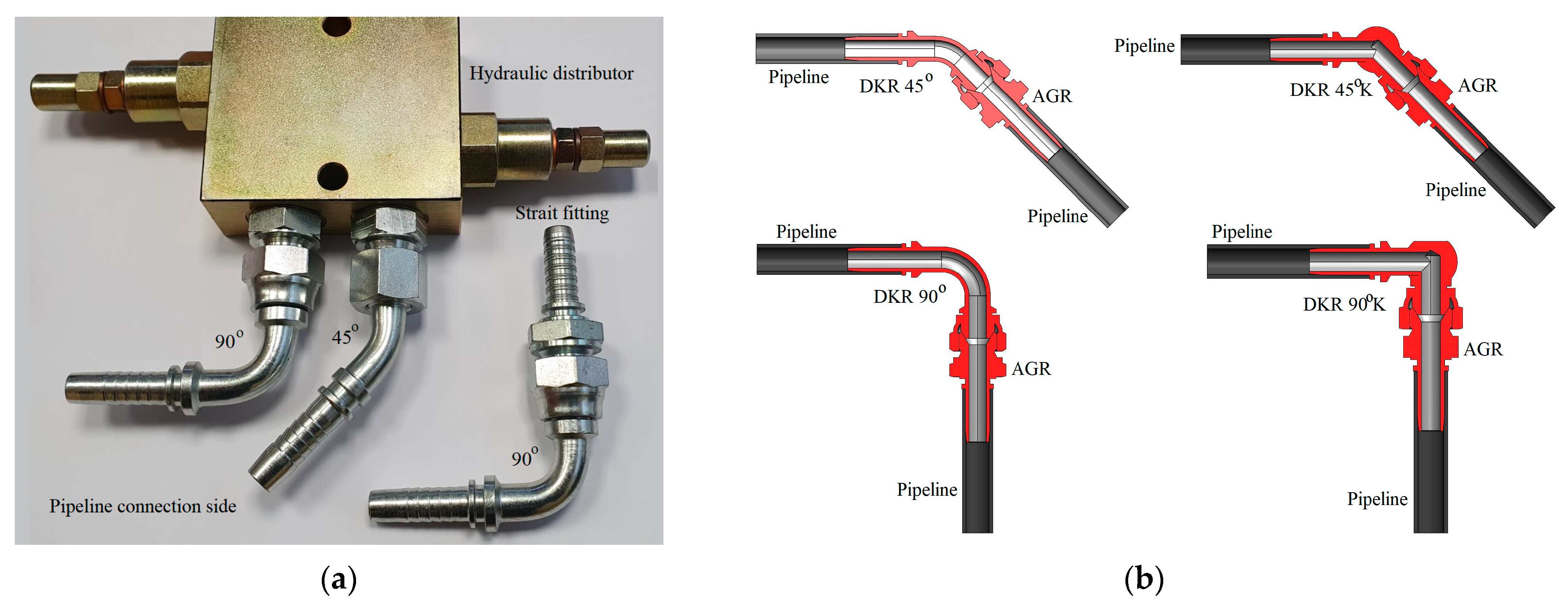
3. The Research Objects

The structures of pipeline connections in a hydraulic drive include the fittings (a nipple with a fixing nut or a connecting nipple) in connection with the hydraulic equipment (pumps, valves, throttles, cylinders, etc.), as shown in Figure 2a. According to [13], the most popular standards (BSP, British Standard Pipe cylindrical thread made according to the UK’s National Standard [34]) were selected for the current research. For simulation purposes, 3D models of the cross-section of angular fitting connections were created, as presented in Figure 2b. In addition, the following two types of angular fitting connections were compared: 45° and 90° DKR and DKR K.

The main issue is changes in the size and configuration of the cross-sectional area of the fluid flow in the fitting connections. The model of fluid flow in the connections of angular fittings in pipelines is shown in Figure 3.

In the current research, the 08 DASH (1/2” or 12.7 mm) conditional passage type of pipeline will be used because in [13] disclose that the pipeline standard of 08 DASH diameter of the conditional passage is one of the most frequently used diameters in hydraulic drives.

4. Fluid Flow Simulation inside Angular Fitting Connections

4.1. Numerical Formulation

The fluid flow inside angular fitting connections is simulated by solving 3D Navier–Stokes equations using ANSYS^® FLUENT^®. The fluid is assumed to be incompressible and represented by the conservation of momentum. The inlet and outlet flow boundary conditions are set as mass flow rate and total pressure with the convergence criterion of residual target as 10⁻⁵, according to the recommendation from [35,36]. The Reynolds-averaged Navier–Stokes (RANS) equations in 3D can be presented, according to [35,37], as the continuity equation:

$$\nabla \overrightarrow{u}=0.$$

(1)

The momentum equation:

$$\overrightarrow{u}\nabla u=-2\omega \times \overrightarrow{u}+{\omega }^2\overrightarrow{r}-\frac{1}{\rho }\nabla \overrightarrow{\tau },$$

(2)

where, $\overrightarrow{u}$ is the relative vector of fluid speed in a 3D environment; $\overrightarrow{r}$ is the radial location; ω is the angular speed of fluid near obstacles; $\overrightarrow{\tau }$ is the viscous stress. The viscous stress is a tensor quantity and is a combination of the viscous and turbulence viscosity terms:

$${\tau }_{ij}=2\nu \cdot s_{ij}-p\cdot u_i^{\prime }{u}_j^{\prime },$$

(3)

where, ν is the fluid viscosity; s_ij is the mean strain tensor; $p\cdot u_i^{\prime }{u}_j^{\prime }$ are the Reynolds stresses in 3D environment space.

4.2. Fluid Parameters and Numerical Model

Multiphase simulation involves a homogenous material, for example, standard mineral hydraulic oil (Hydraux HLP 46), that conforms to the German National Standard [38]. The properties of hydraulic oil used for numerical simulation can be found in [39]. Several boundary conditions are used for solving the incompressible RANS equations. Figure 4a shows an example of the applied boundary conditions with information about boundary layers for a wall boundary, an inlet boundary and outlet boundary conditions. The numerical simulation of fluid flow inside fitting connections was done by employing the ANSYS Workbench.

The numerical code was based on the FVM. The investigation area covered a 3D volume closed from all sides and divided into a mix of tetrahedral and pyramid elements. The mesh was refined near changes in the cross-sectional area and around a restrictive place, as necessary to obtain more accurate results. Close to the walls, boundary layers maximally affect velocity gradients in the normal direction to the wall. Five to seven inflation layers (IL) were created with an expansion factor of 1.1–1.5, depending on changes in the diameter and the shape of connections (see Figure 4b). The model was well validated in research [40] and was used for the current research. The main working parameters of the research bench for the validation model include: pressure in the hydraulic system is 2 MPa; the fluid flow rate is around 24 l/min; pipeline diameters are 1/2” (12.7 mm), which corresponds to pipeline used in current research.

The grid independence study was conducted through the creation of a different type of mesh for the angular fitting connection to determine the mesh quality affect on the CFD simulation results and to limit the maximum element size requirement (Figure 5a). The number of elements, primarily obtained results, simulation times and main characteristics of the mesh are shown in Figure 5b.

It is important to note that mesh resolution plays a pivotal role in the final CFD results. At G4, G5, and G6, the obtained results gave almost the same value. G4 and G6 give a nearly 3–4% difference in the estimated pressure drop, but the simulation time of the two meshes had a significant difference. Due to only a slight difference between G6 and G4 and lower computational costs, G4 was employed for the numerical analysis.

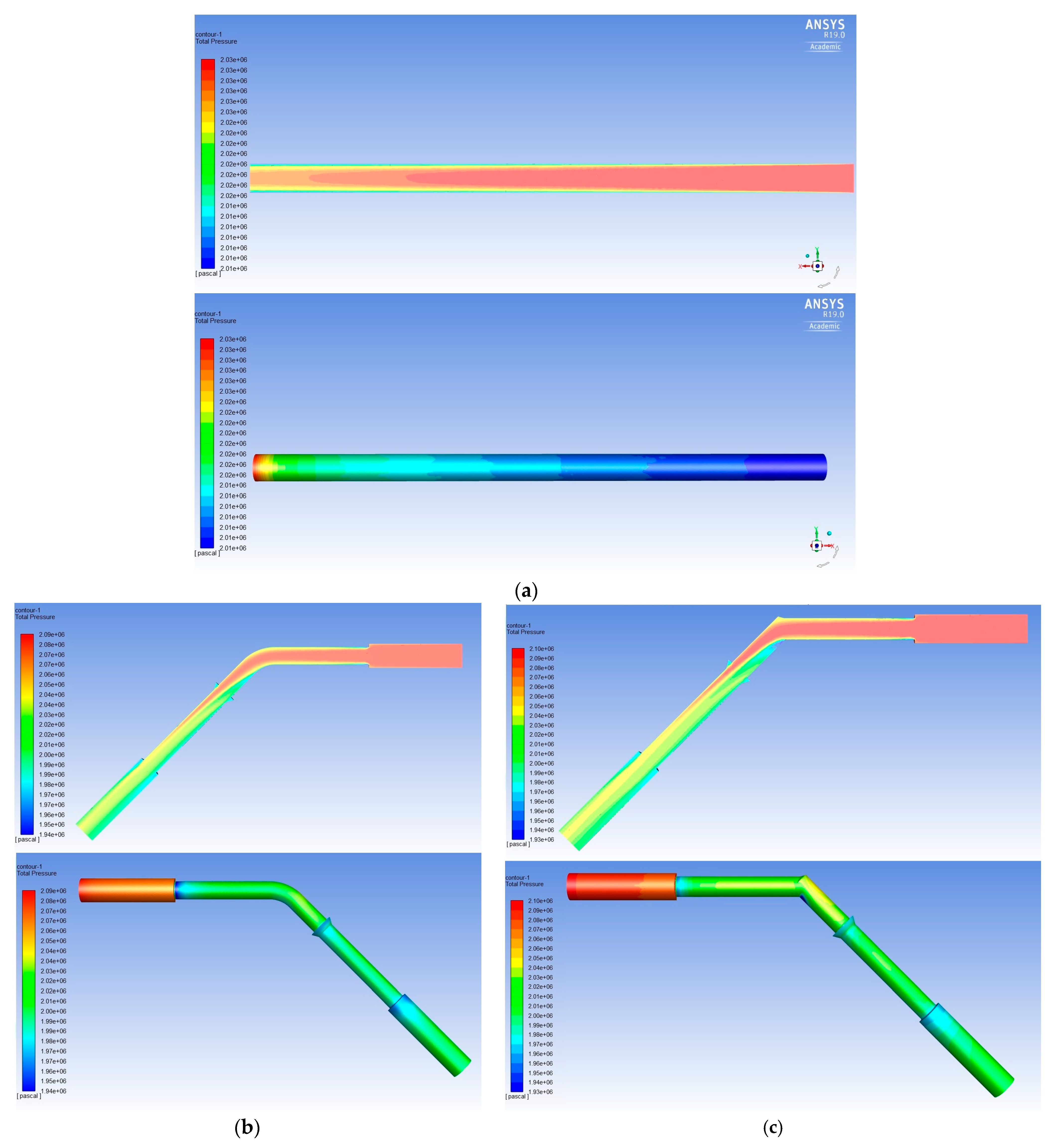
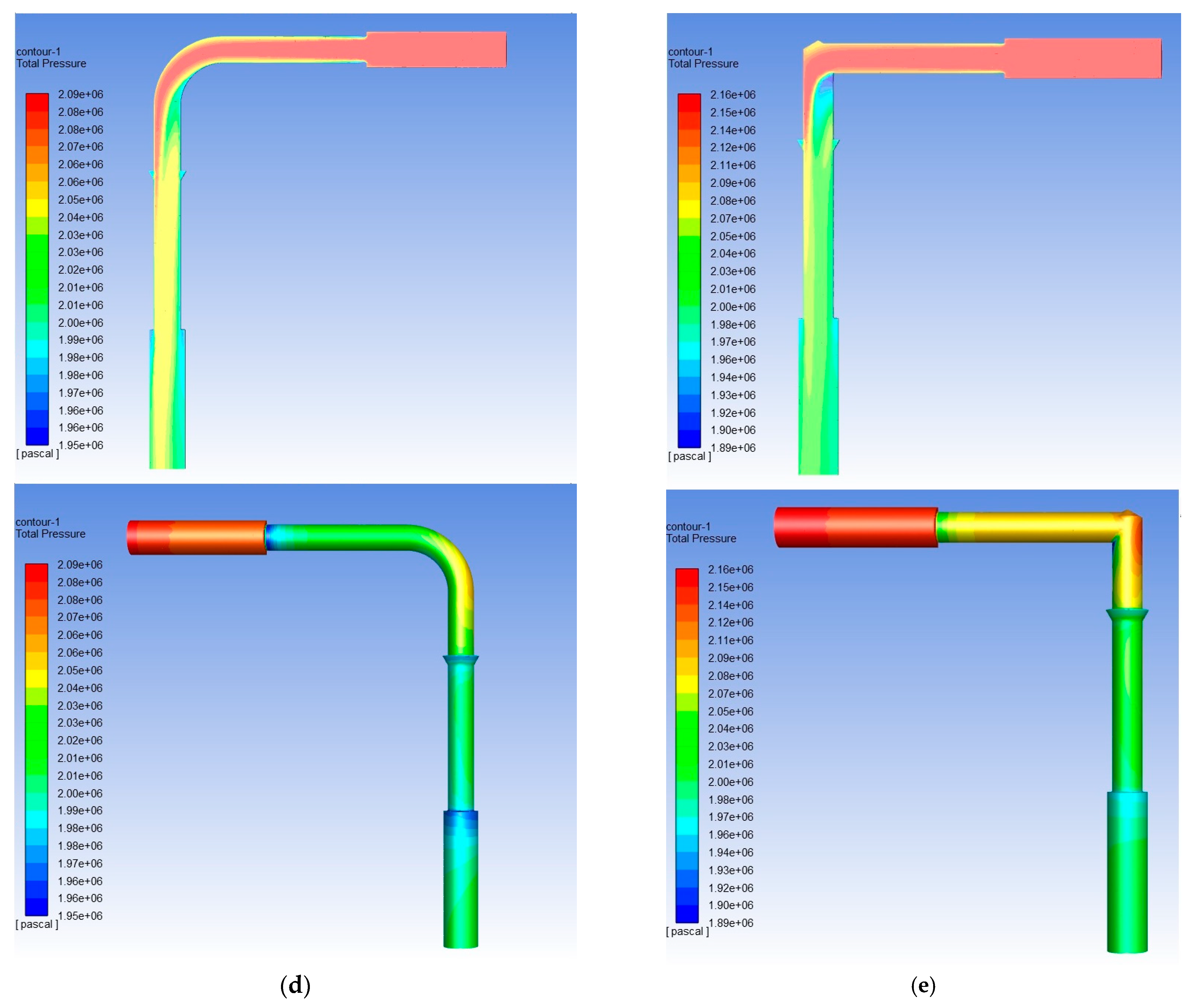
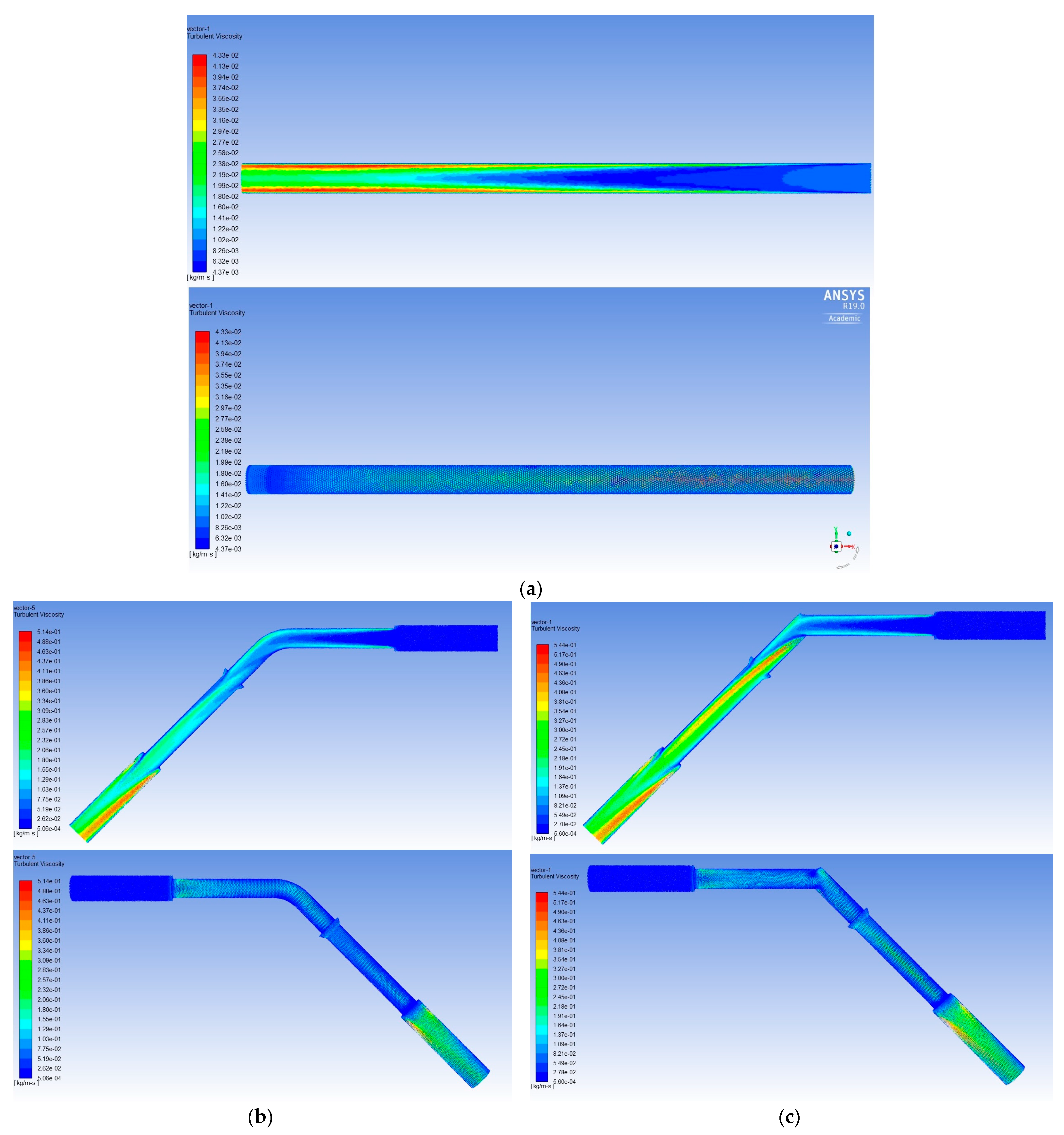
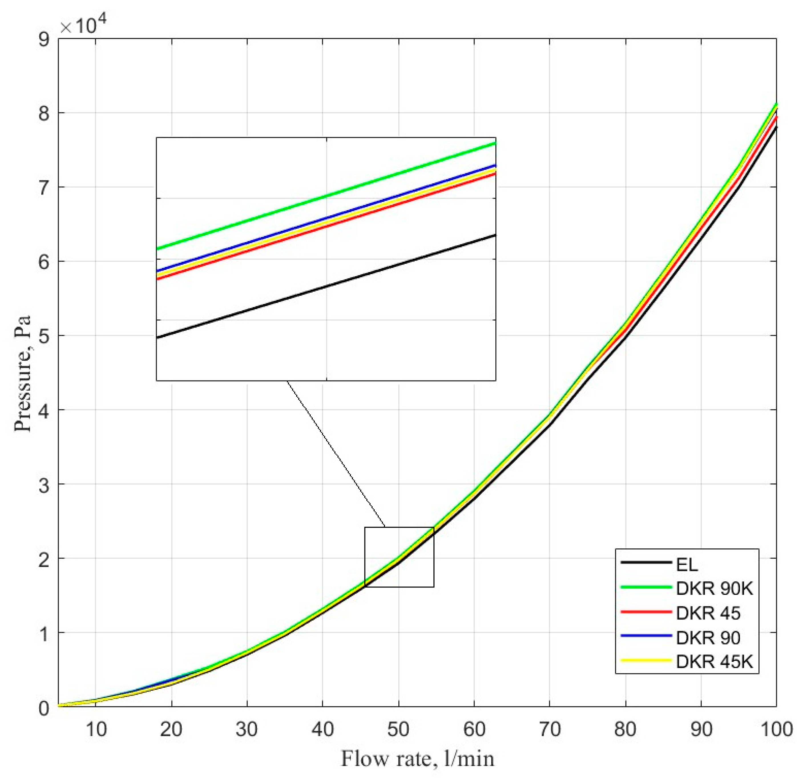
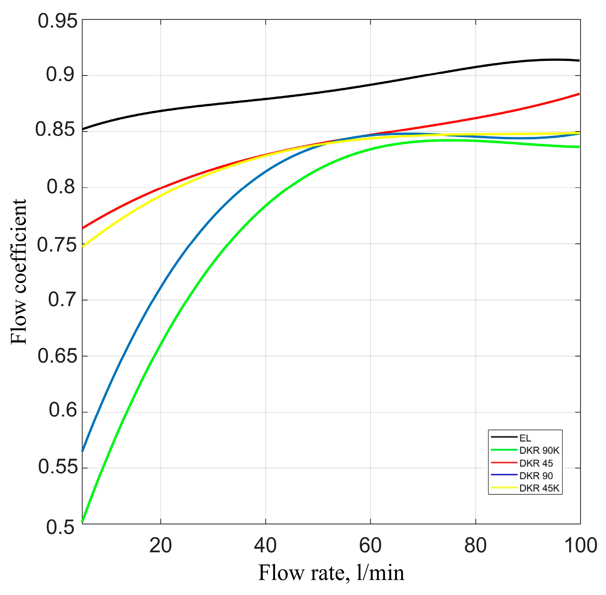
5. Results from the Numerical Simulation

The ANSYS Fluent simulation showed the gated fluid flow pressure drop at different angular fitting connections. For a better understanding and explanation of the obtained, the Reynolds number was calculated (see Figure 6). The total pressure profile of the fluid flow on angular fitting connections and the straight equivalent length are displayed in Figure 7. The additional results (turbulence processes) of the fluent simulation are provided in Figure 8. All displayed results were taken from ANSYS Fluent simulations where the inlet upload fluid velocity was 6.55 m/s (corresponded to the flow by 50 l/min, middle point of simulated flow rate range).

Pressure losses (power) at angular fitting connections were calculated for the range of researched flow rates and are presented in Figure 9. The flow coefficient is a relative measure of flow efficiency at an allowed fluid flow. The flow coefficient for fitting connections, also called the well-established orifice coefficient, can be found from the equation by [27,41]:

$$C_d=\frac{Q}{A\sqrt{\frac{1}{1-b^4}\sqrt{2\Delta p/\rho }}}$$

(4)

where, b = d/D b—diameter ratio; D—diameter of the pipeline, m; d—main diameter of fitting connection; Q—fluid flow rate; A—average cross-section area of pipeline before and after fitting connection; Δp—pressure drop; ρ—fluid density.

The flow coefficient describes the relationship between pressure drop across the fitting orifice and the corresponding fluid flow rate, and is a main characteristic when describing the fitting connection value, as shown in Figure 10. Energy losses at each angular fitting of hydraulic system are presented in

Table 1. Energy losses at angular fitting connections.

Flow Rate (l/min)	Pipeline (W)	DKR 90° (W)	DKR 90°K (W)	DKR 45° (W)	DKR 45°K (W)
5	1.52·10−3	5.22·10−3	5.91·10−3	3.81·10−3	4.24·10−3
10	1.22·10−2	3.84·10−2	4.08·10−2	2.42·10−2	2.98·10−2
15	4.21·10−2	7.76·10−2	9.26·10−2	5.77·10−2	6.29·10−2
20	0.125	0.343	0.378	0.241	0.283
25	0.238	0.452	0.498	0.322	0.391
30	0.353	0.597	0.677	0.366	0.413
35	0.558	0.825	0.995	0.632	0.708
40	0.465	1.023	1.237	0.897	0.934
45	1.212	1.598	1.778	1.223	1.409
50	1.367	1.887	2.078	1.573	1.669
55	1.768	2.451	2.642	2.284	2.327
60	2.312	3.207	3.482	2.798	2.988
65	2.671	3.846	3.998	3.562	3.629
70	3.523	4.745	4.955	4.532	4.707
75	4.624	5.923	6.073	5.182	5.496
80	5.735	7.121	7.411	6.247	6.724
85	7.989	8.998	9.209	8.273	8.629
90	8.557	10.875	11.342	9.057	9.522
95	10.142	13.517	13.782	11.347	11.808
100	11.177	16.261	16.663	13.438	14.113

(because it is difficult to show the difference in chart form). The standard relationship between pressure drops and flow rate inside a hydraulic drive was used to calculate the energy losses.

As clear from the Reynolds numbers provided in Figure 6, the turbulence of fluid flow through angular fitting connections started at a flow of ~30 l/min, and for equivalent length, at a rate of ~55 l/min. This confirms that the equivalent length method cannot be an accurate technique for calculating losses for angular fitting connections. The research objects were divided into three groups, for describing the obtained results:

Group Nr. 1—a straight pipeline with a length equivalent to the fitting connection;

Group Nr. 2—DKR 45° and DKR 45°K standard of angular fitting connections;

Group Nr. 3—DKR 90° and DKR 90°K standard of angular fitting connections.

The obtained results (flow coefficients) showed that group Nr. 1 had the most optimal flow characteristics (flow coefficient range: 0.851–0.903). Group Nr. 2 included the DKR 45° (flow coefficient range: 0.772–0.879), and the DKR 45°K (flow coefficient range: 0.749–0.85), which performed worse. Flow characteristics of group Nr. 3 embraced the DKR 90° (flow coefficient range: 0.572–0.9) and the DKR 90°K (flow coefficient range: 0.512–0.841), which performed the least effectively due to significant changes in the cross-sectional area and shapes of the angular fitting connection. Group Nr.1 presented an ideal section of the pipeline with no changes in the cross-sectional area, whereas groups Nr. 2 and Nr. 3 pointed out changes in cross-sectional areas and shape of fluid flow.

The difference between changes in the cross-sectional areas of standard angular fittings and their K-type had a significant impact on flow characteristics. The difference between flow coefficients for standard angular fittings and their K-type was around 10% for group Nr. 2 and ~15% for group Nr. 3 at the beginning of the chart. Also, a significant difference in flow characteristics at different flow processes inside angular fitting connections was observed. Unlike groups Nr. 2 and Nr. 3, other groups had no significant differences in the processes of the turbulent flow (according to the uploaded boundary conditions). However, in terms of the turbulence of flow processes, groups Nr. 2 and Nr. 3 had similar flow characteristics. Research on power losses in group Nr. 1 demonstrated insignificant power losses (1.52·10⁻³–11.177 W) compared to group Nr. 2 which included the DKR 45° (range, 3.81·10⁻³–13.438 W) and DKR 45°K (range, 4.24·10⁻³–14.113 W) standards. Higher power losses were observed in group Nr. 3, which had the DKR 90° (range, 5.22·10⁻³–16.261 W) and DKR 90°K (range, 5.91·10⁻³–16.663 W) standards.

The results of the modelling showed that the equivalent length method cannot be accepted as an accurate technique for calculating energy losses, flow coefficient, etc. in the angular fitting connections. The research disclosed that standard methods for calculating hydraulic fittings were not accurate and that each type of angular fitting connection requires additional investigation.

6. Conclusions

This research analysed the influence of hydrodynamic processes on the fluid flow characteristics following installation of angular fitting connections in pipeline systems. The analysis was done through numerical simulations using the RANS equations in 3D. The dynamics of fluid flow in the hydraulic system were investigated by taking into account the main parameters of a flow rate up to 100 l/min. To simulate fluid flow, six different mesh independence studies were performed. As a result, pressure drop, turbulence model, energy losses and flow coefficients for two types of 45° and 90° angular fitting connections were obtained.

It was found that the turbulence of fluid flow through angular fitting connections started at a flow of ~30 l/min, and for equivalent length, at a rate of ~55 l/min. This confirms that equivalent length method cannot be an accurate technique for calculating losses for angular fitting connections. Differences between changes in the cross-sectional areas of standard angular fittings and their K-type had a significant impact on flow characteristics. There was a difference between flow coefficients for standard angular fittings and their K-type, which was around 10% for group Nr. 2 and ~15% for group Nr. 3 at the beginning of the chart. Research on power losses in group Nr. 1 demonstrated insignificant power losses (1.52·10⁻³–11.177 W) compared to group Nr. 2 which included the DKR 45° (range, 3.81·10⁻³–13.438 W) and DKR 45°K (range, 4.24·10⁻³–14.113 W) standards. Higher power losses were observed in group Nr. 3, which had the DKR 90° (range, 5.22·10⁻³–16.261 W) and DKR 90°K (range, 5.91·10⁻³–16.663 W) standards.

The performed research showed that using the equivalent length method is incorrect for investigation into angular fitting connections, and that each type of angular fitting connection requires additional investigations. Thus, a worthwhile investigation for future research would be into the flow characteristics of a hydraulic connection on backflow, because fluid moves in both directions of the connections.

References

1. Karpenko, M.; Bogdevičius, M. Review of energy-saving technologies in modern hydraulic drives. Sci. Future Lith. Moksl. Liet. Ateitis 2017, 9, 553–558. [Google Scholar] [CrossRef] [Green Version]
2. Bogdevičius, P.; Prentkovskis, O.; Bogdevičius, M. Transmission with cardan joint parametre influence to centrifugal pump characteristics. Moksl. Liet. Ateitis/Sci. Future Lith. 2017, 9, 559–564. [Google Scholar] [CrossRef] [Green Version]
3. Parvaresh, A.; Mardani, M. Model predictive control of a hydraulic actuator in torque applying system of a mechanically closed-loop test rig for the helicopter gearbox. Aviation 2019, 23, 143–153. [Google Scholar] [CrossRef]
4. Di Gialleonardo, E.; Santelia, M.; Bruni, S.; Zolotas, A. A simple active carbody roll scheme for hydraulically actuated railway vehicles using internal model control. ISA Trans. 2021, 120, 55–69. [Google Scholar] [CrossRef]
5. Wei, Q.; Huailiang, Z.; Wenqian, S.; Wei, L. Stress response of the hydraulic composite pipe subjected to random vibration. Compos. Struct. 2021, 255, 112958. [Google Scholar] [CrossRef]
6. Lubecki, M.; Stosiak, M.; Bocian, M.; Urbanowicz, K. Analysis of selected dynamic properties of the composite hydraulic microhose. Eng. Fail. Anal. 2021, 125, 105431. [Google Scholar] [CrossRef]
7. Nishimura, S.; Matsunaga, T. Analysis of response lag in hydraulic power steering system. JSAE Rev. 2000, 21, 41–46. [Google Scholar] [CrossRef]
8. European Commission. Communication from the Commission to the European Parliament, the Council, the European Economic and Social Committee and the Committee of the Regions. Brussels, Belgium, 2011. Available online: https://eur-lex.europa.eu/LexUriServ/LexUriServ.do?uri=COM:2011:0885:FIN:EN:PDF (accessed on 20 January 2023).
9. Yan, X.; Chen, B.; Zhang, D.; Wu, C.; Luo, W. An energy-saving method to reduce the installed power of hydraulic press machines. J. Clean. Prod. 2019, 233, 538–545. [Google Scholar] [CrossRef]
10. Moraesa, M.; Muiños, D. Experimental quantification of the head loss coefficient K for fittings and semi-industrial pipe cross section solid concentration profile in pneumatic conveying of polypropylene pellets in dilute phase. Int. J. Sci. Technol. Powder Technol. 2017, 310, 250–263. [Google Scholar] [CrossRef]
11. Zhao, K.; Liu, Z.; Yu, S.; Li, X.; Huang, H.; Li, B. Analytical energy dissipation in large and medium-sized hydraulic press. J. Clean. Prod. 2015, 103, 908–915. [Google Scholar] [CrossRef]
12. Kong, X.; Majumdar, H.; Zang, F.; Jiang, S.; Wu, Q.; Zhang, W. A multi-switching mode intelligent hybrid control of electro-hydraulic proportional systems. Proc. Inst. Mech. Eng. Part C J. Mech. Eng. Sci. 2019, 233, 120–131. [Google Scholar] [CrossRef]
13. Karpenko, M.; Bogdevičius, M. Investigation into the hydrodynamic pro-cesses of fitting connections for determining pressure losses of transport hydraulic drive. Transport 2020, 35, 108–120. [Google Scholar] [CrossRef] [Green Version]
14. EN 853 2SN:2015; Rubber hoses and hose assemblies. Wire braid reinforced hydraulic type. European Commission on Standardisation: Geneva, Switzerland, 2015; 17p.
15. ISO 8331:2016; Rubber and plastics hoses and hose assemblies—Guidelines for selection, storage, use and maintenance. International Standard Organisation: Geneva, Switzerland, 2016; 13p.
16. Parker Hannifin Ltd. Hydraulic Hoses, Fittings and Equipment. Technical Handbook, 2019; 84. Bulletin BUL/C4400-A/UK. Available online: https://www.parker.com/Literature/Polymer%20Hose%20Division%20Europe/Sales%20and%20Marketing%20Bulletins/4400_Rubber%20Hydraulic/Technical%20Handbook-UK.pdf (accessed on 21 January 2023).
17. Yokohama Rubber Co. Hose and Fittings, the Products of YOKOHAMA. Catalog Number 905-1, 2014; 106. Available online: https://www.y-yokohama.com/global/mb/pdf/resource/hose-and-fittings.pdf (accessed on 21 January 2023).
18. Speedflow. AN Hose and Fitting Guide. 2014. Available online: https://anfittingguide.com/wp-content/uploads/2014/01/AN-hose-and-fitting-guide-v21.pdf (accessed on 23 January 2023).
19. Gates Corporation. A Guide to Preventive Maintenance & Safety for Hydraulic Hose & Couplings. Tomkins Company. 2009. Available online: http://www.marshall-equipement.com/Library/SafeHydraulics.pdf (accessed on 22 January 2023).
20. Eaton. Eaton Hydraulic Hose and Tubing. Safety Guide. 2020, p. 12. Available online: https://www.eaton.com/ecm/groups/public/@pub/@eaton/@hyd/documents/content/pct_4085913.pdf (accessed on 18 January 2023).
21. Błażejewski, R.; Matz, R.; Nawrot, T.; Rudzik, D. Reliability and optimal replacement interval of flexible hose assemblies in drinking water installations. Eng. Fail. Anal. 2020, 109, 104327. [Google Scholar] [CrossRef]
22. Chuang, G.; Ferng, Y. Investigating effects of injection angles and velocity ratios on thermal-hydraulic behavior and thermal striping in a T-junction. Int. J. Therm. Sci. 2018, 126, 74–81. [Google Scholar] [CrossRef]
23. Crane Co. Flow of Fluids through Valves, Fittings and Pipe. Metric Edition—Si Units; Technical Paper; Crane Co.: New York, NY, USA, 1982; 133p. [Google Scholar]
24. Bojko, M.; Kozubkova, M. Investigation of hydraulic fitting losses. In Proceedings of the XXI International Scientific Conference—The Application of Experimental and Numerical Methods in Fluid Mechanics and Energy, Cracow, Poland, 25–27 November 2018; Volume 168, pp. 1–10. [Google Scholar] [CrossRef] [Green Version]
25. Valdes, J.; Rodrigues, J.; Saumell, J.; Putz, T. A methodology for the parametric modelling of the flow coefficients and flow rate in hydraulic valves. Energy Convers. Manag. 2017, 88, 598–611. [Google Scholar] [CrossRef]
26. Crane Valve Co. Flow of Fluids Through Valves, Fittings, and Pipe; Technical Paper no. 410; Crane Co.: New York, NY, USA, 1998; 132p. [Google Scholar]
27. Hooper, W. The two-K method predicts head losses in pipe fittings. Chem. Eng. 1981, 88, 96–100. [Google Scholar]
28. Stosiak, M.; Skačkauskas, P.; Towarnicki, K.; Deptuła, A.; Deptuła, A.M.; Prażnowski, K.; Grzywacz, Ż.; Karpenko, M.; Urbanowicz, K.; Łapka, M. Analysis of the Impact of Vibrations on a Micro-Hydraulic Valve Using a Modified Induction Algorithm. Machines 2023, 11, 184. [Google Scholar] [CrossRef]
29. Catellani, C.; Cazzoli, G.; Falfari, S.; Forte, C.; Bianchi, G. Large eddy simulation of a steady flow test bench using OpenFOAM. Energy Procedia 2016, 101, 622–629. [Google Scholar] [CrossRef]
30. Li, D.; Fu, X.; Zuo, Z.; Wang, H.; Li, Z.; Liu, S.; Wei, X. Investigation methods for analysis of transient phenomena concerning design and operation of hydraulic-machine systems—A review. Renew. Sustain. Energy Rev. 2019, 101, 26–46. [Google Scholar] [CrossRef]
31. Gai, Y.; Kimiabeigi, M.; Chong, Y.; Widmer, J.; Deng, X.; Popescu, M. Cooling of automotive traction motors: Schemes, examples and computation methods—A review. IEEE Trans. Ind. Electron. 2019, 66, 1681–1692. [Google Scholar] [CrossRef] [Green Version]
32. Akin, A.; Kahveci, H. Effect of turbulence modeling for the prediction of flow and heat transfer in rotorcraft avionics bay. Aerosp. Sci. Technol. 2019, 95, 105453. [Google Scholar] [CrossRef]
33. Liu, H.; Zhang, X.; Quan, L.; Zhang, H. Research on energy consumption of injection molding machine driven by five different types of electro-hydraulic power units. J. Clean. Prod. 2020, 242, 118355. [Google Scholar] [CrossRef]
34. BS EN 10226-2:2005; Pipe threads where pressure-tight joints are not made on the threads—Part 1: Dimensions, tolerances and designation. British National Standard: London, UK; European Committee for Standardization: Brussels, Belgium, 2005; 16p.
35. Kim, B.; Siddique, M.; Samad, A.; Hu, G.; Lee, D. Optimization of centrifugal pump impeller for pumping viscous Fluids Using Direct Design Optimization Technique. Machines 2022, 10, 774. [Google Scholar] [CrossRef]
36. Urbanowicz, K.; Bergant, A.; Stosiak, M.; Deptuła, A.; Karpenko, M. Navier-Stokes Solutions for Accelerating Pipe Flow—A Review of Analytical Models. Energies 2023, 16, 1407. [Google Scholar] [CrossRef]
37. Santos, F.; Brito, A.; de Castro, A.; Almeida, M.; da Cunha Lima, A.; Zebende, G.; da Cunha Lima, I. Detection of the persistency of the blockages symmetry on the multi-scale cross-correlations of the velocity fields in internal turbulent flows in pipelines. Phys. A Stat. Mech. Appl. 2018, 509, 294–301. [Google Scholar] [CrossRef]
38. DIN 51524-2; Pressure Fluids—Hydraulic oils—Part 2: HLP Hydraulic oils, Minimum Requirements. German National Standard. Standard Specification; DIN Deutsches Institut für Normung e. V.: Berlin, Germany, 2017; 11p.
39. Karpenko, M.; Prentkovskis, O.; Šukevičius, Š. Research on high-pressure hose with repairing fitting and influence on energy parameter of the hydraulic drive. Eksploat. Niezawodn. Maint. Reliab. 2022, 24, 25–32. [Google Scholar] [CrossRef]
40. Karpenko, M. Investigation of Energy Efficiency of Mobile Machinery Hydraulic Drives. Ph.D. Thesis, Vilnius Gediminas Technical University, Vilnius, Lithuania, 2021; 164p. [Google Scholar] [CrossRef]
41. ISO 5167-1:2022; Measurement of Fluid Flow by Means of Orifice Plates, Nozzles, and Venturi Tubes Inserted in Circular Cross Section Conduits Running Full. European Commission on Standardisation: Geneva, Switzerland, 2022; p. 42.
Figure 1. Composition of a typical hydraulic drive system: (a) part of a machine hydraulic drive system; (b) recommendation according to high-pressure hoses installation.
Machines 11 00355 g001
Figure 2. Fittings used in the research: (a) Connection of angular fittings in a hydraulic system; (b) Cross-section of angular fitting connections in 3D pipelines models.
Machines 11 00355 g002
Figure 3. Model of fluid flow in the connections of angular fittings in pipelines.
Machines 11 00355 g003
Figure 4. Views of the numerical simulation model for angular fitting connections (1/2): (a) boundary conditions of the fluid flow for ANSYS fluent simulation; (b) example mesh of the numerical model.
Machines 11 00355 g004
Figure 5. Views of the numerical simulation model for angular fitting connections (2/2): (a) mesh resolution; (b) summarised results from grid independence study.
Machines 11 00355 g005aMachines 11 00355 g005b
Figure 6. The Reynolds number of flow rate for angular fitting connections.
Machines 11 00355 g006
Figure 7. View of the total fluid flow pressure across angular fitting connections (top—symmetry side; bottom—wall side): (a) equivalent length method; (b) DKR 45° connection; (c) DKR 45°K connection; (d) DKR 90° connection; (e) DKR 90°K connection.
Machines 11 00355 g007aMachines 11 00355 g007b
Figure 8. View of the fluid flow turbulence processes across angular fitting connections (top—symmetry side; bottom—wall side): (a) equivalent length method; (b) DKR 45° connection; (c) DKR 45°K connection; (d) DKR 90° connection; (e) DKR 90°K connection.
Machines 11 00355 g008aMachines 11 00355 g008b
Figure 9. Fluid pressure losses at the angular fitting connections.
Machines 11 00355 g009
Figure 10. Flow coefficient of angular fitting connections.
Machines 11 00355 g010