
YOLO-v1 to YOLO-v8, the Rise of YOLO and Its Complementary Nature toward Digital Manufacturing and Industrial Defect Detection

Department of Computer Science, School of Computing and Engineering, University of Huddersfield, Queensgate, Huddersfield HD1 3DH, UK
Machines 2023, 11(7), 677; https://doi.org/10.3390/machines11070677
Submission received: 30 May 2023
/
Revised: 15 June 2023
/
Accepted: 21 June 2023
/
Published: 23 June 2023
(This article belongs to the Special Issue State-of-the-Art in Digital Manufacturing Systems)
Abstract
:Since its inception in 2015, the YOLO (You Only Look Once) variant of object detectors has rapidly grown, with the latest release of YOLO-v8 in January 2023. YOLO variants are underpinned by the principle of real-time and high-classification performance, based on limited but efficient computational parameters. This principle has been found within the DNA of all YOLO variants with increasing intensity, as the variants evolve addressing the requirements of automated quality inspection within the industrial surface defect detection domain, such as the need for fast detection, high accuracy, and deployment onto constrained edge devices. This paper is the first to provide an in-depth review of the YOLO evolution from the original YOLO to the recent release (YOLO-v8) from the perspective of industrial manufacturing. The review explores the key architectural advancements proposed at each iteration, followed by examples of industrial deployment for surface defect detection endorsing its compatibility with industrial requirements.
1. Introduction
Humans via the visual cortex, a primary cortical region of the brain responsible for processing visual information [1], are able to observe, recognize [2], and differentiate between objects instantaneously [3]. Studying the inner workings of the visual cortex and the brain in general has paved the way for artificial neural networks (ANNs) [4] along with a myriad of computational architectures residing under the deep learning umbrella. In the last decade, owing to rapid and revolutionary advancements in the field of deep learning [5], researchers have exerted their efforts on providing efficient simulation of the human visual system to computers, i.e., enabling computers to detect objects of interest within static images and video [6], a field known as computer vision (CV) [7]. CV is a prevalent research area for deep learning researchers and practitioners in the present decade. It is composed of subfields consisting of image classification [8], object detection [9], and object segmentation [10]. All three fields share a common architectural theme, namely, manipulation of convolutional neural networks (CNNs) [11]. CNNs are accepted as the de facto when dealing with image data. In comparison with conventional image processing and artificial defection methods, CNNs utilize multiple convolutional layers coupled with aggregation, i.e., pooling structures aiming to unearth deep semantic features hidden away within the pixels of the image [12].
Artificial intelligence (AI) has found opportunities in industries across the spectrum from renewable energy [13,14] and security to healthcare [15] and the education sector. However, one industry that is poised for significant automation through CV is the manufacturing industry. Quality inspection (QI) is an integral part of any manufacturing domain providing integrity and confidence to the clients on the quality of the manufactured products [16]. Manufacturing has wide scope for automation; however, when dealing with surface inspection [17], defects can take sophisticated forms [18], making human-based quality inspection a cumbersome task with manifold inefficiencies linked to human bias, fatigue, cost, and downtime [19]. These inefficiencies provide an opportunity for CV-based solutions to present automated quality inspection that can be integrated within existing surface defect inspection processes, increasing efficiency whilst overcoming bottlenecks presented via conventional inspection methodologies [20].
However, for success, CV-based architectures must conform to a stringent set of deployment requirements that can vary from one manufacturing sector to another [21]. In the majority of applications, the focus is not only on the determination of the defect, but also on multiple defects along with the locality details of each [22]. Therefore, object detection is preferred over image classification since the latter only focuses on determination of object within the image without providing any locality information. Architectures within the object detection domain can be classified into single-stage or two-stage detectors [23]. Two-stage detectors split the detection process into two stages: Feature extraction/proposal followed by regression and classification for acquiring the output [24]. Although this can provide high accuracy, it comes with a high computational demand making it inefficient for real-time deployment onto constrained edge devices. Single-stage detectors, on the other hand, merge the two processes into one, enabling the classification and regression via a single pass, significantly reduce the computational demand, and provide a more compelling case for production-based deployment [25]. Although many single-stage detectors have been introduced, such as single shot detector (SSD) [26], deconvolutional single shot detector (D-SSD) [27], and RetinaNet [28], the YOLO (You Only Look Once) [29] family of architectures seems to be gaining high traction due to its high compatibility with industrial requirements, such as accuracy, lightweight, and edge-friendly deployment conditions. The last half-a-decade has been dominated by the introduction of YOLO variants, with the most recent variant introduced in 2022 as YOLO-v8.
To the best of our knowledge, there is no cohesive review of the advancing YOLO variants, benchmarking technical advancements, and their implications on industrial deployment. This paper reviews the YOLO variants released to the present date, focusing on presenting the key technical contributions of each YOLO iteration and its impact on key industrial metrics required for deployment, such as accuracy, speed, and computational efficacy. As a result, the aim is to provide researchers and practitioners with a better understanding of the inner workings of each variant, enabling them to select the most relevant architecture based on their industrial requirements. Additionally, literature on the deployment of YOLO architectures for various industrial surface defect detection applications is presented.
The subsequent structure of the review is as follows. The first section provides an introduction to single- and two-stage detectors and the anatomy for single-stage object detectors. Next, the evolution of YOLO variants is presented, detailing the key contributions from YOLO-v1 to YOLO-v8, followed by a review of the literature focused on YOLO-based implementation of industrial surface defect detection. Finally, the discussion section focuses on summarizing the reviewed literature, followed by extracted conclusions, future directions, and challenges are presented.
Object Detection
CNNs can be categorized as convolution-based feed forward neural networks for classification purposes [30]. The input layer is followed by multiple convolutional layers to acquire an increased set of smaller-scale feature maps. These feature maps post further manipulation are transformed into one-dimensional feature vectors before being used as input to the fully connected layer(s). The process of feature extraction and feature map manipulation is vital to the overall accuracy of the network; therefore, this can involve the stacking of multiple convolutional and pooling layers for richer feature maps. Popular architectures for feature extraction include AlexNet [31], VGGNet [32], GoogleNet [33], and ResNet [34]. AlexNet is proposed in 2012 and consists of five convolutional, three pooling, and three fully connected layers primarily utilized for image classification tasks. VGGNet focused on performance enhancement by increasing the internal depth of the architecture, introducing several variants with increased layers, VGG-16/19. GoogleNet introduced the cascading concept by cascading multiple ‘inception’ modules, whilst ResNet introduced the concept of skip-connections for preserving information and making it available from the earlier to the later layers of the architecture.
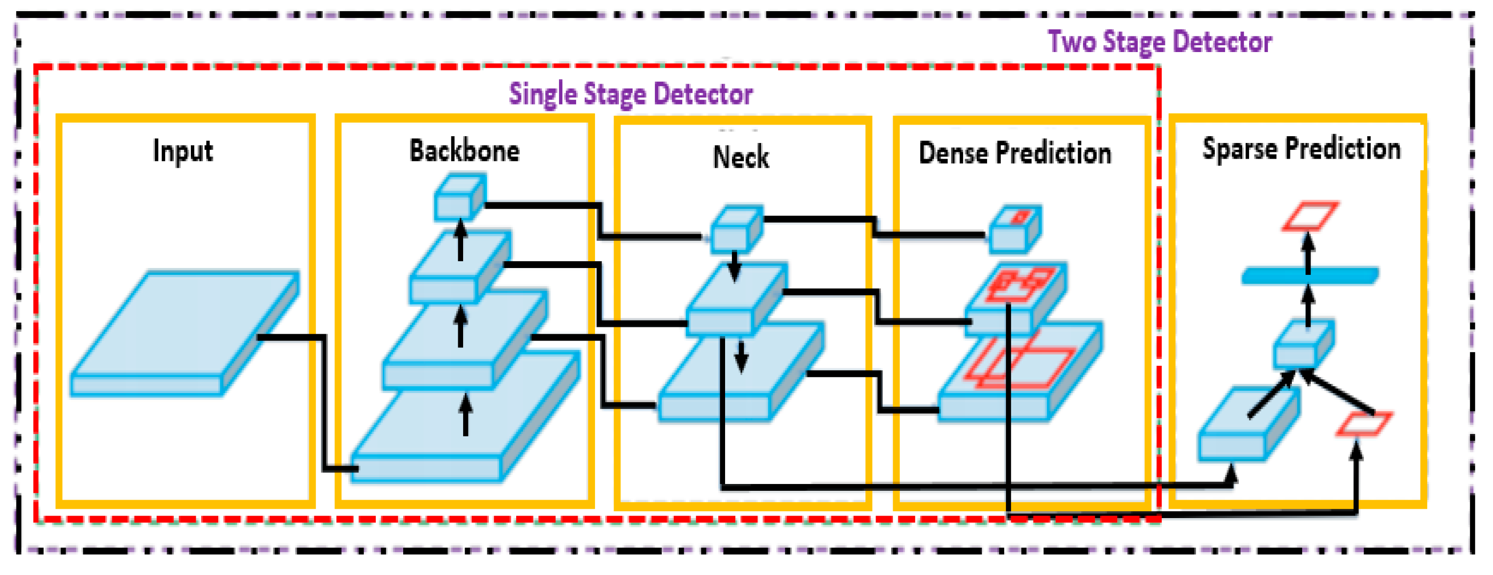
The motive for an object detector is to infer whether the object(s) of interest are residing in the image or present the frame of a video. If the object(s) of interest are present, the detector returns the respective class and locality, i.e., location dimensions of the object(s). Object detection can be further divided into two sub-categories: Two-stage methods and one-stage methods as shown in Figure 1. The former initiates the first stage with the selection of numerous proposals, then in the second stage, performs prediction on the proposed regions. Examples of two-stage detectors include the famous R-CNN [35] variants, such as Fast R-CNN [36] and Faster R-CNN [37], boasting high accuracies but low computational efficiency. The latter transforms the task into a regression problem, eliminating the need for an initial stage dedicated to selecting candidate regions; therefore, the candidate selection and prediction is achieved in a single pass. As a result, architectures falling into this category are computationally less demanding, generating higher FPS and detection speed, but in general the accuracy tends to be inferior with respect to two-stage detectors.
2. Original YOLO Algorithm
YOLO was introduced to the computer vision community via a paper release in 2015 by Joseph Redmon et al. [29] titled ‘You Only Look Once: Unified, Real-Time Object Detection’. The paper reframed object detection, presenting it essentially as a single pass regression problem, initiating with image pixels and moving to bounding box and class probabilities. The proposed approach based on the ‘unified’ concept enabled the simultaneous prediction of multiple bounding boxes and class probabilities, improving both speed and accuracy.
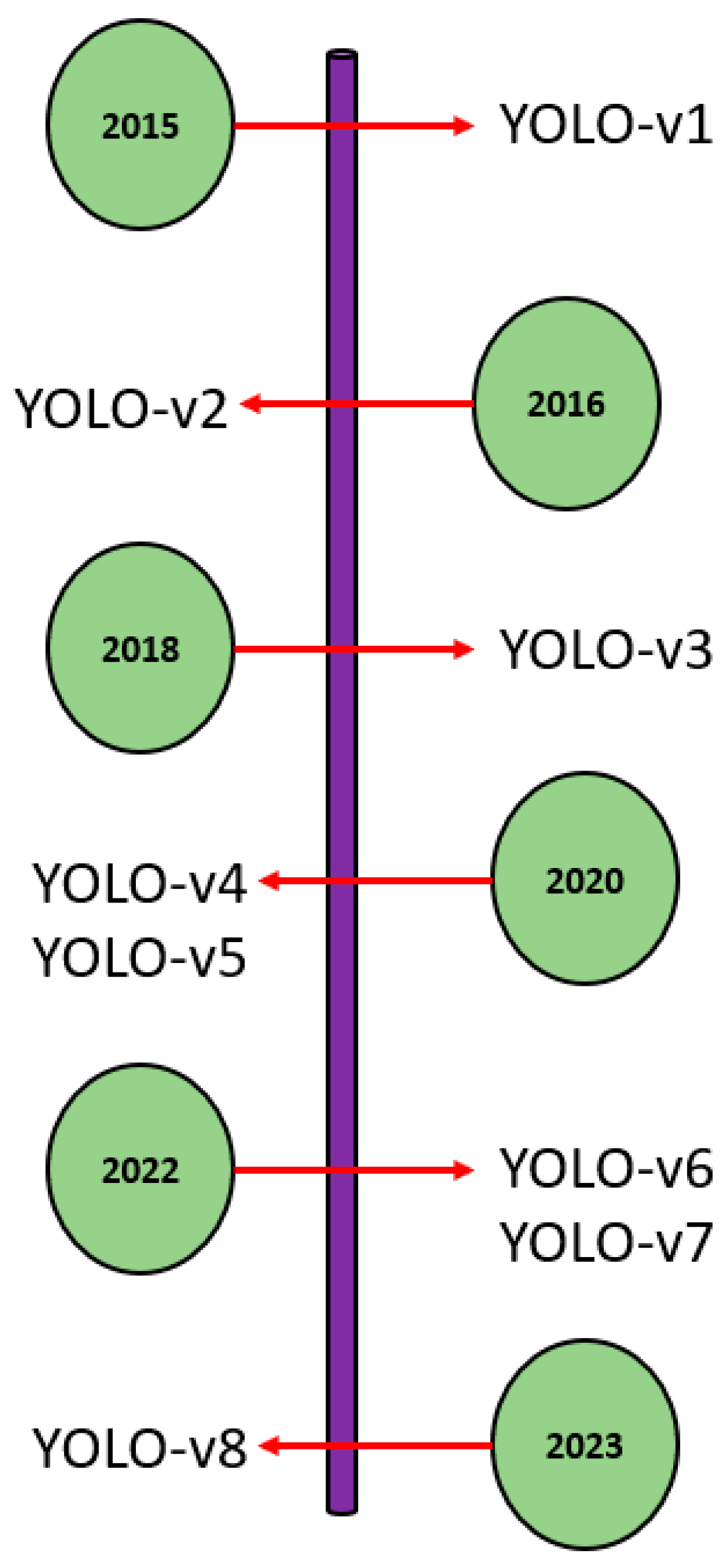
Since its inception in 2016 until the present year (2023), the YOLO family has continued to evolve at a rapid pace. Although the initial author (Joseph Redmon) halted further work within the computer vision domain at YOLO-v3 [38], the effectiveness and potential of the core ‘unified’ concept have been further developed by several authors, with the latest addition to the YOLO family coming in the form of YOLO-v8. Figure 2 presents the YOLO evolution timeline.
2.1. Original YOLO
The core principle proposed by YOLO-v1 was the imposing of a grid cell with dimensions of s×s onto the image. In the case of the center of the object of interest falling into one of the grid cells, that particular grid cell would be responsible for the detection of that object. This permitted other cells to disregard that object in the case of multiple appearances.
For implementation of object detection, each grid cell would predict B bounding boxes along with the dimensions and confidence scores. The confidence score was indicative of the absence or presence of an object within the bounding box. Therefore, the confidence score can be expressed as Equation (1):
where signified the probability of the object being present, with a range of 0–1 with 0 indicating that the object is not present and represented the intersection-over-union with the predicted bounding box with respect to the ground truth bounding box.
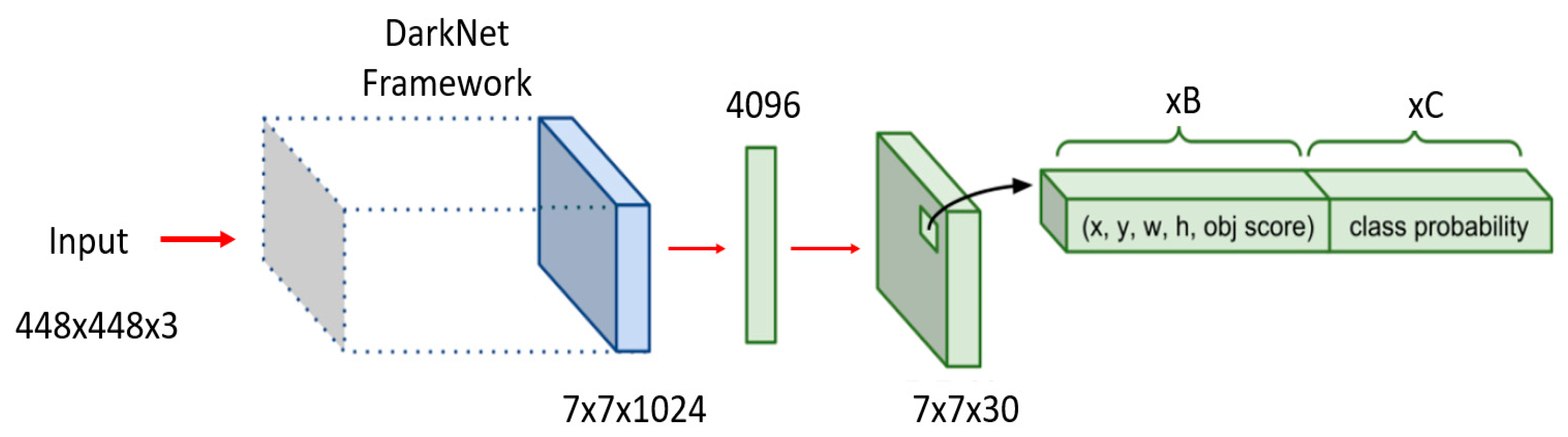
Each bounding box consisted of five components (x, y, w, h, and the confidence score) with the first four components corresponding to center coordinates (x, y, width, and height) of the respective bounding box as shown in Figure 3.
As alluded to earlier, the input image is split into s × s grid cells (default = 7 × 7), with each cell predicting B bounding boxes, each containing five parameters and sharing prediction probabilities of classes (C). Therefore, the parameter output would take the following form, expressed in (2):
Considering the example of YOLO network with each cell bounding box prediction set to 2 and evaluating the benchmark COCO dataset consisting of 80 classes, the parameter output would be given as expressed in (3):
The fundamental motive of YOLO and object detection in general is the object detection and localization via bounding boxes. Therefore, two sets of bounding box vectors are required, i.e., vector y is the representative of ground truth and vector is the predicted vector. To address multiple bounding boxes containing no object or the same object, YOLO opts for non-maximum suppression (NMS). By defining a threshold value for NMS, all overlapping predicted bounding boxes with an IoU lower than the defined NMS value are eliminated.
The original YOLO based on the Darknet framework consisted of two sub-variants. The first architecture comprised of 24 convolutional layers with the final layer providing a connection into the first of the two fully connected layers. Whereas the ‘Fast YOLO’ variant consisted of only nine convolutional layers hosting fewer filters each. Inspired by the inception module in GoogleNet, a sequence of convolutional layers was implemented for reducing the resultant feature space from the preceding layers. The preliminary architecture for YOLO-v1 is presented in Figure 3.
To address the issue of multiple bounding boxes for the same object or with a confidence score of zero, i.e., no object, the authors decided to greatly penalize predictions from bounding boxes containing objects () and the lowest penalization for prediction containing no object (). The authors calculated the loss function by taking the sum of all bounding box parameters (x, y, width, height, confidence score, and class probability). As a result, the first part of the equation computes the loss of the bounding box prediction with respect to the ground truth bounding box based on the coordinates , . is set as 1 in the case of the object residing within bounding box prediction in cell; otherwise, it is set as 0. The selected, i.e., predicted bounding box would be tasked with predicting an object with the greatest IoU, as expressed in (4):
The next component of the loss function computes the prediction error in width and height of the bounding box, similar to the preceding component. However, the scale of error in the large boxes has lesser impact compared to the small boxes. The normalization of width and height between the range 0 and 1 indicates that their square roots increase the differences for smaller values to a higher degree compared to that of larger values, expressed as (5):
Next, the loss of the confidence score is computed based on whether the object is present or absent with respect to the bounding box. Penalization of the object confidence error is only executed by the loss function if that predictor was responsible for the ground truth bounding box. is set to 1 when the object is present in the cell; otherwise, it is set as 0, whilst works in the opposite way, as shown in (6):
The last component of the loss function, similar to the normal classification loss, calculates the class () probability loss, except for the part, expressed in (7):
Performance wise, the simple YOLO (24 convolutional layers) when trained on the PASCAL VOC dataset (2007 and 2012) [39,40] achieved a mean average precision (referring to cross-class performance) (mAP) of 63.4% at 45 FPS, whilst Fast YOLO achieved 52.7% mAP at an impressive 155 FPS. Although the performance was better than real-time detectors, such as DPM-v5 [41] (33% mAP), it was lower than the state-of-the-art (SOTA) at the time, i.e., Faster R-CNN (71% mAP).
There were some clear loopholes that required attention, such as the architecture having comparatively low recall and higher localization error compared to Faster R-CNN. Additionally, the architecture struggled to detect close proximity objects due to the fact that each grid cell was capped to two bounding box proposals. The loopholes attributed to the original YOLO provided inspiration for the following variants of YOLO.
2.2. YOLO-v2/9000
YOLO-v2/9000 was introduced by Joseph Redmon in 2016 [42]. The motive was to remove or at least mitigate the inefficiencies observed with the original YOLO while maintaining the impressive speed factor. Several enhancements were claimed through the implementation of various techniques. Batch normalization [43] was introduced with the internal architecture to improve model convergence, leading to faster training. This introduction eliminated the need for other regularization techniques, such as dropout [44] aimed at reducing overfitting [45]. Its effectiveness can be gauged by the fact that simply introducing batch normalization improved the mAP by 2% compared to the original YOLO.
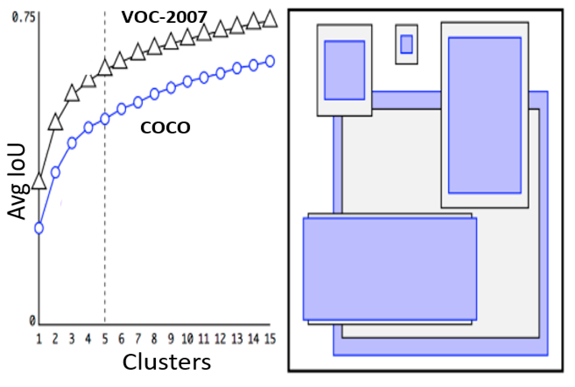
The original YOLO worked with an input image size of 224 × 224 pixels during the training stage, whilst for the detection phase, input images could be scaled up to 448 × 448 pixels, enforcing the architecture to adjust to the varying image resolution, which in turn decrease the mAP. To address this, the authors trained the architecture on 448 × 448 pixel images for 10 epochs on the ImageNet [46] dataset, providing the architecture with the capacity to adjust the internal filters when dealing with higher resolution images, resulting in an increased mAP of 4%. Whilst architectures, such as Fast and Faster R-CNN predict coordinates directly from the convolutional network, the original YOLO utilized fully connected layers to serve this purpose. YOLO-v2 replaced the fully connected layer responsible for predicting bounding boxes by adding anchor boxes for bounding box predictions. Anchor boxes [47] are essentially a list of predefined dimensions (boxes) aimed at best matching the objects of interest. Rather than manual determination of best-fit anchor boxes, the authors utilized k-means clustering [48] on the training set bounding boxes, inclusive of the ground truth bounding boxes, grouping similar shapes and plotting average IoU with respect to the closest centroid as shown in Figure 4. YOLO-v2 was trained on different architectures, namely, VGG-16 and GoogleNet, in addition to the authors proposing the Darknet-19 [49] architecture due to characteristics, such as reduced processing requirements, i.e., 5.58 FLOPs compared to 30.69 FLOPs and 8.52 FLOPs on VGG-16 and GoogleNet, respectively. In terms of performance, YOLO-v2 provided 76.8 mAP at 67 FPS and 78.6 mAP at 40 FPS. The results demonstrated the architectures’ superiority over SOTA architectures of that time, such as SSD and Faster R-CNN. YOLO-9000 utilized YOLO-v2 architecture, aimed at real-time detection of more than 9000 different objects; however, at a significantly reduced mAP of 19.7%.
2.3. YOLO-v3
Architectures, such as VGG, focused their development work around the concept that deeper networks, i.e., more internal layers, equated to higher accuracy. YOLO-v2 also had higher number of convolutional layers compared to its predecessor.
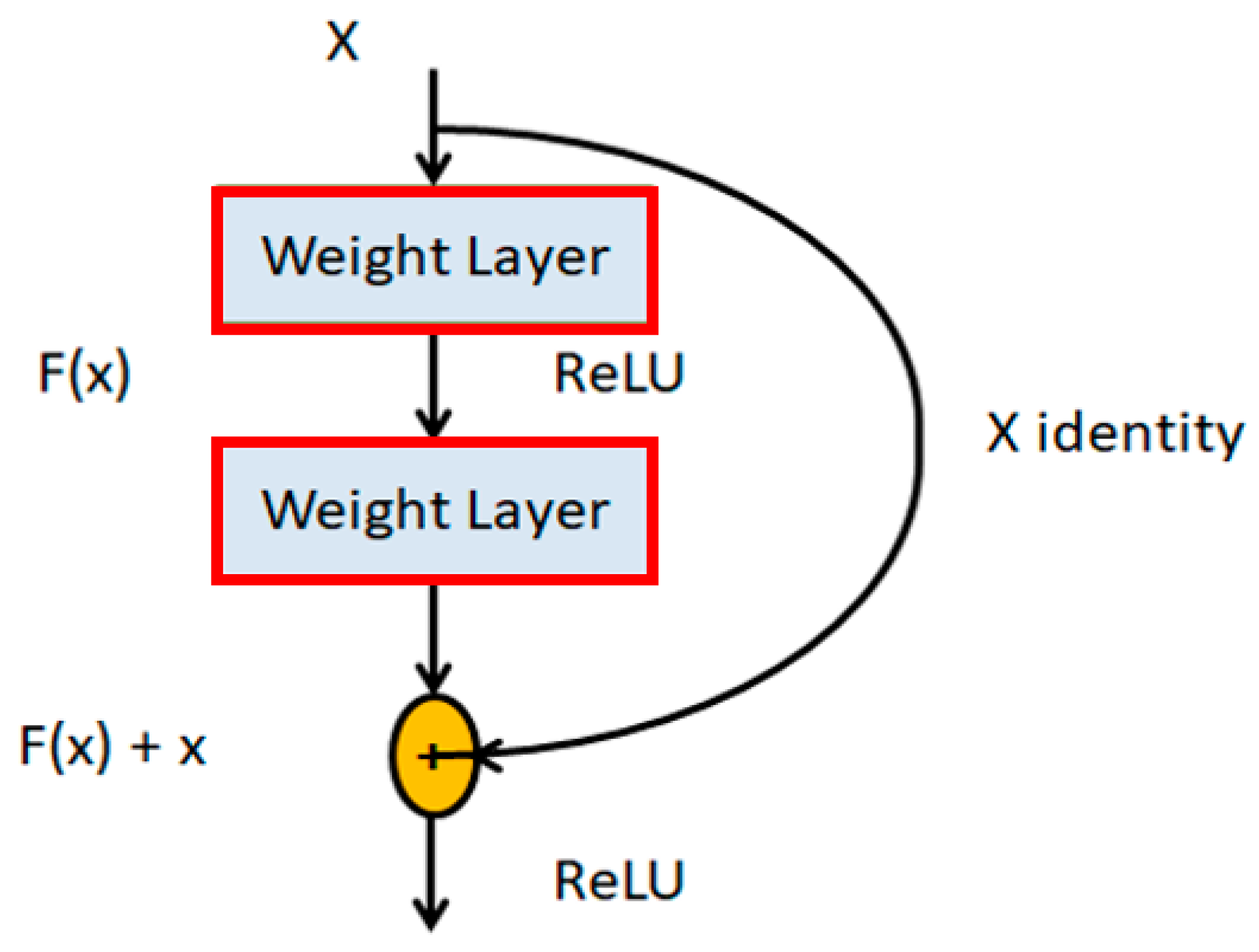
However, as the image progressed through the network, the progressive down sampling resulted in the loss of fine-grained features; therefore, YOLO-v2 often struggled with detecting smaller objects. At the time research was active in addressing this issue, as evident by the deployment of skip connections [50] embedded within the proposed ResNet architecture, the focus was on addressing the vanishing gradient issue by facilitating information propagation via skip connection, as presented in Figure 5.
YOLO-v3 proposed a hybrid architecture factoring in aspects of YOLO-v2, Darknet-53 [51], and the ResNet concept of residual networks. This enabled the preservation of fine-grained features by allowing for the gradient flow from shallow layers to deeper layers.
On top of the existing 53 layers of Darknet-53 for feature extraction, a stack of 53 additional layers was added for the detection head, totaling 106 convolutional layers for the YOLO-v3. Additionally, YOLO-v3 facilitated multi-scale detection, namely, the architecture made predictions at three different scales of granularity for outputting better performance, increasing the probability of small object detection.
2.4. YOLO-v4
YOLO-v4 was the first variant of the YOLO family after the original author discontinued further work that was introduced to the computer vision community in April 2020 by Alexey Bochkovsky et al. [52]. YOLO-v4 was essentially the distillation of a large suite of object detection techniques, tested and enhanced for providing a real-time, lightweight object detector.
The backbone of an object detector has a critical role in the quality of features extracted. In-line with the experimental spirit, the authors experimented with three different backbones: CSPResNext-50, CSPDarknet-53, and EfficientNet-B3 [53]. The first was based on DenseNet [54] aimed at alleviating the vanishing gradient problem and bolstering feature propagation and reuse, resulting in reduced number of network parameters. EfficientNet was proposed by Google Brain. The paper posits that an optima selection for parameters when scaling CNNs can be ascertained through a search mechanism. After experimenting with the above feature extractors, the authors based on their intuition and backed by their experimental results selected CSPDarknet-53 as the official backbone for YOLO-v4.
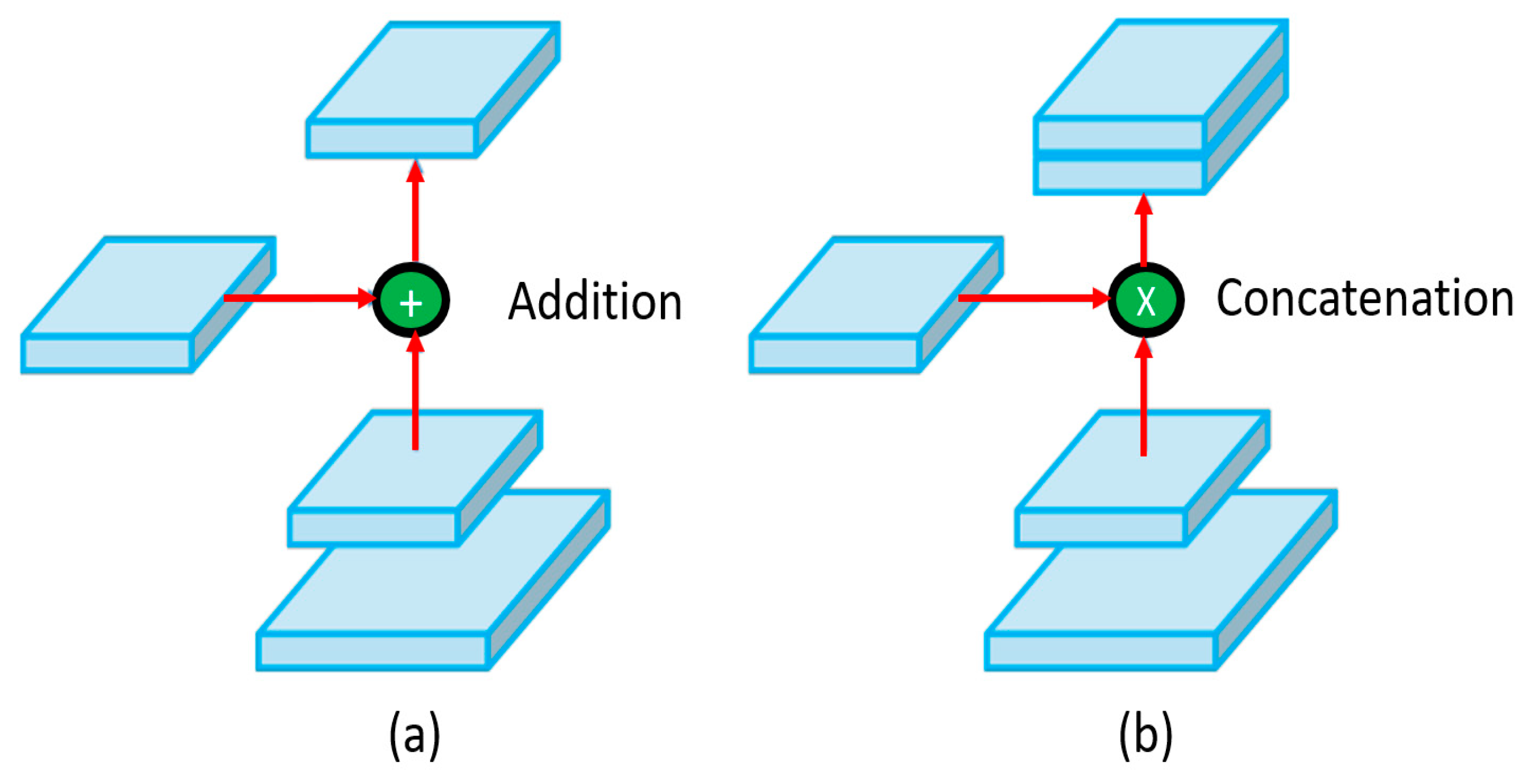
For feature aggregation, the authors experimented with several techniques for integration at the neck level including feature pyramid network (FPN) [55] and path aggregation network (PANet) [56]. Ultimately, the authors opted for PANet as the feature aggregator. The modified PANet, as shown in Figure 6, utilized the concatenation mechanism. PANet can be seen as an advanced version of FPN, namely, PANet proposed a bottom-up augmentation path along with the top-down path (FPN), adding a ‘shortcut’ connection for linking fine-grained features from high- and low-level layers. Additionally, the authors introduced a SPP [57] block post CSPDarknet-53 aimed at increasing the receptive field and separation of the important features arriving from the backbone.
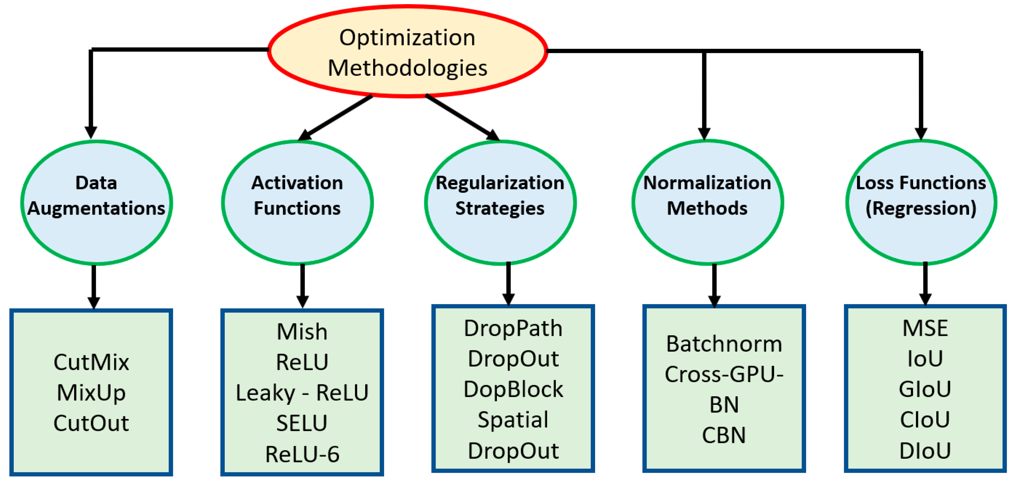
The authors also introduced a bag-of-freebies, presented in Figure 7, primarily consisting of augmentations, such as Mosaic aimed at improving performance without introducing additional baggage onto the inference time. CIoU loss [58] was also introduced as a freebie, focused on the overlap of the predicted and ground truth bounding box. In the case of no overlap, the idea was to observe the closeness of the two boxes and encourage overlap if in close proximity.
In addition to the bag-of-freebies, the authors introduced ‘bag-of-specials’, with the authors claiming that although this set of optimization techniques presented in Figure 7 would marginally impact the inference time, they would significantly improve the overall performance. One of the components within the ‘bag-of-specials’ was the Mish [59] activation function aimed at moving feature creations toward their respective optimal points. Cross mini-batch normalization [60] was also presented facilitating the running on any GPU as many batch normalization techniques involve multiple GPUs operating in tandem.
2.5. YOLO-v5
The YOLO network in essence consists of three key pillars, namely, backbone for feature extraction, neck focused on feature aggregation, and the head for consuming output features from the neck as input and generating detections. YOLO-v5 [61] similar to YOLO-v4, with respect to contributions, focus on the conglomeration and refinement of various computer vision techniques for enhancing performance. In addition, in less than 2 months after the release of YOLO-v4, Glenn Jocher open-sourced an implementation of YOLO-v5 [61].
A notable mention is that YOLO-v5 was the first native release of architectures belonging to the YOLO clan, to be written in PyTorch [62] rather than Darknet. Although Darknet is considered as a flexible low-level research framework, it was not purpose built for production environments with a significantly smaller number of subscribers due to configurability challenges. PyTorch, on the other hand, provided an established eco-system, with a wider subscription base among the computer vision community and provided the supporting infrastructure for facilitating mobile device deployment.
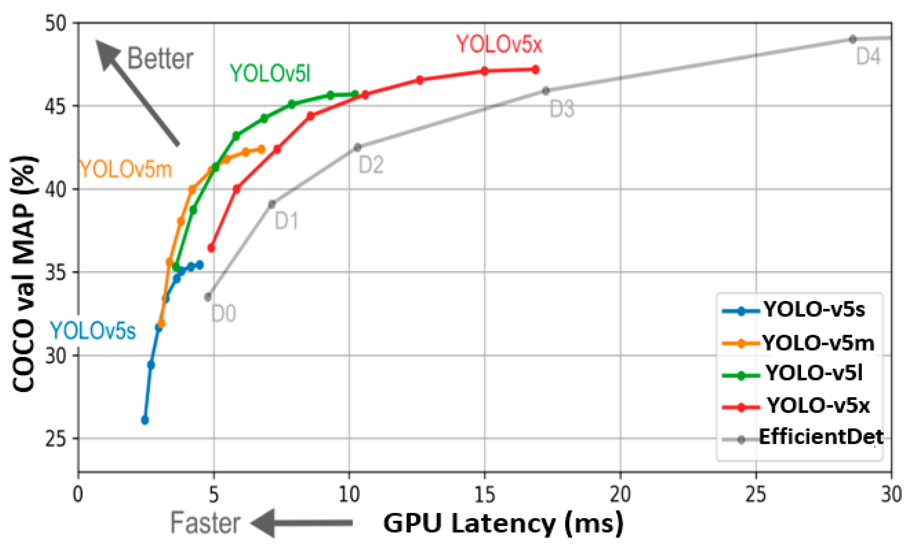
In addition, another notable proposal was the ‘automated anchor box learning’ concept. In YOLO-v2, the anchor box mechanism was introduced based on selecting anchor boxes that closely resemble the dimensions of the ground truth boxes in the training set via k-means. The authors select the five close-fit anchor boxes based on the COCO dataset [63] and implement them as default boxes. However, the application of this methodology to a unique dataset with significant object differentials compared to those present in the COCO dataset can quickly expose the inability of the predefined boxes to adapt quickly to the unique dataset. Therefore, authors in YOLO-v5 integrated the anchor box selection process into the YOLO-v5 pipeline. As a result, the network would automatically learn the best-fit anchor boxes for the particular dataset and utilize them during training to accelerate the process. YOLO-v5 comes in several variants with respect to the computational parameters as presented in Table 1.
2.6. YOLO-v6
The initial codebase for YOLO-v6 [65] was released in June 2022 by the Meituan Technical Team based in China. The authors focused their design strategy on producing an industry-orientated object detector.
To meet industrial application requirements, the architecture would need to be highly performant on a range of hardware options, maintaining high speed and accuracy. To conform with the diverse set of industrial applications, YOLO-v6 comes in several variants starting with YOLO-v6-nano as the fastest with the least number of parameters and reaching YOLO-v6-large with high accuracy at the expense of speed, as shown in Table 2.
The impressive performance presented in Table 2 is a result of several innovations integrated into the YOLO-v6 architecture. The key contributions can be summed into four points. First, in contrast to its predecessors, YOLO-v6 opts for an anchor-free approach, making it 51% faster when compared to anchor-based approaches.
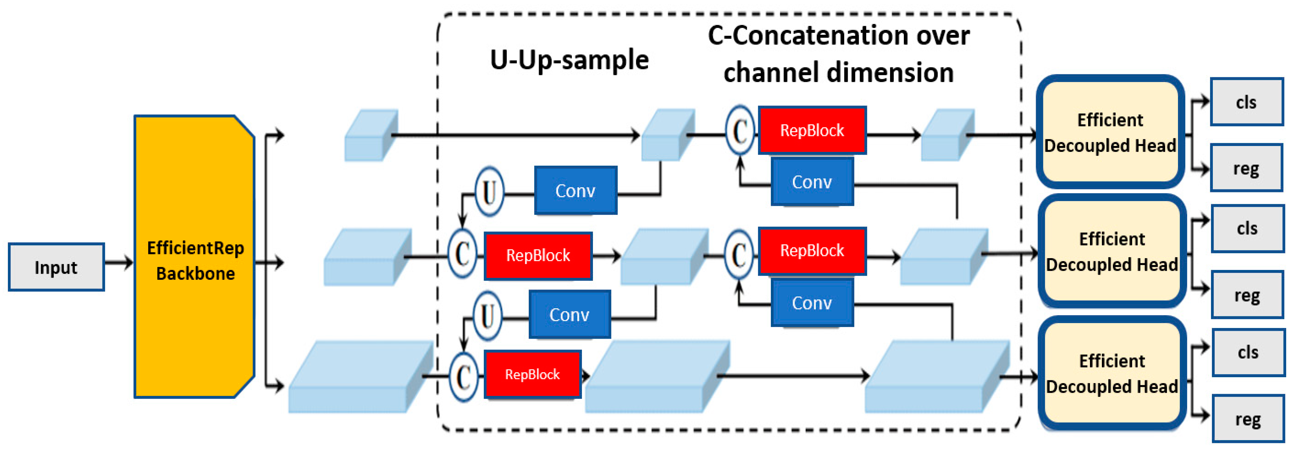
Second, the authors introduced a revised reparametrized backbone and neck, proposed as EfficientRep backbone and Rep-PAN neck [66], namely, up to and including YOLO-v5, the regression and classification heads shared the same features. Breaking the convention, YOLO-v6 implements the decoupled head as shown in Figure 9. As a result, the architecture has additional layers separating features from the final head, as empirically shown to improve the performance. Third, YOLO-v6 mandates a two-loss function. Varifocal loss (VFL) [67] is used as the classification loss and distribution focal loss (DFL) [68], along with SIoU/GIoU [69] as regression loss. VFL being a derivative of focal loss, treats positive and negative samples at varying degrees of importance, helping in balancing the learning signals from both sample types. DFL is deployed for box regression in YOLO-v6 medium and large variants, treating the continuous distribution of the box locations as discretized probability distribution, which is shown to be particularly efficient when the ground truth box boundaries are blurred.
Additional improvements focused on industrial applications include the use of knowledge distillation [70], involving a teacher model used for training a student model, where the predictions of the teacher are used as soft labels along with the ground truth for training the student. This comes without fueling the computational cost as essentially the aim is to train a smaller (student) model to replicate the high performance of the larger (teacher) model. Comparing the performance of YOLO-v6 with its predecessors, including YOLO-v5 on the benchmark COCO dataset in Figure 10, it is clear that YOLO-v6 achieves a higher mAP at various FPS.
2.7. YOLO-v7
The following month after the release of YOLO-v6, the YOLO-v7 was released [72]. Although other variants have been released in between, including YOLO-X [73] and YOLO-R [74], these focused more on GPU speed enhancements with respect to inferencing. YOLO-v7 proposes several architectural reforms for improving the accuracy and maintaining high detection speeds. The proposed reforms can be split into two categories: Architectural reforms and Trainable BoF (bag-of-freebies). Architectural reforms included the implementation of the E-ELAN (extended efficient layer aggregation network) [75] in the YOLO-v7 backbone, taking inspiration from research advancements in network efficiency. The design of the E-ELAN was guided by the analysis of factors that impact accuracy and speed, such as memory access cost, input/output channel ratio, and gradient path.
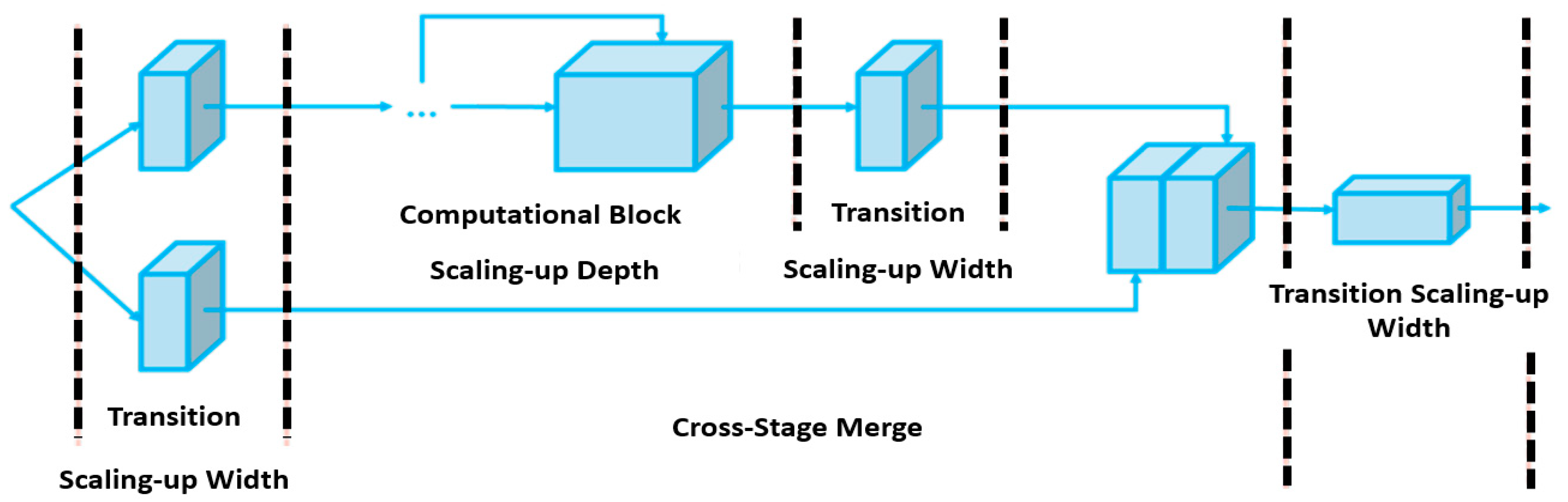
The second architectural reform was presented as compound model scaling, as shown in Figure 11. The aim was to cater for a wider scope of application requirements, i.e., certain applications require accuracy to be prioritized, whilst others may prioritize speed. Although NAS (network architecture search) [76] can be used for parameter-specific scaling to find the best factors, the scaling factors are independent [77]. Whereas the compound-scaling mechanism allows for the width and depth to be scaled in coherence for concatenation-based networks, maintaining optimal network architecture while scaling for different sizes.
Re-parameterization planning is based on averaging a set of model weights to obtain a more robust network [78,79]. Expanding further, module level re-parameterization enables segments of the network to regulate their own parameterization strategies. YOLO-v7 utilizes gradient flow propagation paths with the aim to observe which internal network modules should deploy re-parameterization strategies.
The auxiliary head coarse-to-fine concept is proposed on the premise that the network head is quite far downstream; therefore, the auxiliary head is deployed at the middle layers to assist in the training process. However, this would not train as efficiently as the lead head, due to the former not having access to the complete network.
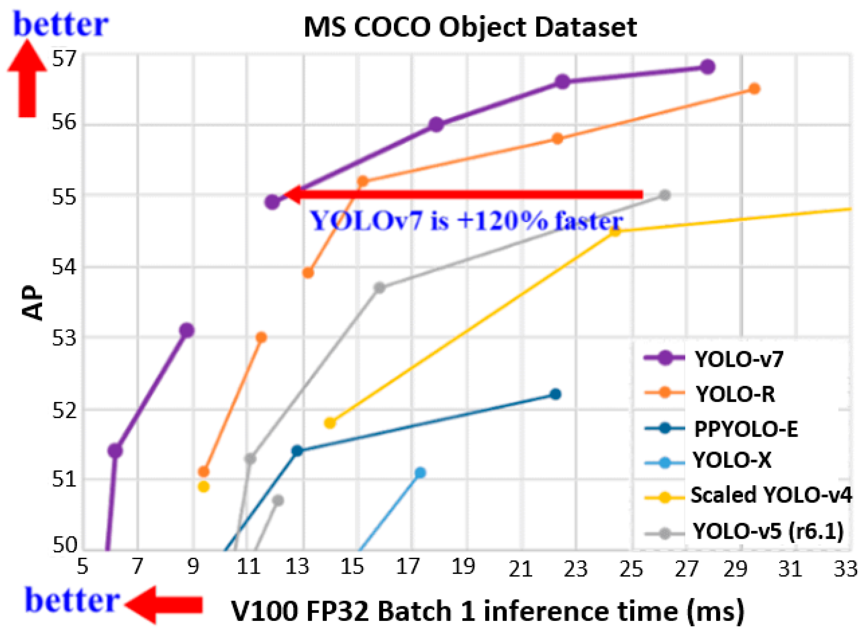
Figure 12 presents a performance comparison of YOLO-v7 with the preceding YOLO variants on the MS COCO dataset. It is clear from Figure 12 that all YOLO-v7 variants surpassed the compared object detectors in accuracy and speed in the range of 5–160 FPS. It is, however, important to note, as mentioned by the authors of YOLO-v7, that none of the YOLO-v7 variants are designed for CPU-based mobile device deployment. YOLO-v7-tiny/v7/W6 variants are designed for edge GPU, consumer GPU, and cloud GPU, respectively. Whilst YOLO-v7-E6/D6/E6E are designed for high-end cloud GPUs only.
Internal variant comparison of YOLO-v7 is presented in Table 3. As evident, there is a significant performance gap with respect to mAP when comparing YOLO-v7-tiny with the computationally demanding YOLO-v7-D6. However, the latter would not be suitable for edge deployment onto a computationally constrained device.
2.8. YOLO-v8
The latest addition to the family of YOLO was confirmed in January 2023 with the release of YOLO-v8 [80] by Ultralytics (also released YOLO-v5). Although a paper release is impending and many features are yet to be added to the YOLO-v8 repository, initial comparisons of the newcomer against its predecessors demonstrate its superiority as the new YOLO state-of-the-art.
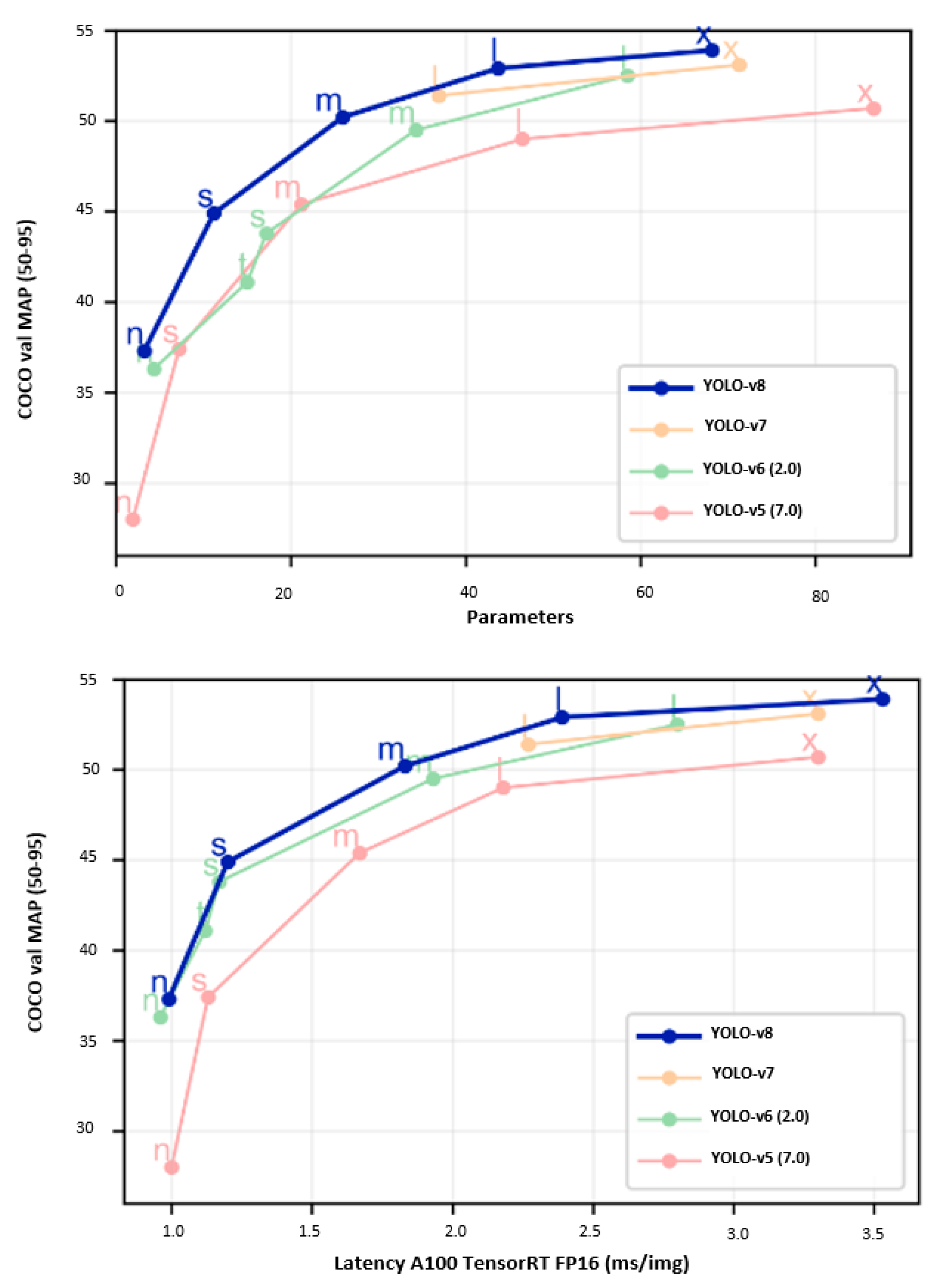
Figure 13 demonstrates that when comparing YOLO-v8 against YOLO-v5 and YOLO-v6 trained on 640 image resolution, all YOLO-v8 variants output better throughput with a similar number of parameters, indicating toward hardware-efficient, architectural reforms. The fact that YOLO-v8 and YOLO-v5 are presented by Ultralytics with YOLO-v5 providing impressive real-time performance and based on the initial benchmarking results released by Ultralytics, it is strongly assumed that the YOLO-v8 will be focusing on constrained edge device deployment at high-inference speed.
3. Industrial Defect Detection via YOLO
The previous section demonstrates the rapid evolution of the YOLO ‘clan’ of object detectors amongst the computer vision community. This section of the review focuses on the implementation of YOLO variants for the detection of surface defects within the industrial setting. The selection of ‘industrial setting’ is due to its varying and stringent requirements alternating between accuracy and speed, a theme which is found through DNA of the YOLO variants.
3.1. Industrial Fabric Defect Detection
Rui Jin et al. [81] in their premise state the inefficiencies of manual inspection in the textile manufacturing domain as high cost of labor, human-related fatigue, and reduced detection speed (less than 20 m/min). The authors aim to address these inefficiencies by proposing a YOLO-v5-based architecture, coupled with a spatial attention mechanism for accentuation of smaller defective regions. The proposed approach involved a teacher network trained on the fabric dataset. Post training of the teacher network, the learned weights were distilled to the student network, which was compatible for deployment onto a Jetson TX2 [82] via TensorRT [83]. The results presented by the authors show, as expected, that the teacher network reported higher performance with an AUC of 98.1% compared to 95.2% (student network). However, as the student network was computationally smaller, the inference time was significantly less at 16 ms for the student network in contrast to the teacher network at 35 ms on the Jetson TX2. Based on the performance, the authors claim that the proposed solution provides high accuracy and real-time inference speed, making it compatible for deployment via the edge device.
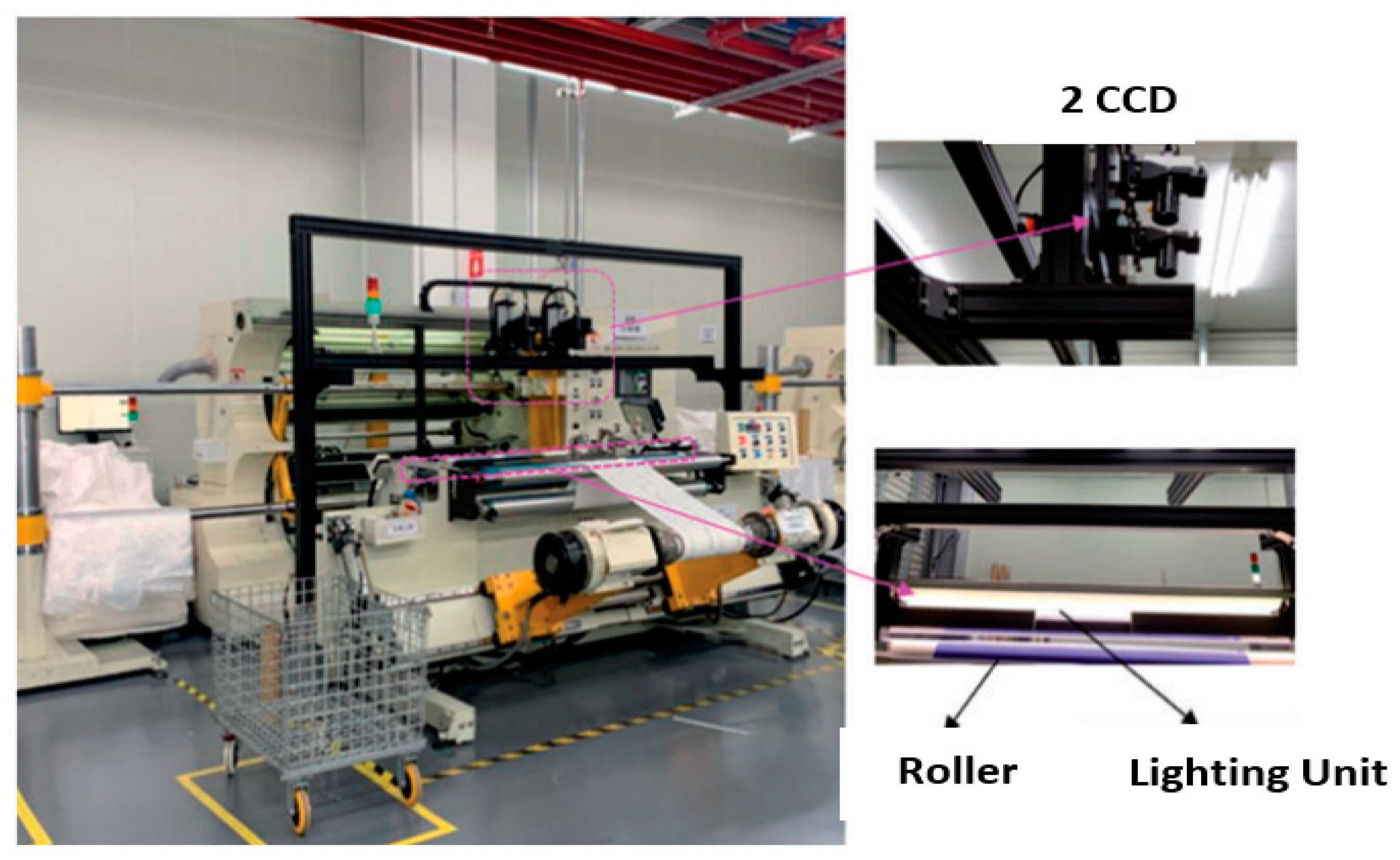
Sifundvoleshile Dlamini et al. [84] propose a production environment fabric defect detection framework focused on real-time detection and accurate classification on-site, as shown in Figure 14. The authors embed conventional image processing at the onset of their data enhancement strategy, i.e., filtering to denoise feature enhancement. Post augmentations and data scaling, the authors train the YOLO-v4 architecture based on pretrained weights. The reported performance was respectable with an F1-score of 93.6%, at an impressive detection speed of 34 fps and prediction speed of 21.4 ms. The authors claim that the performance is evident to the effectiveness of the selected architecture for the given domain.
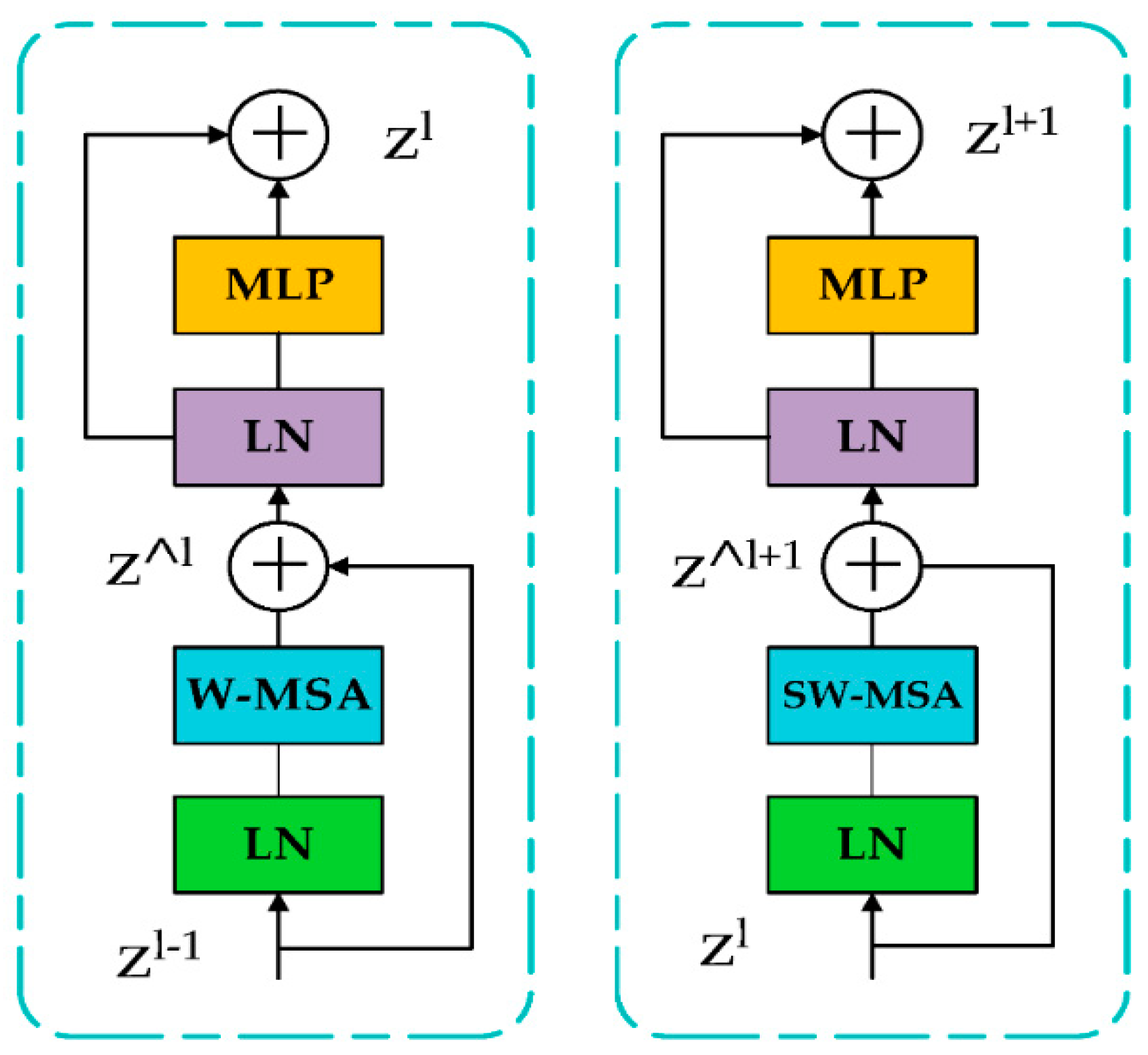
Restricted by the available computing resources for edge deployment, Guijuan Lin et al. [85] state problems with quality inspection in the fabric production domain, including minute scale of defects, extreme unbalance with the aspect ratio of certain defects, and slow defect detection speeds. To address these issues, the authors proposed a sliding-window, self-attention (multihead) mechanism calibrated for small defect targets. Additionally, the Swin Transformer [86] module as depicted in Figure 15 was integrated into the original YOLO-v5 architecture for the extraction of hierarchical features. Furthermore, the generalized focal loss is implemented with the architecture aimed at improving the learning process for positive target instances, whilst lowering the rate of missed detections. The authors report the accuracy of the proposed solution on a real-world fabric dataset, reaching 76.5% mAP at 58.8 FPS, making it compatible with the real-time detection requirements for detection via embedded devices.
3.2. Solar Cell Surface Defect Detection
Setting their premise, the authors [87] state that human-led Photovoltaic (PV) inspection has many drawbacks including the requirement of operation and maintenance (O&M) engineers, cell-by-cell inspection, high workload, and reduced efficiency. The authors propose an improved architecture based on YOLO-v5 for the characterization of complex solar cell surface textures and defective regions. The proposal is based on the integration of deformable convolution within the CSP module with the aim of achieving an adaptive learning scale. Additionally, an attention mechanism is incorporated for enhanced feature extraction. Moreover, the authors optimize the original YOLO-v5 architecture further via K-means++ clustering for anchor box determination algorithm. Based on the presented results, the improved architecture achieved a respectable mAP of 89.64% on an EL-based solar cell image dataset, 7.85% higher compared to mAP for the original architecture, with detection speed reaching 36.24 FPS, which can be translated as a more accurate detection while remaining compatible with the real-time requirements.
Amran Binomairah et al. [88] highlight two frequent defects encountered during the manufacturing process of crystalline solar cells as dark spot/region and microcracks. The latter can have a detrimental impact on the performance of the module, which is a major cause for PV module failures. The authors subscribe to the YOLO architecture, comparing the performance of their methodology on YOLO-v4 and an improved YOLO-v4-tiny integrated with a spatial pyramid pooling mechanism. Based on the presented results, YOLO-v4 achieved 98.8% mAP at 62.9 ms, whilst the improved YOLO-v4-tiny lagged with 91% mAP at 28.2 ms. The authors claim that although the latter is less accurate, it is notably faster than the former.
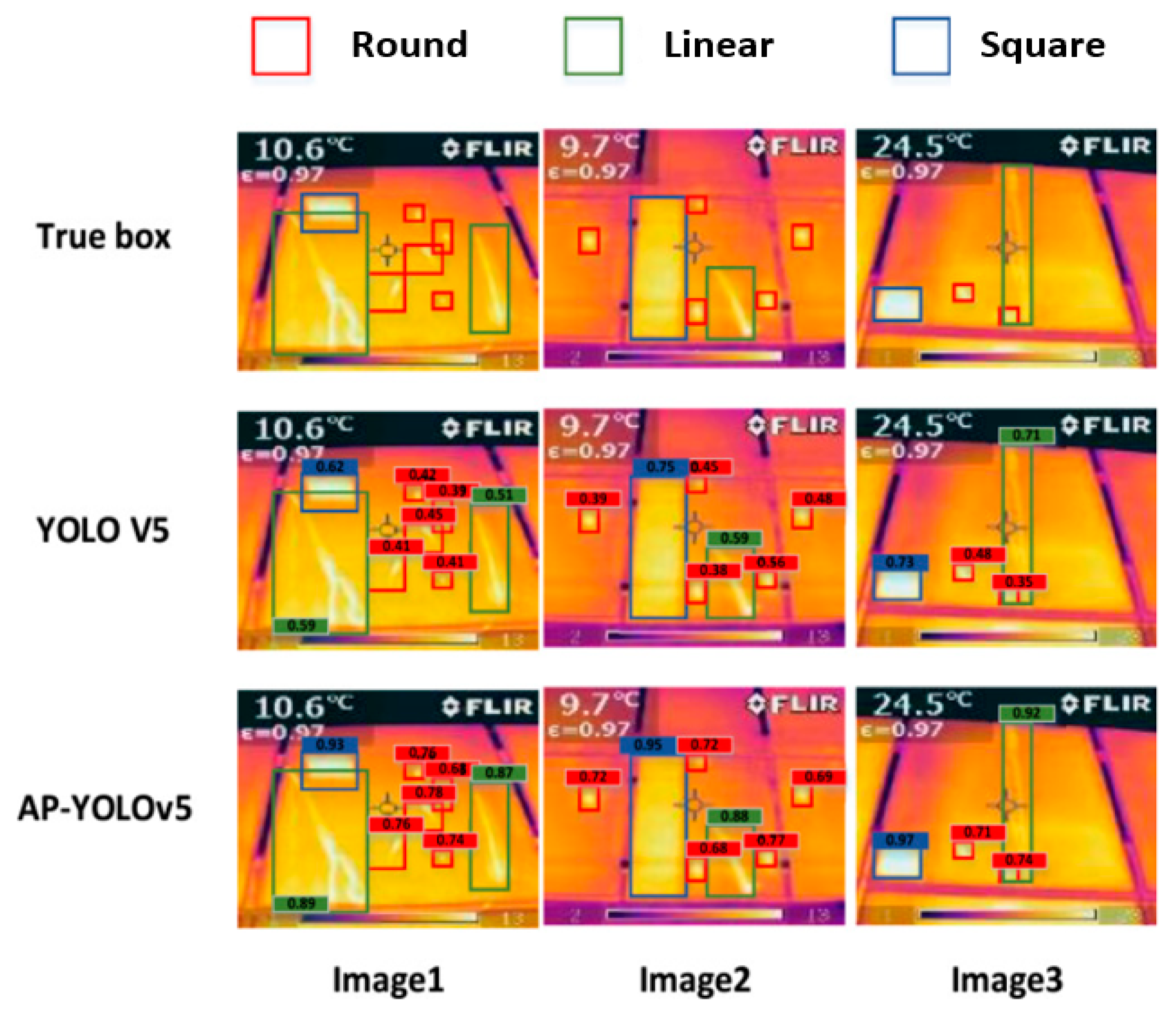
Tianyi Sun et al. [89] focus on automated hot-spot detection within PV cells based a modified version of the YOLO-v5 architecture. The first improvement comes in the form of enhanced anchors and detection heads for the respective architecture. To improve the detection precision at varying scales, k-means clustering [48] is deployed for clustering the length–width ratio with respect to the data annotation frame. Additionally, a set of the anchors consisting of smaller values were added to cater for the detection of small defects by optimizing the cluster number. The reported performance of the improved architecture was reported as 87.8% mAP, with the average recall rate of 89.0% and F1-score reaching 88.9%. The reported FPS was impressive reaching 98.6 FPS, with the authors claiming that the proposed solution would provide intelligent monitoring at PV power stations. Inferencing output presented in Figure 16 shows the proposed AP-YOLO-v5 architecture, providing inferences at a higher confidence level compared to the original YOLO-v5.
3.3. Steel Surface Defect Detection
Dinming Yang et al. [90] set the premise of their research by stating the importance of steel pipe quality inspection, citing the growing demand in countries, such as China. Although X-ray testing is utilized as one of the key methods for industrial nondestructive testing (NDT), the authors state that it still requires human assistance for the determination, classification, and localization of the defects. The authors propose the implementation of YOLO-v5 for production-based weld steel defect detection based on X-ray images of the weld pipe. The authors claim that the trained YOLO-v5 reached a mAP of 98.7% (IoU-0.5), whilst meeting the real-time detection requirements of steel pipe production with a single image detection rate of 0.12 s.
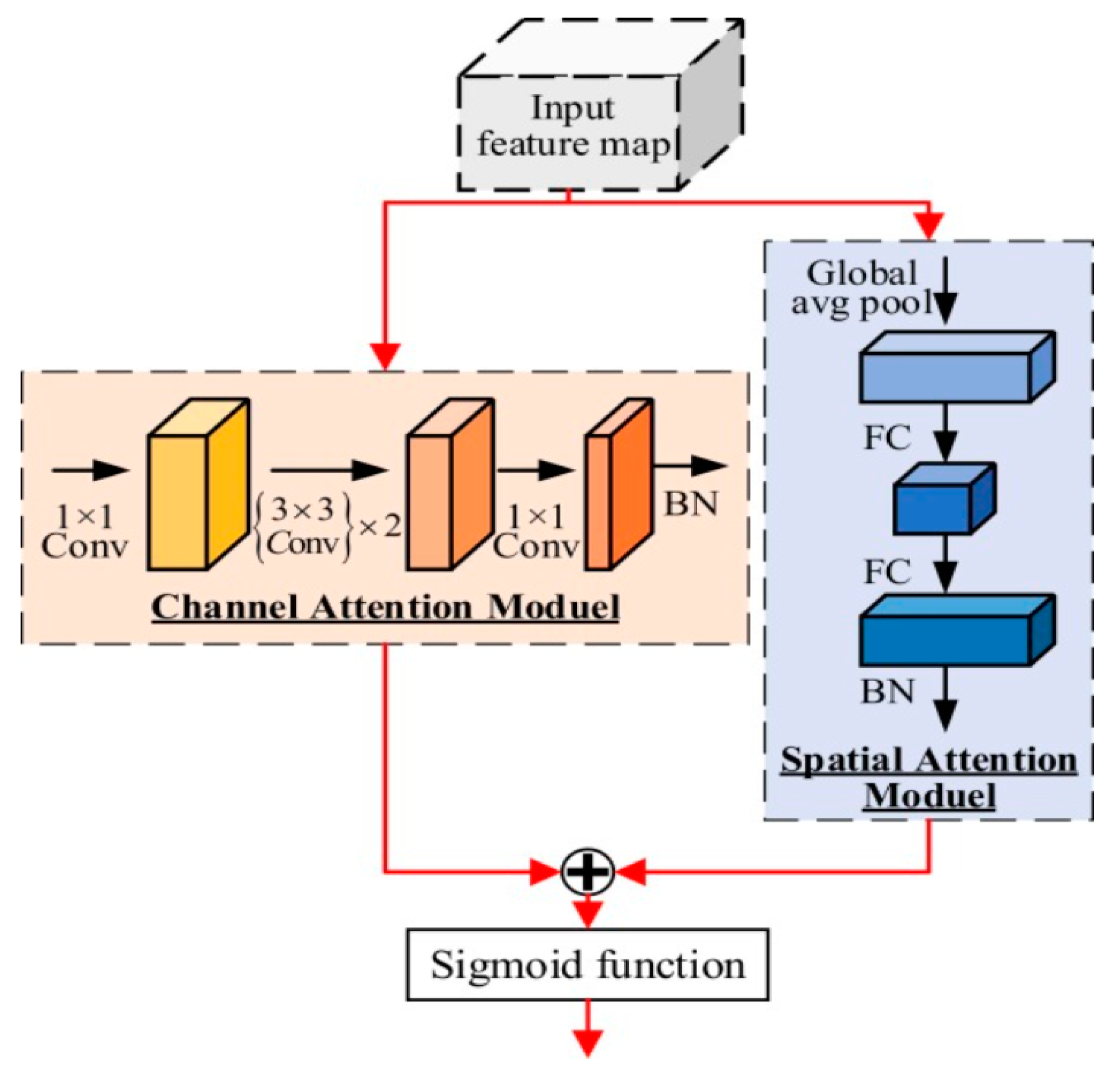
Zhuxi MA et al. [91] address the issue of large-scale computation and specific hardware requirements for automated defect detection in aluminum strips. The authors select YOLO-v4 as the architecture, whilst the backbone is constructed to make use of depth-wise separable convolutions along with a parallel dual attention mechanism for feature enhancement, as shown in Figure 17. The proposed network is tested on real data from a cold-rolling workshop, providing impressive results on real data achieving an mAP of 96.28%. Compared to the original YOLO-v4, the authors claim that the proposed architecture volume is reduced by 83.38%, whilst the inference speed is increased by a factor of three. The increase in performance was partly due to the custom anchor approach, whereby due to the maximum aspect ratio of the custom dataset, the defect was set to 1:20 which is in-line with the defect characteristics, such as scratch marks.
Jianting Shi et al. [92] cite the manufacturing process of steel production as the reason for various defects originating on the steel surface, such as rolling scale and patches. The authors state that the small dimensions of the defects as well as the stringent detection requirements make the quality inspection process a challenging task. Therefore, the authors present an improved version of YOLO-v5 by incorporating an attention mechanism for facilitating the transmission of shallow features from the backbone to the neck, preserving the defective regions, in addition to k-means clustering of anchor boxes for addressing the extreme aspect ratios of defective targets within the dataset. The authors state that the improved architecture achieved 86.35% mAP reaching 45 FPS detection speed, whilst the original architecture achieved 81.78% mAP at 52 FPS.
3.4. Pallet Racking Defect Inspection
A promising application with significant deployment scope in the warehousing and general industrial storage centers is automated pallet racking inspection. Warehouses and distribution centers host a critical infrastructure known as racking for stock storage. Unnoticed damage to pallet racking can pave the way for significant losses initiated by racking collapse leading to wasted/damaged stock, financial implications, operational losses, injured employees, and worst-case, loss of lives [93]. Due to the inefficiencies of the conventional racking inspection mechanisms, such as human-led annual inspection resulting in labor costs, bias, fatigue, and mechanical products, such as rackguards [94] lacking classification intelligence, CNN-based automated detection seems to be a promising alternative.
Realizing the potential, Hussain et al. [95] inaugurated research into automated pallet racking detection via computer vision. After presenting their initial research based on the MobileNet-V2 architecture, the authors recently proposed the implementation of YOLO-v7 for automated pallet racking inspection [96]. The selection of the architecture was in-line with the stringent requirements of production floor deployment, i.e., edge device deployment, placed onto an operating forklift, requiring real-time detection as the forklift approaches the racking. Evaluating the performance of the proposed solution on a real dataset, the authors claimed an impressive performance of 91.1% mAP running at 19 FPS.
Table 4 presents a comparison of the present research in this emerging field. Although mask R-CNN presents the highest accuracy, which is a derivative of the segmentation family of architectures with significant computational load, this makes it an infeasible option for deployment. Whereas the proposed approach utilizing YOLO-v7 achieved similar accuracy compared to MobileNet-V2, whilst requiring significantly less training data along with inferencing at 19 FPS.
4. Discussion
The YOLO family of object detectors has had a significant impact on improving the potential of computer vision applications. Right from the onset, i.e., the release of the YOLO-v1 in 2015, significant breakthroughs were introduced. YOLO-v1 became the first architecture combining the two conventionally separate tasks of bounding box prediction and classification into one. YOLO-v2 was released in the following year, introducing architectural improvements and iterative improvements, such as batch normalization, higher resolution, and anchor boxes. In 2018, YOLO-v3 was released, an extension of previous variants with enhancements including the introduction of objectness scores for bounding box predictions added connections for the backbone layers and the ability to generate predictions at three different levels of granularity, leading to improved performance on smaller object targets.
After a short delay, YOLO-v4 was released in April 2020, becoming the first variant of the YOLO family not to be authored by the original author Joseph Redmon. Enhancements included improved feature aggregation, gifting of the ‘bag of freebies’, and the mish activation. In a matter of months, YOLO-v5 entered the computer vision territory, becoming the first variant to be released without being accompanied by a paper release. YOLO-v5 based on PyTorch, with an active GitHub repo further delineated the implementation process, make it accessible to a wider audience. Focused on internal architectural reforms, YOLO-v6 authors redesigned the backbone (EfficientRep) and neck (Rep-PAN) modules, with an inclination toward hardware efficiency. Additionally, anchor-free and the concept of decoupled head was introduced, implying additional layers for feature separation from the final head, which is empirically shown to improve the overall performance. The authors of YOLO-v7 also focused on architectural reforms, considering the amount of memory required to keep layers within memory and the distance required for gradients to back-propagate, i.e., shorter gradients, resulting in enhanced learning capacity. For the ultimate layer aggregation, the authors implemented E-ELAN, which is an extension of the ELAN computational block. The advent of 2023 introduced the latest version of the YOLO family, YOLO-v8, which was released by Ultralytics. With an impending paper release, initial comparisons of the latest version against predecessors have shown promising performance with respect to throughput when compared to similar computational parameters.
4.1. Reason for Rising Popularity
Table 5 presents a summary of the reviewed YOLO variants based on the underlying framework, backbone, average-precision (AP), and key contributions. It can be observed from Table 3 that as the variants evolved there was a shift from the conservative Darknet framework to a more accessible one, i.e., PyTorch. The AP presented here is based on COCO-2017 [63] with the exception of YOLO-v1/v2, which are based on VOC-2017 [39]. COCO-2017 [63] consists of over 80 objects designed to represent a vast array of regularly seen object. It contains 121,408 images resulting in 883,331 object annotations with median image ratio of 640 × 480 pixels. It is important to note that the overall accuracy along with inference capacity depends on the deployed design/training strategies, as demonstrated in the industrial surface detection section.
The AP metric consists of precision-recall (PR) metrics, defining of a positive prediction using Intersection over Union, and the handling of multiple object categories. AP provides a balanced overview of PR based on the area under the PR curve. IoU facilitates the quantification of similarity between predicted and ground truth bounding boxes as expressed in (8):
The rise of YOLO can be attributed to two factors. First, the fact that the architectural composition of YOLO variants is compatible for one-stage detection and classification makes it computationally lightweight with respect to other detectors. However, we feel that efficient architectural composition by itself did not drive the popularity of the YOLO variants, as other single-stage detectors, such as MobileNets, also serve a similar purpose.
The second reason is the accessibility factor, which was introduced as the YOLO variants progressed, with YOLO-v5 being the turning point. Expanding further on this point, the first two variants were based on the Darknet framework. Although this provided a degree of flexibility, accessibility was limited to a smaller user base due to the required expertise. Ultralytics, introduced YOLO-v5 based on the PyTorch framework, making the architecture available for a wider audience and increasing the potential domain of applications.
As evident from Table 6, the migration to a more accessible framework coupled with architectural reforms for improved real-time performance sky-rocketed. At present, YOLO-v5 has 34.7 k stars, a significant lead compared to its predecessors. From implementation, YOLO-v5 only required the installation of lightweight python libraries. The architectural reforms indicated that the model training time was reduced, which in turn reduced the experimentation cost attributed to the training process, i.e., GPU utilization. For deployment and testing purposes, researchers have several routes, such as individual/batch images, video/webcam feeds, in addition to simple weight conversion to ONXX weights for edge device deployment.
4.2. YOLO and Industrial Defect Detection
Manifestations of the fourth industrial revolution can be observed at present in an ad-hoc manner, spanning across various industries. With respect to the manufacturing industry, this revolution can be targeted at the quality inspection processes, which are vital for assuring efficiency and retaining client satisfaction. When focusing on surface defect detection, as alluded to earlier, the inspection requirements can be more stringent as compared to other applications. This is due to many factors, such as the fact that the defects may be extremely small, requiring external spectral imaging to expose defects prior to classification and due to the fact that the operational setting of the production line may only provide a small-time window within which inference must be carried out.
Considering the stringent requirements outlined above and benchmarking against the principles of YOLO family of variants, forms the conclusion that the YOLO variants have the potential to address both real-time, constrained deployment and small-scale defect detection requirements of industrial-based surface defect detection. YOLO variants have proven real-time compliance in several industrial environments as shown in [81,84,85,90,95]. An interesting observation arising from the industrial literature reviewed is the ability for users to modify the internal modules of YOLO variants in order to take care of their specific application needs without compromising on real-time compliance, for example [81,87,91,92], introducing attention-mechanisms for accentuation of defective regions.
An additional factor, found within the later YOLO variants is sub-variants for each base architecture, i.e., for YOLO-v5 variants including YOLO-v5-S/M/L, this corresponds to different computational loads with respect to the number of parameters. This flexibility enables researchers to consider a more flexible approach with the architecture selection criteria based on the industrial requirements, i.e., if real-time inference is required with less emphasis on optimal mAP, a lightweight variant can be selected, such as YOLO-v5-small rather than YOLO-v5-large.
5. Conclusions
In conclusion, this work is the first of its type focused on documenting and reviewing the evolution of the most prevalent single-stage object detector within the computer vision domain. The review presents the key advancements of each variant, followed by implementation of YOLO architectures within various industrial settings focused on surface automated real-time surface defect detection.
From the review, it is clear as the YOLO variants have progressed, latter versions in particular, YOLO-v5 has focused on constrained edge deployment, a key requirement for many manufacturing applications. Due to the fact that there is no copyright and patent restrictions, research anchored around the YOLO architecture, i.e., real-time, lightweight, accurate detection, can be conducted by any individual or research organization, which has also contributed to the prevalence of this variant.
With YOLO-v8 released in January 2023, showing promising performance with respect to throughput and computational load requirements, it is envisioned that 2023 will see more variants released by previous or new authors focused on improving the deployment capacity of the architectures with respect to constrained deployment environments.
With research organizations, such as Ultralytics and Meituan Technical Team taking a keen interest in the development of YOLO architectures with a focus on edge-friendly deployment, we anticipate further technological advancements in the architectural footprint of YOLO. To cater for constrained deployment, these advancements will need to focus on energy conservation whilst maintaining high inference rates. Furthermore, we envision the proliferation of YOLO architectures into production facilities to help with quality inspection pipelines as well as providing stimulus for innovative products as demonstrated by [96] with an automated pallet racking inspection solution. Along with integration into a diverse set of hardware and IoT devices, YOLO has the potential to tap into new domains where computer vision can assist in enhancing existing processes whilst requiring limited resources.
Funding
This research received no external funding.
Data Availability Statement
Not applicable.
Conflicts of Interest
The authors declare no conflict of interest.
References
- Zhang, B.; Quan, C.; Ren, F. Study on CNN in the recognition of emotion in audio and images. In Proceedings of the 2016 IEEE/ACIS 15th International Conference on Computer and Information Science (ICIS), Okayama, Japan, 26–29 June 2016. [Google Scholar] [CrossRef]
- Pollen, D.A. Explicit neural representations, recursive neural networks and conscious visual perception. Cereb. Cortex 2003, 13, 807–814. [Google Scholar] [CrossRef] [PubMed] [Green Version]
- Using artificial neural networks to understand the human brain. Res. Featur. 2022. [CrossRef]
- Improvement of Neural Networks Artificial Output. Int. J. Sci. Res. (IJSR) 2017, 6, 352–361. [CrossRef]
- Dodia, S.; Annappa, B.; Mahesh, P.A. Recent advancements in deep learning based lung cancer detection: A systematic review. Eng. Appl. Artif. Intell. 2022, 116, 105490. [Google Scholar] [CrossRef]
- Ojo, M.O.; Zahid, A. Deep Learning in Controlled Environment Agriculture: A Review of Recent Advancements, Challenges and Prospects. Sensors 2022, 22, 7965. [Google Scholar] [CrossRef] [PubMed]
- Jarvis, R.A. A Perspective on Range Finding Techniques for Computer Vision. IEEE Trans. Pattern Anal. Mach. Intell. 1983, PAMI-5, 122–139. [Google Scholar] [CrossRef]
- Hussain, M.; Bird, J.; Faria, D.R. A Study on CNN Transfer Learning for Image Classification. 11 August 2018. Available online: https://research.aston.ac.uk/en/publications/a-study-on-cnn-transfer-learning-for-image-classification (accessed on 1 January 2023).
- Yang, R.; Yu, Y. Artificial Convolutional Neural Network in Object Detection and Semantic Segmentation for Medical Imaging Analysis. Front. Oncol. 2021, 11, 638182. [Google Scholar] [CrossRef]
- Haupt, J.; Nowak, R. Compressive Sampling vs. Conventional Imaging. In Proceedings of the 2006 International Conference on Image Processing, Las Vegas, NV, USA, 26–29 June 2006; pp. 1269–1272. [Google Scholar] [CrossRef]
- Gu, J.; Wang, Z.; Kuen, J.; Ma, L.; Shahroudy, A.; Shuai, B.; Liu, T.; Wang, X.; Wang, G.; Cai, J.; et al. Recent advances in convolutional neural networks. Pattern Recognit. 2018, 77, 354–377. [Google Scholar] [CrossRef] [Green Version]
- Perez, H.; Tah, J.H.M.; Mosavi, A. Deep Learning for Detecting Building Defects Using Convolutional Neural Networks. Sensors 2019, 19, 3556. [Google Scholar] [CrossRef] [Green Version]
- Hussain, M.; Al-Aqrabi, H.; Hill, R. PV-CrackNet Architecture for Filter Induced Augmentation and Micro-Cracks Detection within a Photovoltaic Manufacturing Facility. Energies 2022, 15, 8667. [Google Scholar] [CrossRef]
- Hussain, M.; Dhimish, M.; Holmes, V.; Mather, P. Deployment of AI-based RBF network for photovoltaics fault detection procedure. AIMS Electron. Electr. Eng. 2020, 4, 1–18. [Google Scholar] [CrossRef]
- Hussain, M.; Al-Aqrabi, H.; Munawar, M.; Hill, R.; Parkinson, S. Exudate Regeneration for Automated Exudate Detection in Retinal Fundus Images. IEEE Access 2022. [Google Scholar] [CrossRef]
- Hussain, M.; Al-Aqrabi, H.; Hill, R. Statistical Analysis and Development of an Ensemble-Based Machine Learning Model for Photovoltaic Fault Detection. Energies 2022, 15, 5492. [Google Scholar] [CrossRef]
- Singh, S.A.; Desai, K.A. Automated surface defect detection framework using machine vision and convolutional neural networks. J. Intell. Manuf. 2022, 34, 1995–2011. [Google Scholar] [CrossRef]
- Weichert, D.; Link, P.; Stoll, A.; Rüping, S.; Ihlenfeldt, S.; Wrobel, S. A review of machine learning for the optimization of production processes. Int. J. Adv. Manuf. Technol. 2019, 104, 1889–1902. [Google Scholar] [CrossRef]
- Wang, J.; Ma, Y.; Zhang, L.; Gao, R.X.; Wu, D. Deep learning for smart manufacturing: Methods and applications. J. Manuf. Syst. 2018, 48, 144–156. [Google Scholar] [CrossRef]
- Weimer, D.; Scholz-Reiter, B.; Shpitalni, M. Design of deep convolutional neural network architectures for automated feature extraction in industrial inspection. CIRP Ann. 2016, 65, 417–420. [Google Scholar] [CrossRef]
- Kusiak, A. Smart manufacturing. Int. J. Prod. Res. 2017, 56, 508–517. [Google Scholar] [CrossRef]
- Yang, J.; Li, S.; Wang, Z.; Dong, H.; Wang, J.; Tang, S. Using Deep Learning to Detect Defects in Manufacturing: A Comprehensive Survey and Current Challenges. Materials 2020, 13, 5755. [Google Scholar] [CrossRef]
- Soviany, P.; Ionescu, R.T. Optimizing the Trade-Off between Single-Stage and Two-Stage Deep Object Detectors using Image Difficulty Prediction. In Proceedings of the 2018 20th International Symposium on Symbolic and Numeric Algorithms for Scientific Computing (SYNASC), Timisoara, Romania, 20–23 September 2018. [Google Scholar] [CrossRef]
- Du, L.; Zhang, R.; Wang, X. Overview of two-stage object detection algorithms. J. Phys. Conf. Ser. 2020, 1544, 012033. [Google Scholar] [CrossRef]
- Sultana, F.; Sufian, A.; Dutta, P. A Review of Object Detection Models Based on Convolutional Neural Network. In Advances in Intelligent Systems and Computing; Springer: Singapore, 2020; pp. 1–16. [Google Scholar] [CrossRef]
- Liu, W.; Anguelov, D.; Erhan, D.; Szegedy, C.; Reed, S.; Fu, C.Y.; Berg, A.C. SSD: Single shot multibox detector. In Proceedings of the Computer Vision—ECCV 2016, Amsterdam, The Netherlands, 11–14 October 2016; pp. 21–37. [Google Scholar] [CrossRef] [Green Version]
- Fu, C.Y.; Liu, W.; Ranga, A.; Tyagi, A.; Berg, A.C. DSSD: Deconvolutional Single Shot Detector. arXiv 2017, arXiv:1701.06659. [Google Scholar]
- Cheng, X.; Yu, J. RetinaNet with Difference Channel Attention and Adaptively Spatial Feature Fusion for Steel Surface Defect Detection. IEEE Trans. Instrum. Meas. 2020, 70, 2503911. [Google Scholar] [CrossRef]
- Redmon, J.; Divvala, S.; Girshick, R.; Farhadi, A. You Only Look Once: Unified, Real-Time Object Detection. In Proceedings of the 2016 IEEE Conference on Computer Vision and Pattern Recognition (CVPR), Las Vegas, NV, USA, 27–30 June 2016; pp. 779–788. [Google Scholar] [CrossRef] [Green Version]
- Wang, Z.J.; Turko, R.; Shaikh, O.; Park, H.; Das, N.; Hohman, F.; Kahng, M.; Chau, D.H.P. CNN Explainer: Learning Convolutional Neural Networks with Interactive Visualization. IEEE Trans. Vis. Comput. Graph. 2020, 27, 1396–1406. [Google Scholar] [CrossRef] [PubMed]
- Krizhevsky, A.; Sutskever, I.; Hinton, G.E. Imagenet classification with deep convolutional neural networks. Commun. ACM 2017, 60, 84–90. [Google Scholar] [CrossRef] [Green Version]
- Simonyan, K.; Zisserman, A. Very Deep Convolutional Networks for Large-Scale Image Recognition. arXiv 2014, arXiv:1409.1556. [Google Scholar]
- Szegedy, C.; Liu, W.; Jia, Y.; Sermanet, P.; Reed, S.; Anguelov, D.; Rabinovich, A. Going deeper with convolutions. In Proceedings of the Conference on Computer Vision and Pattern Recognition, Boston, MA, USA, 12 June 2015. [Google Scholar]
- He, K.; Zhang, X.; Ren, S.; Sun, J. Deep residual learning for image recognition. In Proceedings of the Conference on Computer Vision and Pattern Recognition, Las Vegas, NV, USA, 30 June 2016. [Google Scholar]
- Girshick, R.; Donahue, J.; Darrell, T.; Malik, J. Region-Based Convolutional Networks for Accurate Object Detection and Segmentation. IEEE Trans. Pattern Anal. Mach. Intell. 2015, 38, 142–158. [Google Scholar] [CrossRef]
- Girshick, R. Fast R-CNN. In Proceedings of the International Conference on Computer Vision, Santiago, Chile, 7–13 December 2015. [Google Scholar]
- Ren, S.; He, K.; Girshick, R.; Sun, J. Faster R-CNN: Towards real-time object detection with region proposal networks. Trans. Pattern Anal. Mach. Intell. 2017, 39, 1137–1149. [Google Scholar] [CrossRef] [Green Version]
- Vidyavani, A.; Dheeraj, K.; Reddy, M.R.M.; Kumar, K.N. Object Detection Method Based on YOLOv3 using Deep Learning Networks. Int. J. Innov. Technol. Explor. Eng. 2019, 9, 1414–1417. [Google Scholar] [CrossRef]
- Everingham, M.; Van Gool, L.; Williams, C.K.I.; Winn, J.; Zisserman, A. The Pascal Visual Object Classes (VOC) Challenge. Int. J. Comput. Vis. 2009, 88, 303–338. [Google Scholar] [CrossRef] [Green Version]
- Shetty, S. Application of Convolutional Neural Network for Image Classification on Pascal VOC Challenge 2012 dataset. arXiv 2016, arXiv:1607.03785. [Google Scholar]
- Felzenszwalb, P.F.; Girshick, R.B.; McAllester, D.; Ramanan, D. Object Detection with Discriminatively Trained Part-Based Models. IEEE Trans. Pattern Anal. Mach. Intell. 2009, 32, 1627–1645. [Google Scholar] [CrossRef] [PubMed] [Green Version]
- Chang, Y.-L.; Anagaw, A.; Chang, L.; Wang, Y.C.; Hsiao, C.-Y.; Lee, W.-H. Ship Detection Based on YOLOv2 for SAR Imagery. Remote Sens. 2019, 11, 786. [Google Scholar] [CrossRef] [Green Version]
- Liao, Z.; Carneiro, G. On the importance of normalisation layers in deep learning with piecewise linear activation units. In Proceedings of the 2016 IEEE Winter Conference on Applications of Computer Vision (WACV), New York, NY, USA, 7–10 March 2016. [Google Scholar] [CrossRef] [Green Version]
- Garbin, C.; Zhu, X.; Marques, O. Dropout vs. batch normalization: An empirical study of their impact to deep learning. Multimed. Tools Appl. 2020, 79, 12777–12815. [Google Scholar] [CrossRef]
- Li, G.; Jian, X.; Wen, Z.; AlSultan, J. Algorithm of overfitting avoidance in CNN based on maximum pooled and weight decay. Appl. Math. Nonlinear Sci. 2022, 7, 965–974. [Google Scholar] [CrossRef]
- Deng, J.; Dong, W.; Socher, R.; Li, L.J.; Li, K.; Fei-Fei, L. Imagenet: A large-scale hierarchical image database. In Proceedings of the 2009 IEEE Conference on Computer Vision and Pattern Recognition, Miami, FL, USA, 20–25 June 2009. [Google Scholar]
- Xue, J.; Cheng, F.; Li, Y.; Song, Y.; Mao, T. Detection of Farmland Obstacles Based on an Improved YOLOv5s Algorithm by Using CIoU and Anchor Box Scale Clustering. Sensors 2022, 22, 1790. [Google Scholar] [CrossRef]
- Ahmed, M.; Seraj, R.; Islam, S.M.S. The k-means Algorithm: A Comprehensive Survey and Performance Evaluation. Electronics 2020, 9, 1295. [Google Scholar] [CrossRef]
- Redmon, J. Darknet: Open Source Neural Networks in C. 2013. Available online: https://pjreddie.com/darknet (accessed on 1 January 2023).
- Furusho, Y.; Ikeda, K. Theoretical analysis of skip connections and batch normalization from generalization and optimization perspectives. APSIPA Trans. Signal Inf. Process. 2020, 9, e9. [Google Scholar] [CrossRef] [Green Version]
- Machine-Learning System Tackles Speech and Object Recognition. Available online: https://news.mit.edu/machine-learning-image-object-recognition-918 (accessed on 1 January 2023).
- Bochkovskiy, A.; Wang, C.Y.; Liao HY, M. YOLOv4: Optimal Speed and Accuracy of Object Detection. arXiv 2020, arXiv:2004.10934. [Google Scholar]
- Tan, M.; Le, Q. EfficientNet: Rethinking model scaling for convolutional neural networks. In Proceedings of the International Conference on Machine Learning (ICML), Long Beach, CA, USA, 9–15 June 2019. [Google Scholar]
- Huang, G.; Liu, Z.; Van Der Maaten, L.; Weinberger, K.Q. Densely connected convolutional networks. In Proceedings of the IEEE Conference on Computer Vision and Pattern Recognition (CVPR), Honolulu, HI, USA, 21–26 July 2017; pp. 4700–4708. [Google Scholar]
- Lin, T.Y.; Dollár, P.; Girshick, R.; He, K.; Hariharan, B.; Belongie, S. Feature pyramid networks for object detection. In Proceedings of the IEEE Conference on Computer Vision and Pattern Recognition (CVPR), Honolulu, HI, USA, 21–26 July 2017; pp. 2117–2125. [Google Scholar]
- Liu, S.; Qi, L.; Qin, H.; Shi, J.; Jia, J. Path aggregation network for instance segmentation. In Proceedings of the IEEE Conference on Computer Vision and Pattern Recognition (CVPR), Salt Lake City, UT, USA, 18–23 June 2018; pp. 8759–8768. [Google Scholar]
- He, K.; Zhang, X.; Ren, S.; Sun, J. Spatial Pyramid Pooling in Deep Convolutional Networks for Visual Recognition. IEEE Trans. Pattern Anal. Mach. Intell. 2015, 37, 1904–1916. [Google Scholar] [CrossRef] [Green Version]
- Zheng, Z.; Wang, P.; Liu, W.; Li, J.; Ye, R.; Ren, D. Distance-IoU Loss: Faster and better learning for bounding box regression. In Proceedings of the AAAI Conference on Artificial Intelligence (AAAI), New York, NY, USA, 7–12 February 2020. [Google Scholar]
- Misra, D. Mish: A self regularized nonmonotonic neural activation function. arXiv 2019, arXiv:1908.08681. [Google Scholar]
- Yao, Z.; Cao, Y.; Zheng, S.; Huang, G.; Lin, S. Cross-Iteration Batch Normalization. arXiv 2020, arXiv:2002.05712. [Google Scholar]
- Ultralytics. YOLOv5 2020. Available online: https://github.com/ultralytics/yolov5 (accessed on 1 January 2023).
- Jocher, G.; Stoken, A.; Borovec, J.; Christopher, S.T.A.N.; Laughing, L.C. Ultralytics/yolov5: v4.0-nn.SiLU() Activations, Weights & Biases Logging, PyTorch Hub Integration. Zenodo 2021. Available online: https://zenodo.org/record/4418161 (accessed on 5 January 2023).
- Lin, T.Y.; Maire, M.; Belongie, S.; Hays, J.; Perona, P.; Ramanan, D.; Zitnick, C.L. Microsoft coco: Common objects in context. In Proceedings of the European Conference on Computer Vision, Zurich, Switzerland, 6–12 September 2014. [Google Scholar]
- Tan, M.; Pang, R.; Le, Q.V. EfficientDet: Scalable and Efficient Object Detection. In Proceedings of the IEEE/CVF Conference on Computer Vision and Pattern Recognition, Seattle, WA, USA, 13–19 June 2020. [Google Scholar]
- Li, C.; Li, L.; Jiang, H.; Weng, K.; Geng, Y.; Li, L.; Wei, X. YOLOv6: A Single-Stage Object Detection Framework for Industrial Applications. arXiv 2022, arXiv:2209.02976. [Google Scholar]
- Ding, X.; Zhang, X.; Ma, N.; Han, J.; Ding, G.; Sun, J. Repvgg: Making vgg-style convnets great again. In Proceedings of the IEEE/CVF Conference on Computer Vision and Pattern Recognition, Nashville, TN, USA, 20–25 June 2021; pp. 13733–13742. [Google Scholar]
- Zhang, H.; Wang, Y.; Dayoub, F.; Sunderhauf, N. Varifocalnet: An iou-aware dense object detector. In Proceedings of the IEEE/CVF Conference on Computer Vision and Pattern Recognition, Nashville, TN, USA, 20–25 June 2021; pp. 8514–8523. [Google Scholar]
- Li, X.; Wang, W.; Wu, L.; Chen, S.; Hu, X.; Li, J.; Yang, J. Generalized focal loss: Learning qualified and distributed bounding boxes for dense object detection. Adv. Neural Inf. Process. Syst. 2020, 33, 21002–21012. [Google Scholar]
- Gevorgyan, Z. Siou loss: More powerful learning for bounding box regression. arXiv 2022, arXiv:2205.12740. [Google Scholar]
- Shu, C.; Liu, Y.; Gao, J.; Yan, Z.; Shen, C. Channel-wise knowledge distillation for dense prediction. In Proceedings of the IEEE/CVF International Conference on Computer Vision, Montreal, BC, Canada, 11–17 October 20221; pp. 5311–5320. [Google Scholar]
- Solawetz, J.; Nelson, J. What’s New in YOLOv6? 4 July 2022. Available online: https://blog.roboflow.com/yolov6/ (accessed on 1 January 2023).
- Wang, C.Y.; Bochkovskiy, A.; Liao HY, M. YOLOv7: Trainable bag-of-freebies sets new state-of-the-art for real-time object detectors. arXiv 2022, arXiv:2207.02696. [Google Scholar]
- Ge, Z.; Liu, S.; Wang, F.; Li, Z.; Sun, J. YOLOX: Exceeding YOLO series in 2021. arXiv 2021, arXiv:2107.08430. [Google Scholar]
- Wang, C.-Y.; Yeh, I.-H.; Liao, H.-Y.M. You only learn one representation: Unified network for multiple tasks. arXiv 2021, arXiv:2105.04206. [Google Scholar]
- Wu, W.; Zhao, Y.; Xu, Y.; Tan, X.; He, D.; Zou, Z.; Ye, J.; Li, Y.; Yao, M.; Dong, Z.; et al. DSANet: Dynamic Segment AggrDSANet: Dynamic Segment Aggregation Network for Video-Level Representation Learning. In Proceedings of the MM ’21—29th ACM International Conference on Multimedia, Virtual, 20–24 October 2021. [Google Scholar] [CrossRef]
- Li, C.; Tang, T.; Wang, G.; Peng, J.; Wang, B.; Liang, X.; Chang, X. BossNAS: Exploring Hybrid CNN-transformers with Block-wisely Self-supervised Neural Architecture Search. In Proceedings of the IEEE/CVF International Conference on Computer Vision, Online, 11–17 October 2021. [Google Scholar] [CrossRef]
- Dollar, P.; Singh, M.; Girshick, R. Fast and accurate model scaling. In Proceedings of the IEEE/CVF Conference on Computer Vision and Pattern Recognition (CVPR), Nashville, TN, USA, 20–25 June 2021; pp. 924–932. [Google Scholar]
- Guo, S.; Alvarez, J.M.; Salzmann, M. ExpandNets: Linear over-parameterization to train compact convolutional networks. Adv. Neural Inf. Process. Syst. (NeurIPS) 2020, 33, 1298–1310. [Google Scholar]
- Ding, X.; Zhang, X.; Zhou, Y.; Han, J.; Ding, G.; Sun, J. Scaling up your kernels to 31 × 31: Revisiting large kernel design in CNNs. In Proceedings of the IEEE/CVF Conference on Computer Vision and Pattern Recognition (CVPR), New Orleans, LA, USA, 18–24 June 2022. [Google Scholar]
- Jocher, G.; Chaurasia, A.; Qiu, J. YOLO by Ultralytics. GitHub. 1 January 2023. Available online: https://github.com/ultralytics/ultralytics (accessed on 12 January 2023).
- Jin, R.; Niu, Q. Automatic Fabric Defect Detection Based on an Improved YOLOv5. Math. Probl. Eng. 2021, 2021, 1–13. [Google Scholar] [CrossRef]
- NVIDIA Jetson TX2: High Performance AI at the Edge, NVIDIA. Available online: https://www.nvidia.com/en-gb/autonomous-machines/embedded-systems/jetson-tx2/ (accessed on 30 January 2023).
- NVIDIA TensorRT. NVIDIA Developer. 18 July 2019. Available online: https://developer.nvidia.com/tensorrt (accessed on 5 January 2023).
- Dlamini, S.; Kao, C.-Y.; Su, S.-L.; Kuo, C.-F.J. Development of a real-time machine vision system for functional textile fabric defect detection using a deep YOLOv4 model. Text. Res. J. 2021, 92, 675–690. [Google Scholar] [CrossRef]
- Lin, G.; Liu, K.; Xia, X.; Yan, R. An Efficient and Intelligent Detection Method for Fabric Defects based on Improved YOLOv5. Sensors 2022, 23, 97. [Google Scholar] [CrossRef] [PubMed]
- Liu, Z.; Tan, Y.; He, Q.; Xiao, Y. SwinNet: Swin Transformer Drives Edge-Aware RGB-D and RGB-T Salient Object Detection. IEEE Trans. Circuits Syst. Video Technol. 2021, 32, 4486–4497. [Google Scholar] [CrossRef]
- Zhang, M.; Yin, L. Solar Cell Surface Defect Detection Based on Improved YOLO v5. IEEE Access 2022, 10, 80804–80815. [Google Scholar] [CrossRef]
- Binomairah, A.; Abdullah, A.; Khoo, B.E.; Mahdavipour, Z.; Teo, T.W.; Noor, N.S.M.; Abdullah, M.Z. Detection of microcracks and dark spots in monocrystalline PERC cells using photoluminescene imaging and YOLO-based CNN with spatial pyramid pooling. EPJ Photovolt. 2022, 13, 27. [Google Scholar] [CrossRef]
- Sun, T.; Xing, H.; Cao, S.; Zhang, Y.; Fan, S.; Liu, P. A novel detection method for hot spots of photovoltaic (PV) panels using improved anchors and prediction heads of YOLOv5 network. Energy Rep. 2022, 8, 1219–1229. [Google Scholar] [CrossRef]
- Yang, D.; Cui, Y.; Yu, Z.; Yuan, H. Deep Learning Based Steel Pipe Weld Defect Detection. Appl. Artif. Intell. 2021, 35, 1237–1249. [Google Scholar] [CrossRef]
- Ma, Z.; Li, Y.; Huang, M.; Huang, Q.; Cheng, J.; Tang, S. A lightweight detector based on attention mechanism for aluminum strip surface defect detection. Comput. Ind. 2021, 136, 103585. [Google Scholar] [CrossRef]
- Shi, J.; Yang, J.; Zhang, Y. Research on Steel Surface Defect Detection Based on YOLOv5 with Attention Mechanism. Electronics 2022, 11, 3735. [Google Scholar] [CrossRef]
- CEP, F.A. 5 Insightful Statistics Related to Warehouse Safety. Available online: www.damotech.com (accessed on 11 January 2023).
- Armour, R. The Rack Group. Available online: https://therackgroup.com/product/rack-armour/ (accessed on 12 January 2023).
- Hussain, M.; Chen, T.; Hill, R. Moving toward Smart Manufacturing with an Autonomous Pallet Racking Inspection System Based on MobileNetV2. J. Manuf. Mater. Process. 2022, 6, 75. [Google Scholar] [CrossRef]
- Hussain, M.; Al-Aqrabi, H.; Munawar, M.; Hill, R.; Alsboui, T. Domain Feature Mapping with YOLOv7 for Automated Edge-Based Pallet Racking Inspections. Sensors 2022, 22, 6927. [Google Scholar] [CrossRef] [PubMed]
- Farahnakian, F.; Koivunen, L.; Makila, T.; Heikkonen, J. Towards Autonomous Industrial Warehouse Inspection. In Proceedings of the 2021 26th International Conference on Automation and Computing (ICAC), Portsmouth, UK, 2–4 September 2021. [Google Scholar] [CrossRef]
Figure 1.
Object detector anatomy.

Figure 2.
YOLO evolution timeline.

Figure 3.
YOLO-v1 preliminary architecture.

Figure 4.
Dimension clusters vs. mAP.

Figure 5.
Skip-connection configuration.

Figure 6.
Path aggregation. (a) Original PAN, (b) modified PAN.

Figure 7.
State-of-the-art optimization methodologies experimented in YOLO-v4 via bag-of-specials.

Figure 8.
YOLO-v5 variant comparison vs. EfficientDet [61].
Figure 8.
YOLO-v5 variant comparison vs. EfficientDet [61].

Figure 9.
YOLO-v6 model base architecture.

Figure 10.
Relative evaluation of YOLO-v6 vs. YOLO-v5 [71].
Figure 10.
Relative evaluation of YOLO-v6 vs. YOLO-v5 [71].

Figure 11.
YOLO-v7 compound scaling.

Figure 12.
YOLO-v7 comparison vs. other object detectors [72].
Figure 12.
YOLO-v7 comparison vs. other object detectors [72].

Figure 13.
YOLO-v8 comparison with predecessors [80].
Figure 13.
YOLO-v8 comparison with predecessors [80].

Figure 14.
Inspection machine integration [84].
Figure 14.
Inspection machine integration [84].

Figure 15.
Backbone for Swin Transformer network [85].
Figure 15.
Backbone for Swin Transformer network [85].

Figure 16.
Inference/confidence comparison [89].
Figure 16.
Inference/confidence comparison [89].

Figure 17.
Proposed parallel network structure [91].
Figure 17.
Proposed parallel network structure [91].


Table 1.
YOLO-v5 internal variant comparison.
| Model | Average Precision (@50) | Parameters | FLOPs |
|---|---|---|---|
| YOLO-v5s | 55.8% | 7.5 M | 13.2B |
| YOLO-v5m | 62.4% | 21.8 M | 39.4B |
| YOLO-v5l | 65.4% | 47.8 M | 88.1B |
| YOLO-v5x | 66.9% | 86.7 M | 205.7B |
Table 2.
YOLO-v6 variant comparison.
| Variant | mAP 0.5:0.95 (COCO-val) | FPS Tesla T4 | Parameters (Million) |
|---|---|---|---|
| YOLO-v6-N | 35.9 (300 epochs) | 802 | 4.3 |
| YOLO-v6-T | 40.3 (300 epochs) | 449 | 15.0 |
| YOLO-v6-RepOpt | 43.3 (300 epochs) | 596 | 17.2 |
| YOLO-v6-S | 43.5 (300 epochs) | 495 | 17.2 |
| YOLO-v6-M | 49.7 | 233 | 34.3 |
| YOLO-v6-L-ReLU | 51.7 | 149 | 58.5 |
Table 3.
Variant comparison of YOLO-v7.
| Model | Size (Pixels) | mAP (@50) | Parameters | FLOPs |
|---|---|---|---|---|
| YOLO-v7-tiny | 640 | 52.8% | 6.2 M | 5.8G |
| YOLO-v7 | 640 | 69.7% | 36.9 M | 104.7G |
| YOLO-v7-X | 640 | 71.1% | 71.3 M | 189.9G |
| YOLO-v7-E6 | 1280 | 73.5% | 97.2 M | 515.2G |
| YOLO-v7-D6 | 1280 | 73.8% | 154.7 M | 806.8G |
Table 4.
Racking domain research comparison.
| Research | Architecture | Dataset Size | Accuracy | FPS |
|---|---|---|---|---|
| [95] | MobileNet-V2 | 19,717 | 92.7% | ----- |
| [96] | YOLO-v7 | 2095 | 91.1% | 19 |
| [97] | Mask-RCNN | 75 | 93.45% | ----- |
Table 5.
Abstract variant comparison.
| Variant | Framework | Backbone | AP (%) | Comments |
|---|---|---|---|---|
| V1 | Darknet | Darknet-24 | 63.4 | Only detect a maximum of two objects in the same grid. |
| V2 | Darknet | Darknet-24 | 63.4 | Introduced batch norm, k-means clustering for anchor boxes. Capable of detecting > 9000 categories. |
| V3 | Darknet | Darknet-53 | 36.2 | Utilized multi-scale predictions and spatial pyramid pooling leading to larger receptive field. |
| V4 | Darknet | CSPDarknet-53 | 43.5 | Presented bag-of-freebies including the use of CIoU loss. |
| V5 | PyTorch | Modified CSPv7 | 55.8 | First variant based in PyTorch, making it available to a wider audience. Incorporated the anchor selection processes into the YOLO-v5 pipeline. |
| V6 | PyTorch | EfficientRep | 52.5 | Focused on industrial settings, presented an anchor-free pipeline. Presented new loss determination mechanisms (VFL, DFL, and SIoU/GIoU). |
| V7 | PyTorch | RepConvN | 56.8 | Architectural introductions included E-ELAN for faster convergence along with a bag-of-freebies including RepConvN and reparameterization-planning. |
| V8 | PyTorch | YOLO-v8 | 53.9 | Anchor-free reducing the number of prediction boxes whilst speeding up non-maximum suppression. Pending paper for further architectural insights. |
Table 6.
GitHub popularity comparison.
| YOLO Variant | Stars (K) |
|---|---|
| V3 | 9.3 |
| V4 | 20.2 |
| V5 | 34.7 |
| V6 | 4.6 |
| V7 | 8.4 |
| V8 | 2.9 |
Disclaimer/Publisher’s Note: The statements, opinions and data contained in all publications are solely those of the individual author(s) and contributor(s) and not of MDPI and/or the editor(s). MDPI and/or the editor(s) disclaim responsibility for any injury to people or property resulting from any ideas, methods, instructions or products referred to in the content. |
© 2023 by the author. Licensee MDPI, Basel, Switzerland. This article is an open access article distributed under the terms and conditions of the Creative Commons Attribution (CC BY) license (https://creativecommons.org/licenses/by/4.0/).
Share and Cite
MDPI and ACS Style
Hussain, M. YOLO-v1 to YOLO-v8, the Rise of YOLO and Its Complementary Nature toward Digital Manufacturing and Industrial Defect Detection. Machines 2023, 11, 677. https://doi.org/10.3390/machines11070677
AMA Style
Hussain M. YOLO-v1 to YOLO-v8, the Rise of YOLO and Its Complementary Nature toward Digital Manufacturing and Industrial Defect Detection. Machines. 2023; 11(7):677. https://doi.org/10.3390/machines11070677
Chicago/Turabian StyleHussain, Muhammad. 2023. "YOLO-v1 to YOLO-v8, the Rise of YOLO and Its Complementary Nature toward Digital Manufacturing and Industrial Defect Detection" Machines 11, no. 7: 677. https://doi.org/10.3390/machines11070677
Note that from the first issue of 2016, this journal uses article numbers instead of page numbers. See further details here.