Digital Twin-Driven Remaining Useful Life Prediction for Rolling Element Bearing

Abstract

Traditional methods for predicting remaining useful life (RUL) ignore the correlation between physical world data and virtual world data, leading to the low prediction accuracy of RUL and affecting the normal working of rolling element bearing (REB). To solve the above problem, we propose a hybrid method based on digital twin (DT) and long short-term memory (LSTM). The hybrid method combines the high simulation capabilities of DT and the strong data processing capabilities of LSTM. Firstly, we develop a DT system for the life characteristics analysis of an REB. When the DT system is implemented, we can obtain the theoretical value of RUL. Then, the experimental data is used to train the LSTM model. The output of LSTM is the actual value of RUL. Finally, the particle swarm optimization (PSO) algorithm fuses the theoretical values of DT with the actual values of LSTM. The case study demonstrates that the prediction accuracy of the hybrid method is greater than 97.5%, which improves the prediction performance and robustness of RUL. Therefore, the hybrid method is an important technology of REB prediction and health management (PHM). It realizes the early intervention and maintenance of mechanical equipment and ensures the safety of enterprises’ production.

1. Introduction

With the progress and development of industrial technology, mechanical equipment is constantly developing towards high-speed, efficient, complex, and large-scale automation. Meanwhile, it faces more harsh working and operating environments [1]. Once a key component of the equipment fails, the performance and normal operation of the equipment can be affected. If the equipment is damaged, it will result in significant economic losses and personnel casualties. The most commonly used and critical component in mechanical equipment is REB. REB is a relatively inexpensive component compared to the entire mechanical equipment. However, the failure rate of REB is high. If the remaining useful life of rolling element bearing can be accurately predicted, we can carry out the appropriate maintenance of mechanical equipment to prevent accidents [2]. Therefore, the remaining useful life prediction of rolling element bearing is important for the health management decision-making of mechanical equipment.

Generally speaking, the RUL prediction methods are divided into four categories: expert knowledge base-based method, data-driven method, physical model-based method, and hybrid prediction method [3]. To identify the degradation status of the monitoring object, the expert knowledge base-based method compares the observed data with the previously defined fault database through an expert system [4]. This method requires professional knowledge about the fault information, which is not conducive to the promotion of enterprises and companies. The data-driven method utilizes the historical state data to extract the feature information about the state changes of the monitored object. It uses techniques (e.g., statistical analysis, pattern recognition, and machine learning) to establish a fuzzy function relationship between the sensor data and the state of the monitored object, which achieves the state evaluation and the RUL prediction of the monitored object. Because the data-driven method is not limited by the professional knowledge of physical objects, it is widely used in degradation modeling and RUL prediction. However, this method requires the establishment of a characterization function for the monitoring object’s state. As the prediction time span gradually increases, the tracking ability of the model is weakened, and the accuracy of the RUL prediction decreases. Machine learning-based methods require many high-quality training data, which are often lacking in practice [5]. The physical model-based method utilizes mathematical functions of physical behavior to characterize the degradation status of monitoring objects [6]. Although this method has high prediction accuracy, it requires a deep understanding of the physical characteristics of the monitored object. The accuracy of the prognosis largely depends on the accuracy of the used physical model. The hybrid prediction method is a combination of physical models and data-driven methods, which has good estimation and prediction performance. Moreover, it can effectively simulate the uncertainty of monitoring object degradation [7]. However, the hybrid prediction method may make the algorithm complex and be limited by the physical modeling requirements.

Although the above methods have achieved good results in predicting the remaining useful life of rolling element bearing, they do not consider the real-time changes in the operating conditions of REB (e.g., the REB load, number of shutdowns, environmental temperature, humidity, vibration, and operating speed). The remaining useful life of rolling element bearings is related to their working conditions [8,9]. A prediction model considering real-time operating conditions can accurately describe its degradation trend. Furthermore, we can obtain accurate prediction results. In addition, due to the noise, interference, and instrument irrationality impacts on the measurement data, it is impossible to accurately measure the actual degradation state of REB [10]. Therefore, we propose an RUL prediction method for REB that considers the real-time operating conditions and measurement errors.

Digital Twin is used to create a virtual model of a physical entity in digital form. It uses twin data to simulate the behavior of a physical entity and realizes the interaction between the entity and the virtual model [11]. Because DT has the characteristics of mapping and interactive fusion, it can reflect the working condition of the physical entity to the virtual model in real time.

We propose a hybrid RUL prediction method based on DT and LSTM. The hybrid method improves the real-time, accuracy, and robustness of the RUL prediction for the REB system. The rest of the paper is organized as follows. Section 2 reviews the studies on LSTM-based RUL prediction and DT-based RUL modeling. Section 3 presents a hybrid RUL prediction method based on DT. Section 4 shows a case study of how to predict the RUL based on DT. Finally, conclusions are drawn in Section 5.

2. Related Works

2.1. LSTM-Based RUL Prediction

Ma et al. proposed an LSTM model based on deep convolution to predict RUL [12]. Shi et al. designed a dual-LSTM model to detect change points and predict the RUL of turbofan engines [13]. Park et al. proposed an LSTM-based prediction method to predict the RUL of a battery [14]. Ren et al. developed a CNN-LSTM method for the RUL prediction of battery [15]. Liu et al. fused clustering and LSTM to predict the RUL of an aero-engine [16]. Zhao et al. designed a new LSTM method for RUL prediction [17]. Liu et al. established an LSTM RNN model for RUL prediction of supercapacitors [18]. Fu et al. designed a deep residual LSTM model to predict RUL [19].

A data-based model with high prediction performance is established when it obtains sufficient input and output data. If the obtained data is not comprehensive enough, the established model will be difficult to adapt to various situations. Poor robustness is an inherent characteristic of data-based modeling. To realize the RUL control, the data-based error prediction model should be embedded into the DT system.

2.2. DT-Based RUL Modeling

Some scholars designed a DT system for the RUL prediction. Guo et al. designed a DT system for the RUL prediction of functional parts [20]. He et al. reviewed DT-driven RUL prediction of gear performance degradation [21]. Meraghni et al. applied a data-driven DT model for RUL prediction [22]. Zhang et al. researched a DT-based prediction approach for REB [23]. Moghadam et al. used a DT model to estimate the RUL of floating wind turbines [24]. Qu et al. developed a DT model to evaluate the degradation performance of batteries [25]. Xiong et al. designed a DT-driven approach for the RUL of an aero-engine [26]. Aivaliotis et al. developed a DT system to calculate the RUL of equipment [27].

The DT model based on hypothetical operating conditions is inconsistent with the actual operating conditions of the equipment, which leads to inconsistent models and low prediction accuracy. Therefore, we use LSTM-based models to correct DT simulation data. This improves the prediction accuracy of RULs and the processing precision of REB.

3. Hybrid Method Based on DT

3.1. DT

DT is used to create virtual models of real objects. DT combines models, data, and integration technologies. It achieves the coverage of the entire product lifecycle process and the connectivity and interaction between physical space and information space [28]. Grieves first proposed the concept of DT and defined the 3D model of DT (e.g., physical product, virtual product, and connection) [29]. NASA has successfully applied DT to aircraft health management. Tao et al. introduced DT into the field of intelligent manufacturing and presented the concept of a DT workshop [11], which promoted the research and development of DT. The evolution characteristics of the rolling element bearing DT system are complex, dynamic, and stochastic. Therefore, we detect and correct the thermal boundary of physical equipment and map it to virtual entities. The actual thermal characteristic of physical equipment is obtained by finite element simulation, which improves the accuracy of the thermal characteristic.

3.2. LSTM

LSTM is a time cycle network. When there is a time series relationship between the processed task and time, LSTM has excellent processing and prediction performance. The rolling element bearing thermal deformation has a time series characteristic. Therefore, LSTM is suitable for the remaining useful life prediction of rolling element bearing.

LSTM has the forget gate, input gate, and output gate [30]. At the previous time, the preservation degree of the unit state at the previous time is determined by the forget gate. At the current time, the preservation degree of the unit state is determined by the input gate. The output gate determines the output degree of the unit state to the current output value. Figure 1 shows the network structure of LSTM.

The forget gate is given by [31]:

$$f_t=\sigma \left(W_f\cdot \left[h_{t-1},x_t\right]+b_f\right)$$

(1)

where $f_t$ denotes the forget gate; $\sigma$ represents the sigmoid function; $W_f$ represents the weight coefficient; $h_{t-1}$ represents the last moment output; $x_t$ represents the input at the time t; $b_f$ represents the offset.

The input gate is given by [31]:

$${\mathrm{i}}_t=\sigma \left(W_i\cdot \left[h_{t-1},x_t\right]+b_i\right)$$

(2)

$$\tilde{C}=\tanh \left(W_c\cdot \left[h_{t-1},x_t\right]+b_C\right)$$

(3)

where $i_t$ and ${\tilde{C}}_t$ denote the input information; $W_i$ and $W_C$ represent the weight coefficient; $b_i$ and $b_C$ represent the offset.

The updated cell information is given by [31]:

$$C_t=f_t\cdot C_{t-1}+i_t\cdot {\tilde{C}}_t$$

(4)

where $C_{t-1}$ is the old cell information.

The output formula of LSTM is given by [31]:

$$o_t=\sigma \left(W_o\cdot \left[h_{t-1},x_t\right]+b_o\right)$$

(5)

$$h_t=o_t\cdot \tanh \left(C_t\right)$$

(6)

where $W_o$ denotes the weight coefficient; $b_o$ denotes the offset; $h_t$ denotes the current moment output.

3.3. Hybrid Method Base on DT

3.3.1. Framework

Figure 2 shows the framework of the hybrid method. The hybrid method combines LSTM and DT to obtain high prediction accuracy. Based on material characteristics and operating conditions, a multi-domain DT model for rolling element bearing is established. The temperature field is simulated using the working condition mapping of REB. The internal temperature state of REB is calculated as a virtual sensing signal. Then, the RUL prediction using LSTM is performed on the actual signal. Finally, the PSO algorithm is used to combine a theoretical value and an actual value. The LSTM observation result modifies the DT simulation result.

3.3.2. Implementation

The Implementation of the DT Model

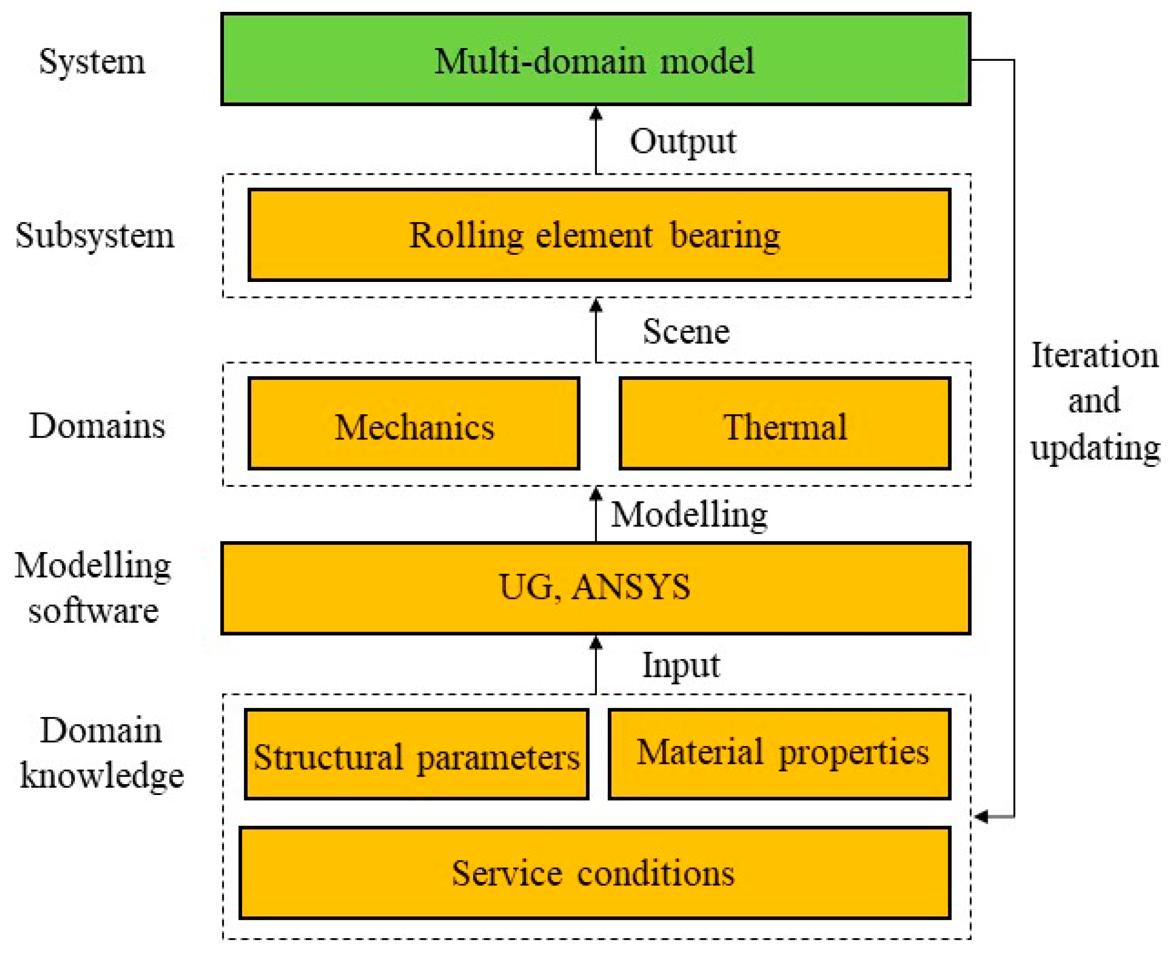
Figure 3 shows the DT model implementation. During DT model building, multi-domain knowledge (e.g., structural parameters, material properties, and service conditions) must be considered simultaneously. Multi-domain modeling software contains ANSYS and UG. Therefore, object models from the REB system can be constructed and embedded into a unified multi-domain model.

(1)

REB heat calculation

The heat of REB is generated by internal friction. The friction torque plays a decisive role in the heat generation of REB. The heat calculation is the foundation of the REB thermal analysis. Based on the measurement results of the REB friction torque, we divide the REB friction torque into the load friction torque and the viscous friction torque. The calculation formulas for the load friction torque and the viscous friction torque are given by [32]:

$$\begin{array}{c}{M}_f=M_l+M_v\\ M_l=f_1{P}_1{D}_m\\ M_v=\left\{\begin{array}{c}{10}^3{f}_0{\left(vn\right)}^{\frac{2}{3}}{D}_m^3\\ 16f_0{D}_m^3\end{array}\right.\end{array}$$

(7)

where $M_f$ represents the total friction torque; $M_l$ represents the friction torque related to a load; $M_v$ represents the friction torque related to lubricating oil properties; n represents the REB speed; v represents the kinematic viscosity of the lubricating oil; $f_0$ and $f_1$ are the correlation coefficient; $P_1$ represents the calculated load. The heat generation of REB can be expressed as the product of the friction torque and the REB angular velocity [32]:

$$H_{bear}=\frac{\pi n{M}_f}{30}$$

(8)

Convective heat transfer is the most important heat transfer method of REB. It is also the most difficult form of heat transfer to quantitatively calculate. When the low-temperature lubricating oil flows through the inner and outer raceway surfaces, rolling element (RB) surfaces, and cage surfaces of the high-temperature REB, the heat generated by REB friction is transferred to the lubricating oil through the convective heat transfer. Then, the lubricating oil transfers the heat to other components of REB. The convective heat transfer coefficient is given by [32]:

$$\alpha =0.332\frac{k}{D_m}{P}_r^{\frac{1}{3}}{R}_e^{\frac{1}{2}}$$

(9)

where $k$ is the thermal conductivity; $P_r$ is the Ludwig Prandtl number; $R_e$ represents the Reynolds number, $R_e=vx/v_0$; $v_0$ is the kinematic viscosity. When the REB transfers heat to the lubricating oil, $x=D_m$, v represents the surface velocity of the cage; when the inner wall of the REB cavity transfers heat to the lubricating oil, $x=D_h$, $v$ is taken as 1/3 of the cage surface velocity.

The heat transfer coefficient between the REB surface and the air is given by [32]:

$$\begin{array}{c}\alpha =\left\{\begin{array}{c}0.3\left(T-T_a\right),\begin{array}{cc}& \mathrm{Natural} \mathrm{convection}\end{array}\\ 0.3\frac{k_a}{D_h}{R}_e^{0.57},\begin{array}{cc}& \mathrm{Forced} \mathrm{convection}\end{array}\end{array}\right.\\ R_e=\frac{v{D}_h}{v_a}\end{array}$$

(10)

where $T_a$ is the ambient temperature around the casing; $D_h$ is the diameter of the casing; $k_a$ is the thermal conductivity of air; $v$ is the airflow velocity; $v_a$ is the kinematic viscosity of air.

After calculating the REB heat generation and the convective heat transfer coefficient, the steady-state thermal analysis module of ANSYS Workbench performs the thermal analysis of REB. First, we set the basic properties of REB, and then we divide the mesh. Due to the mesh division’s impact on the solution accuracy, we refine the mesh of the contact area. Finally, the boundary condition setting is analyzed by two types of constraints. One is the loading heat flux on the surface of the RBs in contact with the raceway. The other is the load thermal convection on the surface of the inner and outer rings and the RBs.

(2)

REB load distribution

The centrifugal force and the gyroscopic moment generated by the RB are small. The influence of these factors can be ignored when we calculate and analyze the load distribution. The RB load can be analyzed statically, and the contact angle between the RB and the inner and outer rings is assumed to be equal. When the REB only bears the radial load $F_r$, the upper half RBs of the REB are not loaded. However, the lower half RB of the REB is loaded. Figure 4 shows the load distribution of REB. Under the action of the radial load $F_r$. The inner and outer rings move radially by a distance of ${\delta }_r$. The RB located on the external force line is the most loaded, and the maximum contact deformation is given by [32]:

$${\delta }_{\max }={\delta }_r-\frac{G_r}{2}$$

(11)

where ${\delta }_{\max }$ represents the elastic deformation at the RB maximum load; ${\delta }_r$ represents the radial deformation; $G_r$ represents the working clearance.

According to the deformation coordination conditions, the deformation amount at the contact between each RB and the raceway is given by [32]:

$${\delta }_{\mathrm{\Psi }}={\delta }_r\cos \mathrm{\Psi }-\frac{G_r}{2}={\delta }_{\max }\left(1-\frac{1-\cos \mathrm{\Psi }}{\frac{2{\delta }_{\max }}{2{\delta }_{\max }+G_r}}\right)$$

(12)

where $\mathrm{\Psi }$ represents the angle between the center of each RB and the maximum load of RB; ${\delta }_{\mathrm{\Psi }}$ is the elastic deformation at the RB maximum load. $\epsilon$ is given by [32]:

$$\epsilon =\frac{1}{2}\left(1-\frac{G_r}{2{\delta }_{\max }+G_r}\right)$$

(13)

where $\epsilon$ represents the load distribution parameter of REB. It is the size of the load zone range of REB.

According to the Hertz contact theory, the RB load at any position is given by [32]:

$$Q_{\mathrm{\Psi }}=Q_{\max }{\left[1-\frac{1}{2\epsilon }\left(1-\cos \mathrm{\Psi }\right)\right]}^t$$

(14)

(3)

RUL mathematical model of REB

The REB fatigue life is given by [32]:

$$L10={(C/P)}^p$$

(15)

where $L10$ represents that the REB can meet the predetermined load within 90% of its service life; $C$ represents the basic dynamic load capacity; $P$ represents the actual load; $p$ represents the Exponent constant.

The remaining useful life of rolling element bearing is given by [32]:

$$RUL=\left(L10-L\right)/L10 \times 100\%$$

(16)

where RUL represents the percentage of remaining useful life; L10 represents the fatigue life of REB; L represents the actual service life. By Equation (16), the remaining useful life of rolling element bearing can be estimated. We can plan the replacement of REB and avoid the losses caused by the REB failure.

The Implementation of the LSTM Model

Figure 5 shows the specific implementation process of the RUL prediction model based on LSTM. The inputs of the RUL model are the REB full life cycle signal data. First, it is necessary to preprocess the data. Then, the preprocessed data is separated into the training group and the test group. Next, we normalize the feature data. Finally, an LSTM network is constructed and trained to obtain the predicted RUL value.

The Implementation of the Hybrid Method

Using the fusion method, the predicted RUL of LSTM is taken as the systematic observation value to correct the theoretical and empirical derivation results driven by the DT model. PSO used in this paper is a fusion algorithm. The steps of the hybrid method are shown in Figure 6.

(1)

Establish an LSTM model for the REB system and use the predicted RUL value obtained from the model as an observation value.

(2)

According to the RUL variation rules of the DT model, it is converted into an RUL space model for initialization based on the PSO algorithm, and the internal state of the system is calculated using model simulation.

(3)

Initialize the PSO algorithm based on the RUL space model and use the observed values to modify the theoretical values obtained from the system model simulation and reasoning. We can obtain more accurate RUL prediction values.

(4)

Judge whether the predicted value of the RUL reaches the threshold value based on the analysis results of the PSO algorithm. If the predicted value of the RUL reaches the threshold value, we should make appropriate maintenance. Otherwise, return to (2) to repeat the iteration.

Take PSO for example, the state equation of the system is given by [33].

$$x_k=f_k\left(x_{k-1},v_{k-1}\right)$$

(17)

where $x$ represents the system state, $f$ represents the system state transition function, and $v$ represents the system noise. The measurement equation of the system is shown as Equation (18), in which $y$ represents the measured system state, $h$ represents the measurement function, and $n$ represents the measurement noise.

$$y_k=h_k\left(x_k,n_k\right)$$

(18)

PSO includes two processes: prediction and updating. In the prediction process, Bayesian calculation as used in Equations (19)–(21) is used to estimate the next state according to the prior probability density of the system, and the updating process uses the measured data to modify the prediction results.

$$p\left(x_k\left|x_k\right.\right)=\frac{p\left(y_{1:k}\left|x_k\right.\right)p\left(x_k\left|y_{1:k-1}\right.\right)}{p\left(y_{1:k}\right)}$$

(19)

$$\begin{array}{c}p\left(x_k\left|y_{1:k-1}\right.\right)={\displaystyle \int p\left(x_k,x_{k-1}\left|y_{1:k-1}\right.\right)}d{x}_{k-1}\\ p\left(x_k\left|y_{1:k-1}\right.\right)={\displaystyle \int p\left(x_k,x_{k-1}\right)p\left(x_{k-1}\left|y_{1:k-1}\right.\right)}d{x}_{k-1}\end{array}$$

(20)

$$p\left(y_{1:k}\right)={\displaystyle \int p\left({\mathrm{y}}_k{\left|x\right.}_k\right)p\left(x_k\left|y_{1:k-1}\right.\right)}d{x}_k$$

(21)

The integration of Equation (21) in Bayesian calculation is replaced by Monte Carlo sampling as Equation (22) and the average value of the sampled particles is calculated to get the expected value.

$$E\left[f\left(x_n\right)\right]\approx \frac{1}{N}{\displaystyle \sum _{i=1}^{N}f\left(x_n^{\left(i\right)}\right)}$$

(22)

PSO refers to the process of approximating the probability density function by finding a set of random samples propagating in the state space and replacing the integral operation with the sample mean to obtain the minimum variance distribution of the state. When the number of particles $N\to \infty$, it can approach any form of probability density distribution. Therefore, the prediction result is more accurate than the theoretical derivation and observation value.

The Hybrid Method in the PHM System

As an indispensable key component in industrial machinery and equipment, REBs are related to the safety and stability of the equipment. As an important technology of rolling element bearing prediction and health management, the RUL prediction can effectively estimate their remaining life, so as to realize early intervention and maintenance of mechanical equipment and ensure the safety of enterprises’ production [34]. In this paper, REB is diagnosed, predicted, and optimized using the hybrid method separately and it is assigned different weights to make up the whole predictive maintenance.

4. Case Study

4.1. Experiment Platform and Database

Figure 7 shows the testing platform for the REB accelerated life test. These data are collected from one REB vibration signal at a speed of 2100 r/min and a radial load of 12 kN. We set the sampling frequency at 25.6 kHz, the sampling duration at 1.28 s, and the sampling interval at 1 min. Under this working condition, the total lifespan of REB is around 2 h and 30 min. The REB has an outer ring fault. One temperature sensor is arranged on the REB system to measure the temperature changes. One strain gauge load sensor is applied to measure the load changes. One vertical accelerometer and one horizontal accelerometer are installed on the REB system to measure the vibration signal. We divide the dataset of the full life cycle vibration signals of the bearing. A total of 70% of the bearing data is divided into a training set by proportional sampling, and 30% of the bearing data is divided into a testing set to test the LSTM model. The data information used in the experiment is shown in

Table 1. Summary of experiment data.

	Total Dataset	Trainset	Testset
Rolling Element Bearing	12,200	8540	3660

.

4.2. DT-Based Hybrid RUL Prediction Approach for REB

4.2.1. The Realization of the DT Model

To construct a DT model,

Table 2. The material parameters of REB.

Part	REB
Material	GCr15
Density/(g/m2)	7.83
Modulus of elasticity E/GPa	2.19
Poisson’s ratio μ	0.3
Thermal conductivity/(W/m°C)	49
Coefficient of thermal expansion/(°C−1)	13.5 × 10−6

and

Table 3. The structure parameters of REB.

Number	Parameter Name	Value
1	Inner diameter	30 mm
2	Outer diameter	62 mm
3	Pitch diameter	46 mm
4	Ball diameter	9.25 mm
5	REB width	16 mm
6	Number of balls	8
7	Coefficient of curvature radius of inner groove	0.515
8	Coefficient of curvature radius of external groove	0.52

show the material and structure parameters of REB, respectively.

To facilitate the DT model establishment of REB, we use UG software to appropriately simplify the three-dimensional model of REB. The simplified model is imported into Workbench software. Then, in order to simplify the calculation process, a two-dimensional axisymmetric model is drawn based on the cross-sectional dimensions. Finally, to ensure the convergence of the entire model and the accuracy of the temperature distribution results, the grid division of the heat transfer concentration area near the REB is relatively dense, and the grid division of the inner cavity and outer surface edge areas of REB is relatively sparse. After adding the temperature measuring point and the load measuring point, the DT system starts to measure the REB temperature and correct the thermal boundary. The temperature field of REB is shown in Figure 8. Rolling element bearing contains RBs, an inner ring, an outer ring, and a cage. The overall introduction structure is too complex, which affects the calculation speed and makes the calculation results inaccurate. Considering the symmetry characteristics of REB, we use a single RB and a combination of inner and outer rings as the analysis unit. The entire structure analysis can be achieved by the cyclic symmetry constraints. The RB thermal stress nephogram is shown in Figure 9.

Figure 10 shows the comparison between the simulated vibration signal and the actual vibration signal of REB. Figure 11 shows a comparison between the simulated REB load and the actual REB load. The experimental results show that the simulated vibration signal accuracy of DT is above 97.8%, and the simulated load distribution accuracy is up to 96.5%. This proves that the proposed DT model can reflect the actual thermal characteristics.

4.2.2. The Realization of the LSTM Model

First, we smoothed the collected data. Taking the horizontal vibration signal as an example, Figure 12 is the collected vibration signal data. The curve has a lot of noise. Therefore, it needs to be smoothed. To reduce the computational complexity, we adopted the moving average filtering method. The smoothing result is shown in Figure 13. After noise elimination, we chose 70% for the training group and 30% for the test group. The normalization formula is given by [35]:

$${\mathrm{x}}_{\mathrm{i}}^{\prime }=\frac{{\mathrm{x}}_{\mathrm{i}}-{\mathrm{x}}_{\min }}{{\mathrm{x}}_{\max }-{\mathrm{x}}_{\min }}$$

(23)

This paper builds an LSTM neural network based on the Python framework. Due to the complexity and depth of the model structure, it is necessary to simplify the model structure. To select a suitable model structure, we conducted the relevant experiments. As shown in

Table 4. The maximum residual error corresponding to different LSTM layers and hidden node numbers.

Model Structure	LSTM Two-Layer Maximum Residual Error (μm)	LSTM Three-Layer Maximum Residual Error (μm)	LSTM Four-Layer Maximum Residual Error (μm)
eight hidden nodes	11.6	8	17
twelve hidden nodes	7	10.4	20
sixteen hidden nodes	9	12.6	25.3
twenty hidden nodes	10.3	11	17.6

, we can obtain the maximum residual value of the RUL prediction by setting different LSTM layers and hidden node numbers. The maximum residual error of the LSTM with two layers and twelve hidden nodes is the smallest, which has the highest accuracy.

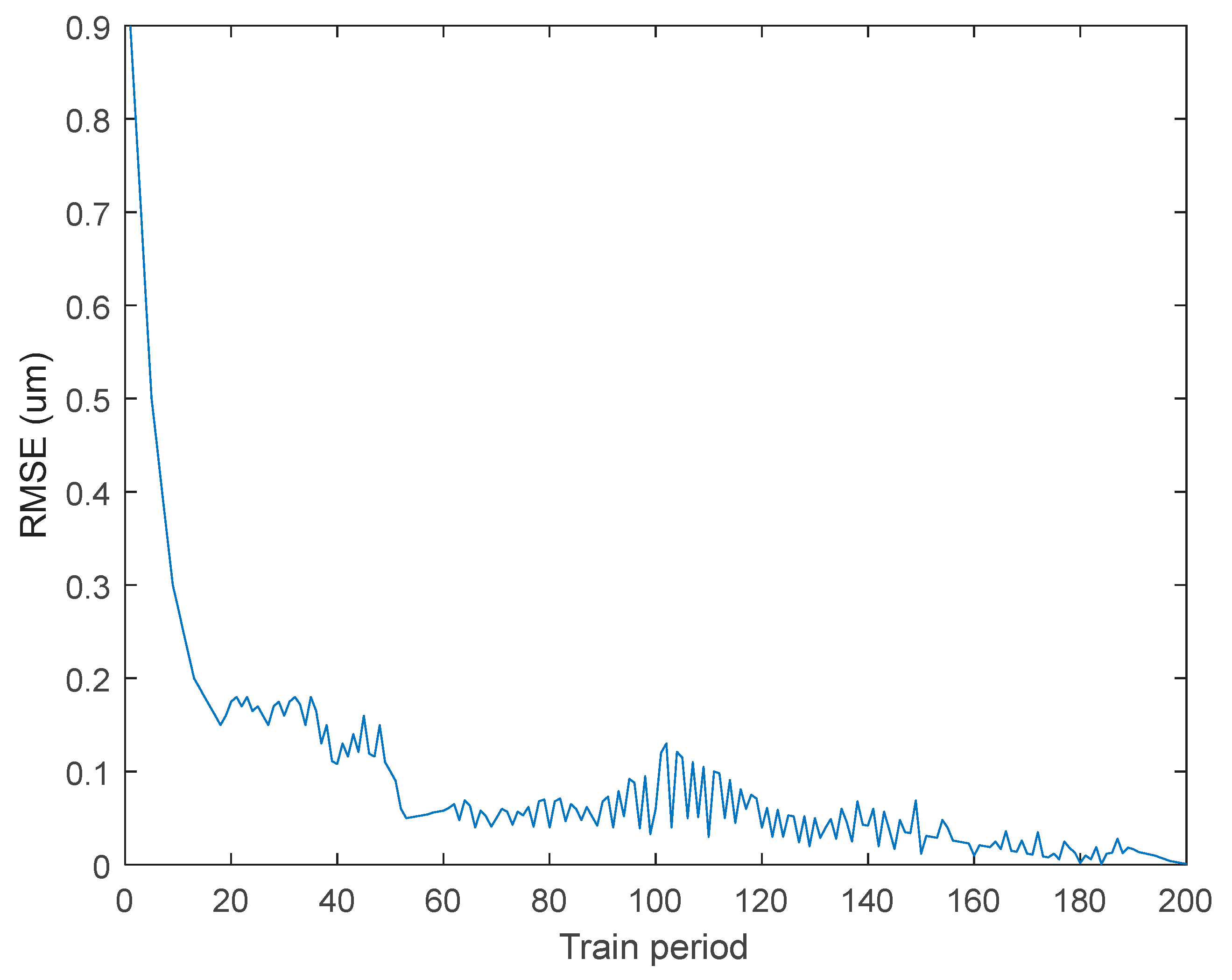
After repeated experiments, we chose the LSTM structure with four layers, which include one input layer, two hidden layers, one output layer, six input layer nodes, twelve hidden layer nodes, and two output layer nodes. We used the gradient descent method to find the optimal solution, and the training results display the maximum residuals of the predicted value. We set the number of iterations as 1000 and the learning rate as 0.1. The model parameters are randomly initialized. The root mean square error (RMSE) convergence curve during training is shown in Figure 14.

4.2.3. The Realization of the Hybrid Method

In this research, theoretical values with DT and LSTM-driven RUL predicted values are fused in the PSO algorithm. The RUL prediction from the LSTM-driven method is taken as the observation value of the PSO algorithm to adjust the theoretical value of RUL. Equation (16) shows the RUL theoretical value of REB, which is used as the system state equation of PSO to initialize the algorithm. Meanwhile, the actual value of the RUL obtained by LSTM is shown in Equation (6), which is used as the system observation value of PSO. The number of particles is set to 150. The Algorithm 1 is shown below.

Algorithm 1: The Hybrid Method for the RUL Prediction of REB

Input: The theoretical prediction value of DT and the actual prediction value of LSTM Output: The particles prediction value (1) Initialize the parameters and particles (2) $RUL=\left(L10-L\right)/L10 \times 100\%$ (3) $h_t=o_t\cdot \tanh \left(C_t\right)$ for 1 = 1:150 (4) Sample from (2) (5) Calculate the RUL prediction value ${\mathrm{h}}_{ti}$ of particles by (3) (6) Calculate the weight $RUL(i)$ of each particle end (7) Normalize the weight (8) Resample according to the normalized weight (9) Output the RUL prediction value $h_f$ of REB

The $h_f$ value is the final RUL predicted by the hybrid approach. REB maintenance is conducted if $h_f$ has reached the threshold; otherwise, the RUL is predicted by the hybrid approach again [33].

Table 5. The robustness evaluation of different methods.

Method	Robustness
DT	0.754
LSTM	0.841
Hybrid Method	0.96

shows the robustness evaluation of different methods. Therefore, compared with DT and LSTM, the hybrid method has strong robustness. The robustness is given by [36].

$$\mathrm{Rob}\left(\mathrm{X}\right)=\frac{1}{n}{\displaystyle \sum }_{i=1}^n\left(-\left|\frac{x_i-\tilde{x}}{x_i}\right|\right)$$

(24)

where $x_i$ represents the remaining useful life value of remaining useful life. $\tilde{x}$ represents the mean value of $x_i$.

4.3. The Analysis of Experimental Results

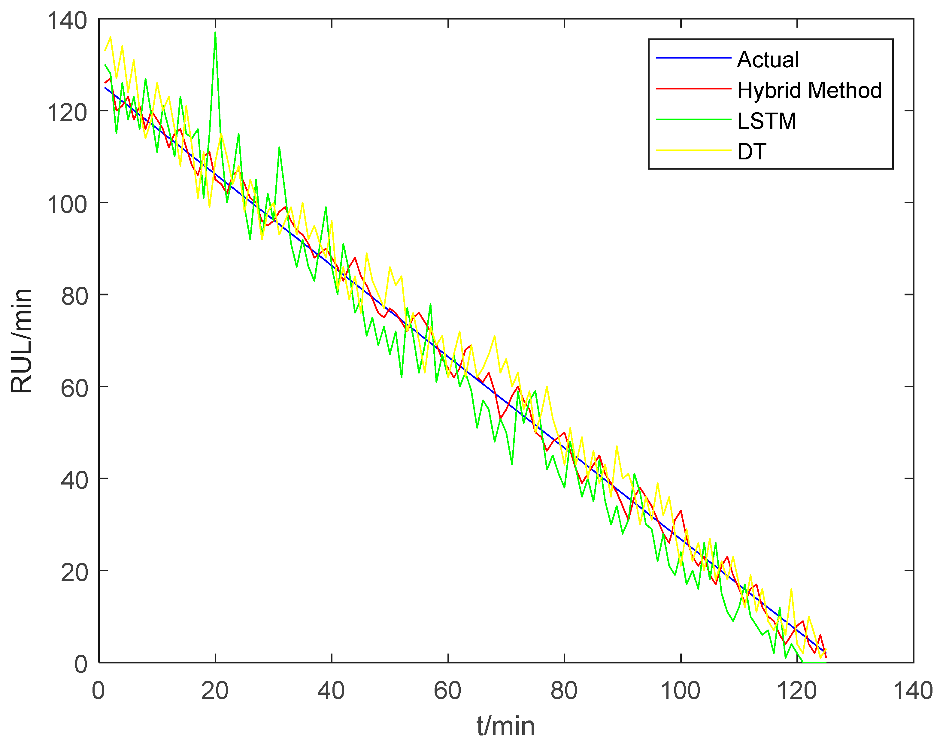
The RUL prediction result of REB is shown in Figure 15. Well-known hybrid algorithms are Karman Filter, PSO, and Ensemble Learning. We compared the three hybrid algorithms in Figure 16. It indicated that the PSO algorithm has the best prediction performance. When we use single prediction methods (e.g., DT and LSTM), there is a significant error between the predicted value and the actual value. When we use a hybrid method based on DT, the predicted value is closer to the actual value, and the prediction accuracy is improved. The hybrid method overcomes the model inconsistency of DT and the poor adaptability of LSTM. The prediction accuracy of the hybrid method is greater than 97.5%, which improves the prediction accuracy and robustness of RUL.

Figure 15 shows the RUL prediction value of different methods. When we use single prediction methods (e.g., DT and LSTM), there is a significant error between the predicted value curve and the actual curve. When we use the hybrid method, the predicted curve is close to the actual curve, and the prediction accuracy is improved. The hybrid method overcomes the model inconsistency of DT and the poor adaptability of LSTM. The hybrid method has a higher accuracy than the single method by nearly 11.5%, which improves the prediction performance and robustness of RUL.

Table 6. The quantitative evaluation of different methods.

Method	Start Stage Accuracy	Middle Stage Accuracy	End Stage Accuracy	Average Accuracy
DT	90%	87%	81%	86%
LSTM	97.5%	89.5%	84.5%	90.5%
Hybrid Method	100%	97.5%	95%	97.5%

shows the quantitative evaluation of different methods.

Table 7. The accuracy comparison of different methods.

Method	Accuracy
MMA-BiLSTM [23]	90.33%
Co-Simulation-Based DT [37]	92.39%
Linear Mapping Method [38]	96.86%
Hybrid Method	97.5%

shows the accuracy comparison of different methods. The result indicates that the hybrid method has higher accuracy at all stages compared with DT and LSTM. The average accuracy of LSTM is 97.5%. Meanwhile, the hybrid method shows better prediction performance compared with the other method.

5. Conclusions

To enhance the RUL prediction accuracy of REB, we propose a novel RUL prediction method based on DT. Firstly, we established a DT system to simulate the thermal characteristics and the load distribution of REB. Based on the simulated result, we can obtain the theoretical value of RUL. Then, LSTM was constructed to analyze the experimental data. The output of LSTM is the actual value of RUL. Finally, we used the PSO algorithm to fuse the theoretical values of DT with the actual values of LSTM. The hybrid method was compared with the single method, and the accuracy of the hybrid method was greater than 97.5%. Therefore, the hybrid method can predict the remaining useful life of rolling element bearing effectively and provide a theoretical basis for the RUL warning of REB. This paper only verifies the method for REB. In the future, the hybrid method will be applied to the other components. Real time is a crucial aspect of RUL prediction. The simulation of the DT physical performance model consumes much computing resources and time. In the future, we will improve the real-time performance and computational efficiency of DT simulation.

References

- Deng, F.; Chen, Z.; Liu, Y.; Yang, S.; Hao, R.; Lyu, L. A novel combination neural network based on ConvLSTM-Transformer for bearing remaining useful life prediction. Machines 2022, 10, 1226. [Google Scholar] [CrossRef]
- Li, X.; An, S.; Shi, Y.; Huang, Y. Remaining useful life estimation of rolling bearing based on SOA-SVM algorithm. Machines 2022, 10, 729. [Google Scholar] [CrossRef]
- Lei, Y.; Li, N.; Guo, L.; Li, N.; Yan, T.; Lin, J. Machinery health prognostics: A systematic review from data acquisition to RUL prediction. Mech. Syst. Signal Process. 2018, 104, 799–834. [Google Scholar] [CrossRef]
- Zimmermann, N.; Lang, S.; Blaser, P.; Mayr, J. Adaptive input selection for RUL compensation models. CIRP Ann. 2020, 69, 485–488. [Google Scholar] [CrossRef]
- Liang, Y.C.; Li, W.D.; Lou, P.; Hu, J.M. RUL prediction for heavy-duty CNC machines enabled by long short-term memory networks and fog-cloud architecture. J. Manuf. Syst. 2022, 62, 950–963. [Google Scholar] [CrossRef]
- Srikanth, I.; Arockiasamy, M. Deterioration models for prediction of remaining useful life of timber and concrete bridges: A review. J. Traffic Transp. Eng. 2020, 7, 152–173. [Google Scholar] [CrossRef]
- Yan, M.; Wang, X.; Wang, B.; Chang, M.; Muhammad, I. Bearing remaining useful life prediction using support vector machine and hybrid degradation tracking model. ISA Trans. 2020, 98, 471–482. [Google Scholar] [CrossRef]
- Li, X.; Cheng, J.; Shao, H.; Liu, K.; Cai, B. A fusion CWSMM-based framework for rotating machinery fault diagnosis under strong interference and imbalanced case. IEEE T. Ind. Inform. 2021, 18, 5180–5189. [Google Scholar] [CrossRef]
- Yan, X.; She, D.; Xu, Y.; Jia, M. Deep regularized variational autoencoder for intelligent fault diagnosis of rotor-bearing system within entire life-cycle process. Knowl.-Based Syst. 2021, 226, 107142. [Google Scholar] [CrossRef]
- Li, Y.; Huang, X.; Ding, P.; Zhao, C. Wiener-based remaining useful life prediction of rolling bearings using improved Kalman filtering and adaptive modification. Measurement 2021, 182, 109706. [Google Scholar] [CrossRef]
- Tao, F.; Zhang, H.; Liu, A.; Nee, A.Y. Digital twin in industry: State-of-the-art. IEEE T. Ind. Inform. 2018, 15, 2405–2415. [Google Scholar] [CrossRef]
- Ma, M.; Mao, Z. Deep-convolution-based LSTM network for remaining useful life prediction. IEEE Trans. Ind. Inform. 2020, 17, 1658–1667. [Google Scholar] [CrossRef]
- Shi, Z.; Chehade, A. A dual-LSTM framework combining change point detection and remaining useful life prediction. Reliab. Eng. Syst. Saf. 2021, 205, 107257. [Google Scholar] [CrossRef]
- Park, K.; Choi, Y.; Choi, W.J.; Ryu, H.Y.; Kim, H. LSTM-based battery remaining useful life prediction with multi-channel charging profiles. IEEE Access 2020, 8, 20786–20798. [Google Scholar] [CrossRef]
- Ren, L.; Dong, J.; Wang, X.; Meng, Z.; Zhao, L.; Deen, M.J. A data-driven auto-CNN-LSTM prediction model for lithium-ion battery remaining useful life. IEEE Trans. Ind. Inform. 2020, 17, 3478–3487. [Google Scholar] [CrossRef]
- Liu, J.; Lei, F.; Pan, C.; Hu, D.; Zuo, H. Prediction of remaining useful life of multi-stage aero-engine based on clustering and LSTM fusion. Reliab. Eng. Syst. Saf. 2021, 214, 107807. [Google Scholar] [CrossRef]
- Zhao, C.; Huang, X.; Li, Y.; Li, S. A novel cap-LSTM model for remaining useful life prediction. IEEE Sens. J. 2021, 21, 23498–23509. [Google Scholar] [CrossRef]
- Liu, C.; Zhang, Y.; Sun, J.; Cui, Z.; Wang, K. Stacked bidirectional LSTM RNN to evaluate the remaining useful life of supercapacitor. Int. J. Energy Res. 2022, 46, 3034–3043. [Google Scholar] [CrossRef]
- Fu, S.; Zhang, Y.; Lin, L.; Zhao, M.; Zhong, S.S. Deep residual LSTM with domain-invariance for remaining useful life prediction across domains. Reliab. Eng. Syst. Saf. 2021, 216, 108012. [Google Scholar] [CrossRef]
- Guo, J.; Yang, Z.; Chen, C.; Luo, W.; Hu, W. Real-time prediction of remaining useful life and preventive maintenance strategy based on digital twin. J. Comput. Inf. Sci. Eng. 2021, 21, 031003–031017. [Google Scholar] [CrossRef]
- He, B.; Liu, L.; Zhang, D. Digital twin-driven remaining useful life prediction for gear performance degradation: A review. J. Comput. Inf. Sci. Eng. 2021, 21, 030801. [Google Scholar] [CrossRef]
- Meraghni, S.; Terrissa, L.S.; Yue, M.; Ma, J.; Jemei, S.; Zerhouni, N. A data-driven digital-twin prognostics method for proton exchange membrane fuel cell remaining useful life prediction. Int. J. Hydrog. Energy 2021, 46, 2555–2564. [Google Scholar] [CrossRef]
- Zhang, R.; Zeng, Z.; Li, Y.; Liu, J.; Wang, Z. Research on Remaining Useful Life Prediction Method of Rolling Bearing Based on Digital Twin. Entropy 2022, 24, 1578. [Google Scholar] [CrossRef] [PubMed]
- Moghadam, F.K.; Nejad, A.R. Online condition monitoring of floating wind turbines drivetrain by means of digital twin. Mech. Syst. Signal Process. 2022, 162, 108087. [Google Scholar] [CrossRef]
- Qu, X.; Song, Y.; Liu, D.; Cui, X.; Peng, Y. Lithium-ion battery performance degradation evaluation in dynamic operating conditions based on a digital twin model. Microelectron. Reliab. 2020, 114, 113857. [Google Scholar] [CrossRef]
- Xiong, M.; Wang, H.; Fu, Q.; Xu, Y. Digital twin-driven aero-engine intelligent predictive maintenance. Int. J. Adv. Manuf. Technol. 2021, 114, 3751–3761. [Google Scholar] [CrossRef]
- Aivaliotis, P.; Georgoulias, K.; Chryssolouris, G. The use of Digital Twin for predictive maintenance in manufacturing. Int. J. Comput. Integr. Manuf. 2019, 32, 1067–1080. [Google Scholar] [CrossRef]
- Liu, R.J.; Li, H.S.; Lv, Z.H. Modeling methods of 3D model in digital twins. CMES-Comp. Model. Eng. 2023, 136, 985–1022. [Google Scholar] [CrossRef]
- Grieves, M.W. Product lifecycle management: The new paradigm for enterprises. Int. J. Prod. Dev. 2005, 2, 71–84. [Google Scholar] [CrossRef]
- Smagulova, K.; James, A.P. A survey on LSTM memristive neural network architectures and applications. Eur. Phys. J. Spec. Top. 2019, 228, 2313–2324. [Google Scholar] [CrossRef]
- Korstanje, J. LSTM RNNs. In Advanced Forecasting with Python: With State-of-the-Art-Models Including LSTMs, Facebook’s Prophet, and Amazon’s DeepAR; Apress: Berkeley, CA, USA, 2021; pp. 243–251. [Google Scholar]
- Chen, Z.C.; Chen, Z.N. Termal Characteristics Foundation of Machine Tools; Machinery Industry Press: Beijing, China, 1989. [Google Scholar]
- Marini, F.; Walczak, B. Particle swarm optimization (PSO). A tutorial. Chemom. Intell. Lab. Syst. 2015, 149, 153–165. [Google Scholar] [CrossRef]
- Vrignat, P.; Kratz, F.; Avila, M. Sustainable manufacturing, maintenance policies, prognostics and health management: A literature review. Reliab. Eng. Syst. Saf. 2022, 218, 108140. [Google Scholar] [CrossRef]
- Tang, X.; Liu, K.; Lu, J.; Liu, B.; Wang, X.; Gao, F. Battery incremental capacity curve extraction by a two-dimensional Luenberger-Gaussian-moving-average filter. Appl. Energy 2020, 280, 115895. [Google Scholar] [CrossRef]
- Baker, J.W.; Schubert, M.; Faber, M.H. On the assessment of robustness. Struct. Saf. 2008, 30, 253–267. [Google Scholar] [CrossRef]
- Xia, M.; Li, T.; Shu, T.; Wan, J.; De Silva, C.W.; Wang, Z. A two-stage approach for the remaining useful life prediction of bearings using deep neural networks. IEEE Trans. Ind. Inform. 2018, 15, 3703–3711. [Google Scholar] [CrossRef]
- Wang, Q.; Xu, K.; Kong, X.; Huai, T. A linear mapping method for predicting accurately the RUL of rolling bearing. Measurement 2021, 176, 109127. [Google Scholar] [CrossRef]
Figure 1.
The framework of LSTM.
Figure 2.
The framework of the hybrid method.
Figure 3.
The implementation of DT model.
Figure 4.
The load distribution of REB.
Figure 5.
The implementation process of the LSTM model.
Figure 6.
The steps of the hybrid method.
Figure 7.
The structure of the REB system.
Figure 8.
The temperature field of REB.
Figure 9.
The ball thermal stress nephogram of RB.
Figure 10.
The vibration signal of REB.
Figure 11.
The rolling element load distribution of REB.
Figure 12.
The collected vibration signal data.
Figure 13.
The collected vibration signal after smoothing.
Figure 14.
The RMSE convergence curve of LSTM.
Figure 15.
The RUL prediction value of different methods.
Figure 16.
The comparison of different hybrid algorithms.