


Repeated Collision of a Planar Robotic Arm with a Surface Using Generalized Active Forces


1
Mechanical Engineering Department, Auburn University, Auburn, AL 36849, USA
2
Faculty of Mechanics, University of Craiova, 200585 Craiova, Romania
*
Author to whom correspondence should be addressed.
Machines 2023, 11(8), 773; https://doi.org/10.3390/machines11080773
Submission received: 13 June 2023
/
Revised: 18 July 2023
/
Accepted: 21 July 2023
/
Published: 25 July 2023
(This article belongs to the Special Issue Motion Optimization of Mechanical Structures)
Abstract
:The periodic impact of a planar two-arm robot is investigated in this study. Lagrange’s equations of motion are developed, and the symbolic expression of the generalized active forces are used for the control torques. The actuator torques derived with generalized active forces are compared with PD and PID controllers. The robot collides with a rebound on a rough surface. Different nonlinear functions describe the three stages of the impact: elastic compression, elasto-plastic compression, and elastic restitution. A Coulomb model describes the friction force and the sliding velocity at the impact point. At the end of the impact period, the kinetic energy of the non-impacting link is increasing, and the total kinetic energy of the robot decreases. The motion of the robot with generalized active forces controllers is periodic. The important implication of this study is the generalized forces controller and the impact with friction for the periodic robot.
1. Introduction
Impact refers to transferring energy from one body to another due to a collision or sudden shock. This can cause deformation to the objects involved. Stereo mechanics studies collisions with the conservation of momentum and the coefficient of restitution (CoR). Various CoR models are proposed as a measure of impact dynamics: (i) kinematic coefficient of restitution by Newton [1], (ii) kinetic coefficient of restitution by Poison [2], and (iii) energetic coefficient of restitution by Stronge [3]. The system’s dynamics is susceptible to the variation of CoR [4]. Another approach to the impact dynamics problem is numerically simulating impact using several contact mechanic models. Chatterjee et al. [5] presented a new approach to the impact problem, reformulating impulse-momentum equations by relaxing the rigidity assumptions to allow small deformations at the contact points. The authors provided numerical simulations, yet the study lacks experimental validation. Green [6] combined an elasto-plastic contact model [7] and Zenner model [8], which only focuses elastic waves instigated in an elastic impact. Green applied the method to a large range of materials and their results agreed well with the experiments. A good review of the available contact models can be found in [9].
It is hard to understand the local behavior of complex and multibody systems due to the lack of direct measurement techniques. Chen et al. [10] measured the local dynamics of the structure using the digital image correlation (DIC) method. The authors were able to measure separation and micro-slip behavior for the first mode and macro-slip for the second mode. Corral et al. discussed the nonlinear impact phenomena in multibody dynamics in detail [11]. The numerical solution of the collisions is a challenging computational problem. The friction force vector is against the sliding direction and is discontinuous. Using numerical computations, it is difficult to find zero sliding velocity. Smoothed friction functions are helpful to overcome any discontinuity issue and relax computation. Impact dynamics differential equations are numerically stiff [12]. Most of the time, there is a need to define proper error tolerances for the numerical solver.
In robotics, most of the time, collision with the environment is not desired for the applications. The trajectory of the robots is meticulously planned to avoid any contact. Lopez et al. [13] proposed a novel path-planning algorithm for planar robots. However, many multi-body dynamical systems exhibit impact while performing their tasks, including industrial manipulators [14,15,16], walking robots [17,18,19], and space robots [20]. The kinematic restitution coefficient describes the end-effector dynamic in many multibody dynamic studies. The energetic CoR is advantageous for systems with friction in multibody systems, and the energetic approach makes more physical sense. Flores [21] presented a comprehensive review of contact mechanics for dynamical systems. The author compared continuous approaches and non-smooth formulations. The author also illustrated several examples of applications.
Control of a robotic manipulator impact is a challenging and common problem in applications that require an automated system to interact with an environment. The control challenge is due, in part, to the impact effects that result in possible high stresses, rapid dissipation of energy, and fast acceleration and deceleration [22]. Two main approaches are widely accepted to cope with robot impact problems. The first approach is to add kinematic redundancy to the robot to reduce impulsive forces’ effects. The second approach is creating multiple control laws that activate for different dynamic configurations [23,24]. Hurmuzlu [25] studied the impact of the kinematic chain’s complementarity conditions at the contacting ends and critical configurations of rigid-body kinematic chains where the effect of the impulsive force transmitting a link to link vanishes in a chain. Aouaj et al. [26] proposed a procedure to predict the post-impact velocity of a robotic arm based on the idea of removing the post-impact oscillation component, and they acquired good agreement with the experiments.
Yoshida et al. studied the impact response of a PID-controlled space robot. They concluded that the system motion after impact and impulsive force could be reduced if the manipulator configuration before impact and the controller gains are adequately selected [27]. Bhasin et al. worked on an adaptive nonlinear Lyapunov-based controller for robotic contact with a stiff environment [28]. The authors limited the contact forces by substituting the feedback elements of the controller inside a hyperbolic tangent function, as presented in [29]. Cox et al. [30] proposed feedback linearization control for Inertially Actuated Jumping Robots. The proposed controller is advantageous to the PID controller as it accounts for nonlinearities and is beneficial to the sliding mode controller due to its simplicity. Papadopoulos et al. [31] surveyed robotic manipulation and capture in space. The authors presented many topics, including contact dynamics and feedback control for space robots.
Several studies focus on the dynamics of double link systems with revolute joints [32,33]. Pagilla and Yu [34] investigated the planar impact of a two-degree-of-freedom robot in up-elbow and down-below configurations. The impact of a two-link was studied with a Jackson-Green contact model [35]. Impact modeling with CoR, momentum equations, and contact mechanic models are available in the literature for multi-body systems [12]. Another approach to model impact in multi-body systems is to present impulsive forces with linear or nonlinear spring-damper models [17,36].
This study investigates the serial impact of a two-link planar robot. The equations of motion are obtained with the Lagrange method. The robot is controlled using a generalized active force. The impact of the robot consists of three phases: elastic compression, elasto-plastic compression, and elastic restitution. The impact response of multibody dynamic systems depends on the pre-impact configuration of the system [37]. The motion of the repeatedly impacting on the ground surface is analyzed. The impact dynamics of the system were assessed, including coefficient of restitution, change in kinetic energies, change of contact velocity, and contact forces. This study represents a new method for analyzing the impact of robotic systems. To our best knowledge, the controller with the generalized forces and the impact of the robots with a nonlinear force and three stages have yet to be studied.
2. Mathematical Model
2.1. Configuration of the Robotic Arm
We consider a robotic system with two degrees of freedom, as shown in Figure 1. The motion is constrained in the plane. The arm 1 () has mass, , and length, . The impacting arm is 2 () with, mass, , and length, . The centers of mass for the two arms, 1 and 2, are at and , respectively.
The generalized coordinates of the robotic system are and , where denotes the angle between the arm i with the x-axis. There are two revolute kinematic pairs at O and A. The moment of the ground on arm 1 is and the moment of arm 1 on arm 2 is . The moment of arm 2 on arm 1 is . The unit vectors of the rectangular cartesian axis are , and .
2.2. Equations of Motion
The system consists of four different dynamic configurations in sequence: control of the motion, elastic compression impact, elastoplastic compression impact, and restitution. The MATLAB symbolic toolbox defines the analytical expressions for the Lagrange equations of motion. The numerical solutions of the non-linear ordinary differential equations are calculated with the ode45 function. An event function is defined for each set of motion states to stop calculation, and the final values of the equation are provided to the following motion as initial conditions.
The arm 1 has an angular velocity of and the arm 2 has an angular velocity of The mass center has the position given by
and the mass center is defined by
The velocities of and are
The total kinetic energy of the robotic system is
where is the mass moment of inertia of arm 1 about the fixed point O and is the mass moment of inertia of arm 2 about . The forces of gravity on arms 1 and 2 are
Their application points are at and . The generalized active forces associated with the robotic motion are
During the impact, the generalized active forces are
where is the normal impact force and represents the friction force at the contact point B. The nonlinear Lagrange’s differential equations of motion are
2.3. Control Strategy
For the control moments, we improve the PD controller using generalized forces
where are proportional gains and are the derivative gains. The robot starts from an initial position, and arm 2 will repeatably impact a fixed surface. After impact, the upward controller with and is applied until m. Next, the downward controller with and is exerted. Arm 2 of the robot will impact a lower fixed surface during its motion; see Figure 2.
Next, we want to compare the tuned controller using the generalized active force with a PID controller. The PID control moments for relative generalized coordinates are
where the integrative gains are In this case, the equations of motion are integrodifferential, and auxiliary variables are introduced. Finally, we compared the PD controller constructed by equating and to the zero in Equation (10). Figure 3 compares the PID controller, generalized active force controller, and PD controller. The PD controller does not reach the final position (see Figure 3b). Our generalized active force controller (Q controller) arrives at the final position quicker than the PID controller and eliminates overshooting.
2.4. Contact Force during Impact
The spherical contact of the robotic arm is divided into three phases: elastic compression, elasto-plastic compression, and elastic restitution [38]. The elastic compression phase starts at the initial contact of the robotic arm with the surface and ends when the maximum flexible interference is reached. The elasto-plastic compression phase follows until the maximum interference, , is reached. Then the restitution phase starts, concluding at the separation between the robotic arm and the surface, leaving a residual interference, .
2.4.1. The Normal Impact Force
I. For the elastic compression phase, the Hertz theory is considered. The normal impact force is calculated with
where is the normal elastic interference:
The reduced modulus of elasticity, E, is defined as
where and are the moduli of elasticity of arm 2, and the fixed surfaces, and , are the Poisson ratio of arm 2 and the fixed surface. The reduced radius, R, is given by
where and are the radius of curvature of the end of arm 2 and the surface, respectively.
The initial position for the impact is given by and . The elastic compression phase terminates when . The critical interference, , at which the initial yielding starts is
where ; is the yield strength of the weaker material.
III. The normal elastic impact force for restitution is
The residual interference, , is given by [39]
where is the maximum interference.
The radius of curvature for restitution is
where .
2.4.2. The Friction Force
Many friction models are available in the literature. Pennestri et al. [40] presents and compares well-known friction models. To overcome the possible computational burden resulting from force discontinuity, smooth Coulomb friction has been implemented by the simulations. The smooth curve is used to replace the abrupt change in force around the zero tangential velocity . Kim et al. [41] discuss the performance of several smoothening functions, including the hyperbolic-tangent function. This study uses a hyperbolic-tangent smoothed Coulomb friction model [42] for the friction force at contact point B
where is the kinetic coefficient of friction and represents the velocity tolerance.
3. Results and Discussion
The robotic system is simulated for 15 motion cycles. Each cycle consists of a downward control, an impact on the ground wall, and an upward control. System parameters are shown in Table 1, and motion parameters are shown in Table 2. The robotic arm starts its motion from initial and . The arm collides with a surface at , Figure 2, and retreats to .
Figure 4 shows the change of the link angles with time. The angle of link 1 swings between and and the angle of link 2 swings between and . The figure illustrates a regular motion.
Figure 5 shows the phase portraits of the robotic motion. Figure 5a represents the evolution of , , and and Figure 5b shows and with respect to . Both phase portraits in Figure 5 show non-chaotic motion behavior. The motion starts from a distinct location and gradually submerges towards a limit cycle.
Figure 6 shows Poincare maps of the dynamic system. Figure 6a represents and at crossing and Figure 6b depicts the value of and at crossing. Even though the motion of the robot is simulated for 15 periods, the Poincare maps show four distinct crossing for the zero angular velocities of link 1 and link 2, respectively. The Poincare map of the motions illustrated non-chaotic motion. Figure 5 and Figure 6 show that the motion approaches a limit cycle after three impacts.
Figure 7 shows the velocities of the robotic arm’s end effector, B. Figure 7a illustrates x-axis velocity of B while Figure 7b depicts the y-axis velocity of the tip point. The velocity on the x-axis increases to at the beginning of the motion and later stays steady around and . The velocity on the y-axis swings between and . The velocities during the total time interval (the whole motion with impact) have a regular distribution.
Next, we analyze the impact dynamics with the flat solid surface. Figure 8 shows the indentation of the first impact. The impact duration is , the maximum compression is , and the residual interference is . There is a short interval for elastic compression and a nonlinear distribution for the elasto-plastic phase. The restitution is nonlinear and elastic. Due to the initial pre-impact, the configuration of the elastic contact phase is very short compared to the elasto-plastic compression and restitution phases. A zoomed-in window in Figure 8 shows the elastic compression phase in more detail.
Figure 9 shows the change of tangential velocity and normal velocity during the first impact, respectively. The initial contact speed on the tangential x-axis is and end of impact speed is observed . The tangential velocity during impact decreases in magnitude. The tangential velocity does not change the sign and has a continuous slip. The initial and final speeds on the normal y-axis are and , respectively. The kinematic coefficient of restitution of the first impact is .
Figure 10 represents the normal contact force of the impact, and the maximum contact force is . The elastic period for the Hertz contact force is very short. The elasto-plastic phase is represented by a nonlinear contact force and represents a more realistic depiction of the phase. This nonlinear force has not been used until now for robotics collisions and was experimentally verified [43]. An elastic force is used for the restitution phase until permanent deformation is obtained. The contact force is maximum at maximum compression when the normal velocity is zero. The time interval for restitution is less than the time interval for compression.
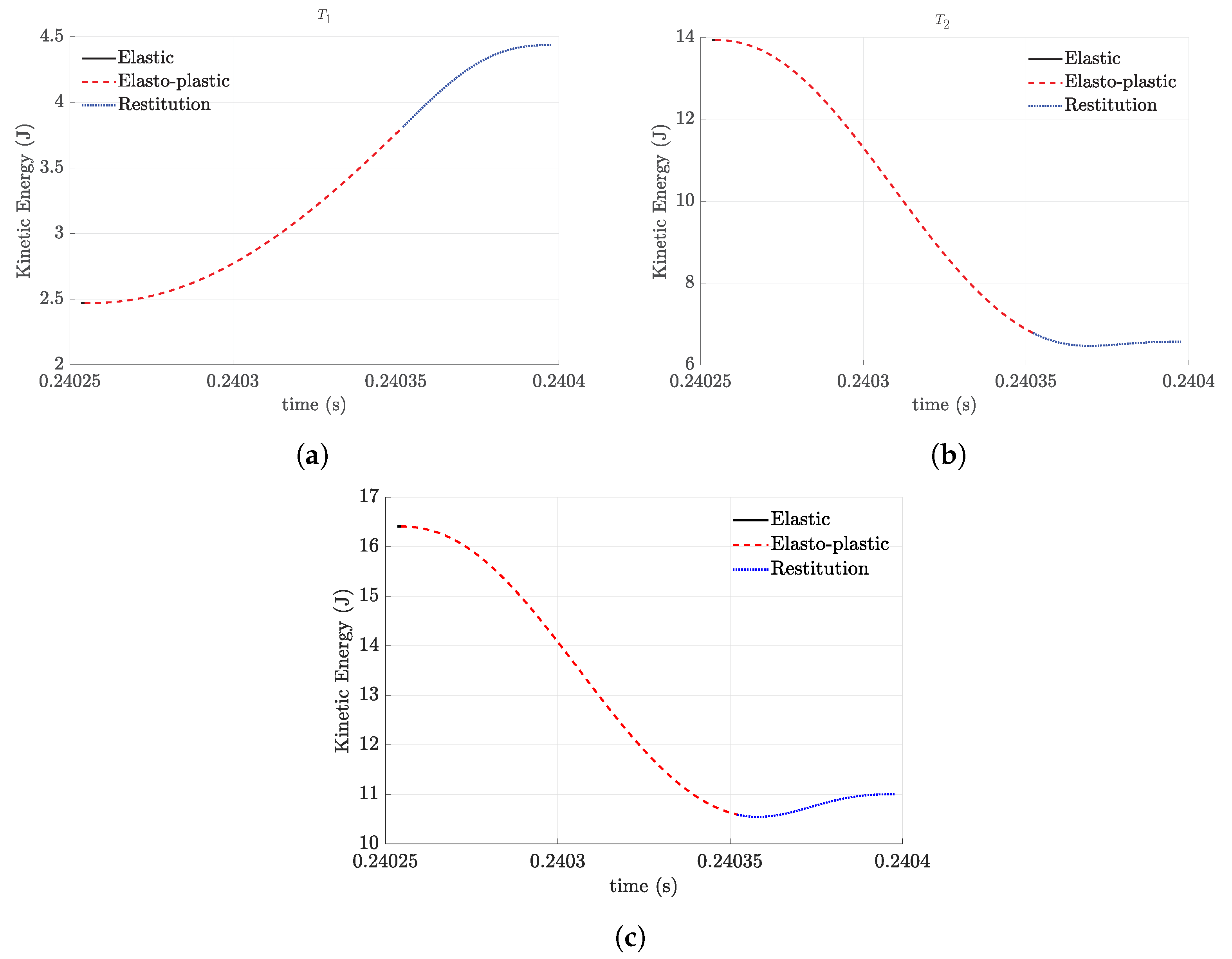
Figure 11 shows the kinetic energy change during impact. Figure 11a shows the kinetic energy of link 1. The initial kinetic energy of link 1 is and the kinetic energy after impact is . The generalized kinetic, energetic coefficient of restitution is defined as the square root of the ratio of the kinetic energy at the end of impact and the kinetic energy at the beginning of impact. The generalized energetic coefficient of the restitution [44] of link 1 is . The kinetic energy of the non-impacting arm increases during a collision. Figure 11b shows the kinetic energy of link 2. The initial kinetic energy of link 2 is and the kinetic energy after impact is . The generalized energetic coefficient of the restitution of link 2 is . Figure 11c depicts the total kinetic energy of the robotic arm. The initial kinetic energy is and the kinetic energy after impact is . The global generalized energetic coefficient of the restitution of the system is .
4. Conclusions
The periodic impact with the friction of a planar robotic arm with revolute kinematic pairs was studied using Lagrange’s equations of motion. The symbolical expressions of the generalized active forces have been employed to build control torques. The new controller was compared with the PD controller and PID controller, and its behavior was superior. The robot performed periodic operations with rebounds. The impact with friction was modeled using specific contact functions for elastic compression, elasto-plastic compression, and elastic restitution. For this new application, during the collision, the kinetic energy of the nonimpacting link increases. The total kinetic energy of the system decreases after the periodic impacts with an external surface. The motion of the kinematic chain gradually moves toward a limit cycle and shows regular behavior. The applications of research can be applied to walking machines, industrial robots, search and rescue robots hitting obstacles, and agricultural robots. For future research, the elasticity of the links should be considered, and experimental validation is needed to verify the results.
Author Contributions
Conceptualization, A.F.A. and D.B.M.; methodology, A.F.A. and D.B.M.; software, A.F.A. and D.B.M.; validation, A.F.A., D.B.M., J.Z. and Daniela Tarnita; writing—original draft preparation, A.F.A., D.B.M. and J.Z.; writing—review and editing, A.F.A., D.B.M., J.Z. and Daniela Tarnita; visualization, A.F.A., J.Z. and D.B.M.; supervision, D.B.M. All authors have read and agreed to the published version of the manuscript.
Funding
This research received no external funding.
Data Availability Statement
No data available.
Conflicts of Interest
The authors declare no conflict of interest.
References
- Newton, I. Philosophiae naturalis principia mathematica; Londini, Jussu Societatis Regiæ ac Typis Josephi Streater; Prostat apud plures Bibliopolas: Washington, DC, USA, 1687. [Google Scholar]
- Poisson, S. Mechanics; Trans. HH Harte: London, UK, 1817; Volume II. [Google Scholar]
- Stronge, W. Unraveling paradoxical theories for rigid body collisions. J. Appl. Mech. 1991, 58, 1049–1055. [Google Scholar] [CrossRef]
- Blazejczyk-Okolewska, B.; Kapitaniak, T. Dynamics of impact oscillator with dry friction. Chaos Solitons Fract. 1996, 7, 1455–1459. [Google Scholar] [CrossRef]
- Chatterjee, A.; Ghaednia, H.; Bowling, A.; Brake, M. Estimation of impact forces during multi-point collisions involving small deformations. Multibody Syst. Dyn. 2021, 51, 45–90. [Google Scholar] [CrossRef]
- Green, I. The prediction of the coefficient of restitution between impacting spheres and finite thickness plates undergoing elastoplastic deformations and wave propagation. Nonlinear Dyn. 2022, 109, 2443–2458. [Google Scholar] [CrossRef]
- Jackson, R.L.; Green, I. A finite element study of elasto-plastic hemispherical contact against a rigid flat. J. Trib. 2005, 127, 343–354. [Google Scholar] [CrossRef] [Green Version]
- Zener, C. The intrinsic inelasticity of large plates. Phys. Rev. 1941, 59, 669. [Google Scholar] [CrossRef]
- Ghaednia, H.; Wang, X.; Saha, S.; Xu, Y.; Sharma, A.; Jackson, R.L. A review of elastic–plastic contact mechanics. Appl. Mech. Rev. 2017, 69, 060804. [Google Scholar] [CrossRef] [Green Version]
- Chen, W.; Jin, M.; Lawal, I.; Brake, M.R.; Song, H. Measurement of slip and separation in jointed structures with non-flat interfaces. Mech. Syst. Signal Process. 2019, 134, 106325. [Google Scholar] [CrossRef]
- Corral, E.; Moreno, R.G.; García, M.G.; Castejón, C. Nonlinear phenomena of contact in multibody systems dynamics: A review. Nonlinear Dyn. 2021, 104, 1269–1295. [Google Scholar] [CrossRef]
- Khulief, Y. Modeling of impact in multibody systems: An overview. J. Comput. Nonlinear Dyn. 2013, 8, 021012. [Google Scholar] [CrossRef]
- Velez-Lopez, G.C.; Vazquez-Leal, H.; Hernandez-Martinez, L.; Sarmiento-Reyes, A.; Diaz-Arango, G.; Huerta-Chua, J.; Rico-Aniles, H.D.; Jimenez-Fernandez, V.M. A Novel Collision-Free Homotopy Path Planning for Planar Robotic Arms. Sensors 2022, 22, 4022. [Google Scholar] [CrossRef]
- Gottschlich, S.N.; Kak, A.C. A dynamic approach to high-precision parts mating. In Proceedings of the 1988 IEEE International Conference on Robotics and Automation, Philadelphia, PA, USA, 24–29 April 1988; pp. 1246–1253. [Google Scholar]
- Walker, I.D. Impact configurations and measures for kinematically redundant and multiple armed robot systems. IEEE Trans. Robot. Autom. 1994, 10, 670–683. [Google Scholar] [CrossRef]
- Aghili, F. Control of redundant mechanical systems under equality and inequality constraints on both input and constraint forces. J. Comput. Nonlinear Dyn. 2011, 6, 031013. [Google Scholar] [CrossRef]
- Marhefka, D.W.; Orin, D.E. A compliant contact model with nonlinear damping for simulation of robotic systems. IEEE Trans. Syst. Man Cybern.-Part A Syst. Hum. 1999, 29, 566–572. [Google Scholar] [CrossRef]
- Mu, X.; Wu, Q. On impact dynamics and contact events for biped robots via impact effects. IEEE Trans. Syst. Man Cybern. Part B (Cybern.) 2006, 36, 1364–1372. [Google Scholar] [CrossRef]
- Konno, A.; Myojin, T.; Matsumoto, T.; Tsujita, T.; Uchiyama, M. An impact dynamics model and sequential optimization to generate impact motions for a humanoid robot. Int. J. Robot. Res. 2011, 30, 1596–1608. [Google Scholar] [CrossRef]
- Nenchev, D.N.; Yoshida, K. Impact analysis and post-impact motion control issues of a free-floating space robot subject to a force impulse. IEEE Trans. Robot. Autom. 1999, 15, 548–557. [Google Scholar] [CrossRef]
- Flores, P. Contact mechanics for dynamical systems: A comprehensive review. Multibody Syst. Dyn. 2022, 54, 127–177. [Google Scholar] [CrossRef]
- Tornambe, A. Modeling and control of impact in mechanical systems: Theory and experimental results. IEEE Trans. Autom. Control 1999, 44, 294–309. [Google Scholar] [CrossRef]
- Lee, E.; Park, J.; Loparo, K.A.; Schrader, C.B.; Chang, P.H. Bang-bang impact control using hybrid impedance/time-delay control. IEEE/ASME Trans. Mechatron. 2003, 8, 272–277. [Google Scholar]
- Pagilla, P.R.; Yu, B. A stable transition controller for constrained robots. IEEE/ASME Trans. Mechatron. 2001, 6, 65–74. [Google Scholar] [CrossRef]
- Hurmuzlu, Y. Complementarity Relationships and Critical Configurations in Rigid-Body Collisions of Planar Kinematic Chains With Smooth External Contacts. J. Appl. Mech. 2020, 87, 121004. [Google Scholar] [CrossRef]
- Aouaj, I.; Padois, V.; Saccon, A. Predicting the post-impact velocity of a robotic arm via rigid multibody models: An experimental study. In Proceedings of the 2021 IEEE International Conference on Robotics and Automation (ICRA), Xi’an, China, 30 May–5 June 2021; pp. 2264–2271. [Google Scholar]
- Yoshida, K.; Mavroidis, C.; Dubowsky, S. Impact dynamics of space long reach manipulators. In Proceedings of the IEEE International Conference on Robotics and Automation, Minneapolis, MN, USA, 22–28 April 1996; Volume 2, pp. 1909–1916. [Google Scholar]
- Bhasin, S.; Dupree, K.; Dixon, W. Control of Robotic Systems Undergoing a Non-Contact to Contact Transition. In Robot Manipulators; IntechOpen: London, UK, 2008. [Google Scholar]
- Liang, C.H.; Bhasin, S.; Dupree, K.; Dixon, W.E. A force limiting adaptive controller for a robotic system undergoing a noncontact-to-contact transition. IEEE Trans. Control Syst. Technol. 2009, 17, 1330–1341. [Google Scholar] [CrossRef]
- Cox, A.; Razzaghi, P.; Hurmuzlu, Y. Feedback linearization of inertially actuated jumping robots. Actuators 2021, 10, 114. [Google Scholar] [CrossRef]
- Saunders, B.E.; Vasconcellos, R.; Kuether, R.; Abdelkefi, A. Characterization and interaction of geometric and contact/impact nonlinearities in dynamical systems. Mech. Syst. Signal Process. 2022, 167, 108481. [Google Scholar] [CrossRef]
- Shinbrot, T.; Grebogi, C.; Wisdom, J.; Yorke, J.A. Chaos in a double pendulum. Am. J. Phys. 1992, 60, 491–499. [Google Scholar] [CrossRef]
- Lenci, S.; Rega, G. Numerical control of impact dynamics of inverted pendulum through optimal feedback strategies. J. Sound Vib. 2000, 236, 505–527. [Google Scholar] [CrossRef]
- Pagilla, P.R.; Yu, B. An experimental study of planar impact of a robot manipulator. IEEE/ASME Trans. Mechatron. 2004, 9, 123–128. [Google Scholar] [CrossRef]
- Marghitu, D.B.; Zhao, J. Impact of a multiple pendulum with a non-linear contact force. Mathematics 2020, 8, 1202. [Google Scholar] [CrossRef]
- Lankarani, H.M.; Nikravesh, P.E. A contact force model with hysteresis damping for impact analysis of multibody systems. In Proceedings of the International Design Engineering Technical Conferences and Computers and Information in Engineering Conference, Los Angeles, CA, USA, 6–10 February 1989; American Society of Mechanical Engineers: New York, NY, USA, 1989; Volume 3691, pp. 45–51. [Google Scholar]
- Modarres Najafabadi, S.A.; Kövecses, J.; Angeles, J. Impacts in multibody systems: Modeling and experiments. Multibody Syst. Dyn. 2008, 20, 163–176. [Google Scholar] [CrossRef]
- Gheadnia, H.; Cermik, O.; Marghitu, D.B. Experimental and theoretical analysis of the elasto-plastic oblique impact of a rod with a flat. Int. J. Impact Eng. 2015, 86, 307–317. [Google Scholar] [CrossRef]
- Jackson, R.L.; Green, I.; Marghitu, D.B. Predicting the coefficient of restitution of impacting elastic-perfectly plastic spheres. Nonlinear Dyn. 2010, 60, 217–229. [Google Scholar] [CrossRef]
- Pennestrì, E.; Rossi, V.; Salvini, P.; Valentini, P.P. Review and comparison of dry friction force models. Nonlinear Dyn. 2016, 83, 1785–1801. [Google Scholar] [CrossRef]
- Kim, T.; Rook, T.; Singh, R. Effect of smoothening functions on the frequency response of an oscillator with clearance non-linearity. J. Sound Vib. 2003, 263, 665–678. [Google Scholar] [CrossRef]
- Mostaghel, N. A non-standard analysis approach to systems involving friction. J. Sound Vib. 2005, 284, 583–595. [Google Scholar] [CrossRef]
- Akhan, A.F.; Cojocaru, D.; Marghitu, D.B. Kinetic energy for the frictional impact of two link chain. Int. J. Impact Eng. 2023, 179, 104655. [Google Scholar] [CrossRef]
- Najafabadi, S.A.M.; Kövecses, J.; Angeles, J. Generalization of the energetic coefficient of restitution for contacts in multibody systems. J. Comput. Nonlinear Dyn. 2008, 3, 041008. [Google Scholar] [CrossRef]
Figure 1.
Two-degrees-of-freedom robotic arm.
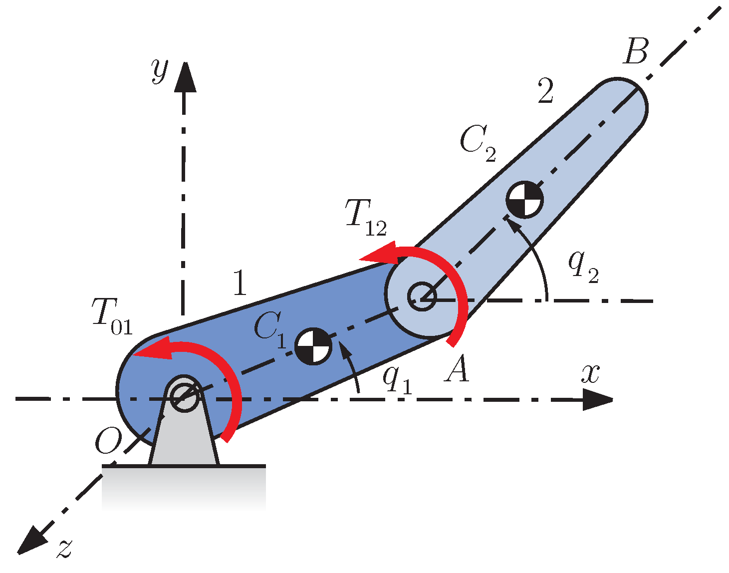
Figure 2.
Impact for the robotic arm.
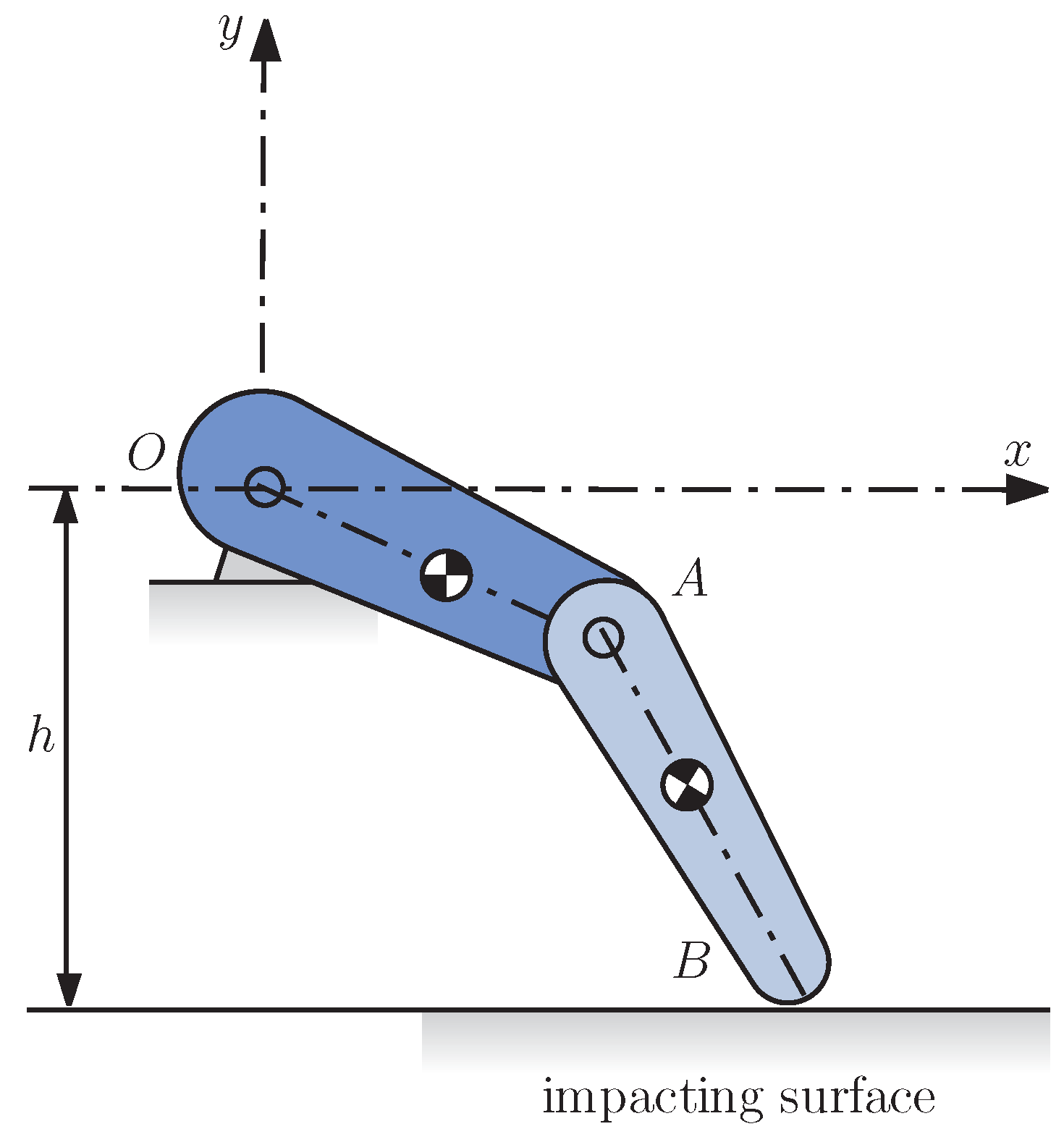
Figure 3.
Comparison of PID controller, Q controller, and PD controller: (a) response of link 1 (b) response of link 2.
Figure 3.
Comparison of PID controller, Q controller, and PD controller: (a) response of link 1 (b) response of link 2.

Figure 4.
Change of link angles with time: (a) angle and (b) angle .
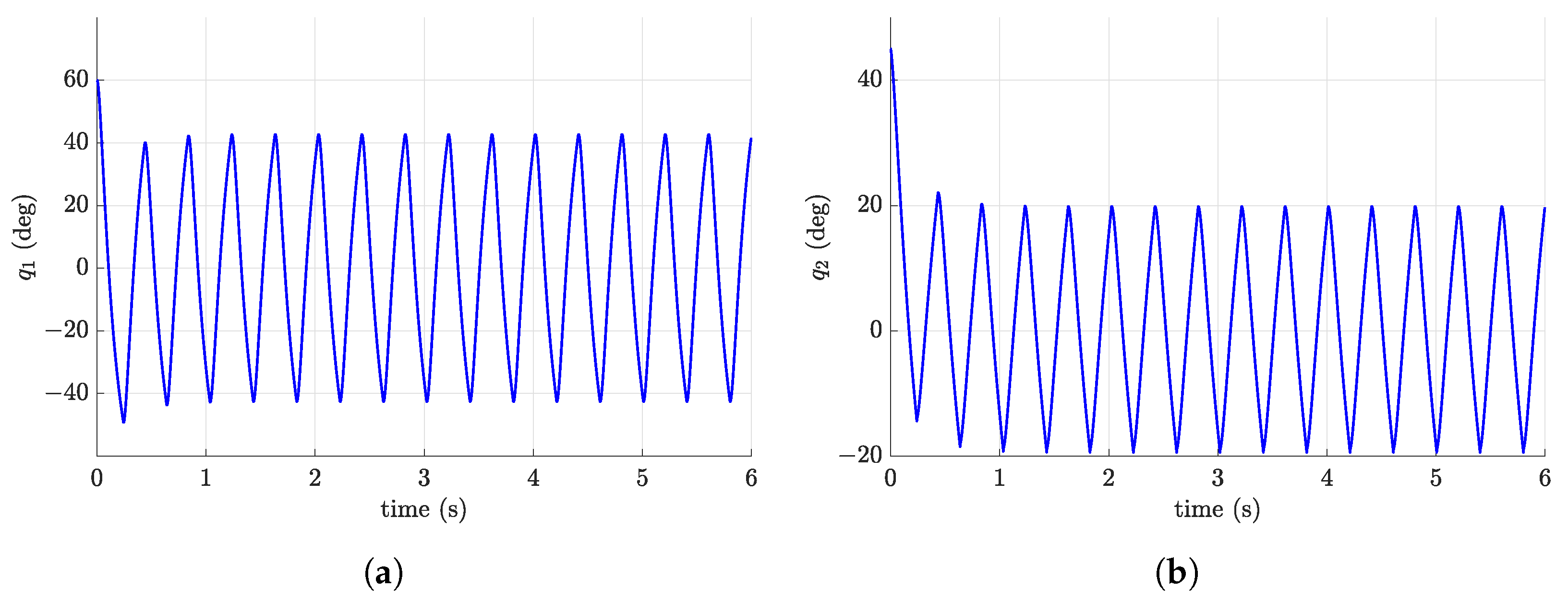
Figure 5.
Phase portraits: (a) , (b) .
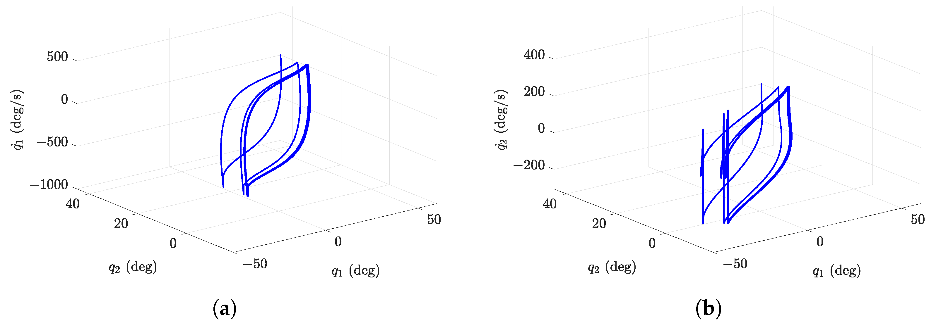
Figure 6.
Poincare maps (a) and for crossing, and (b) and for crossing.
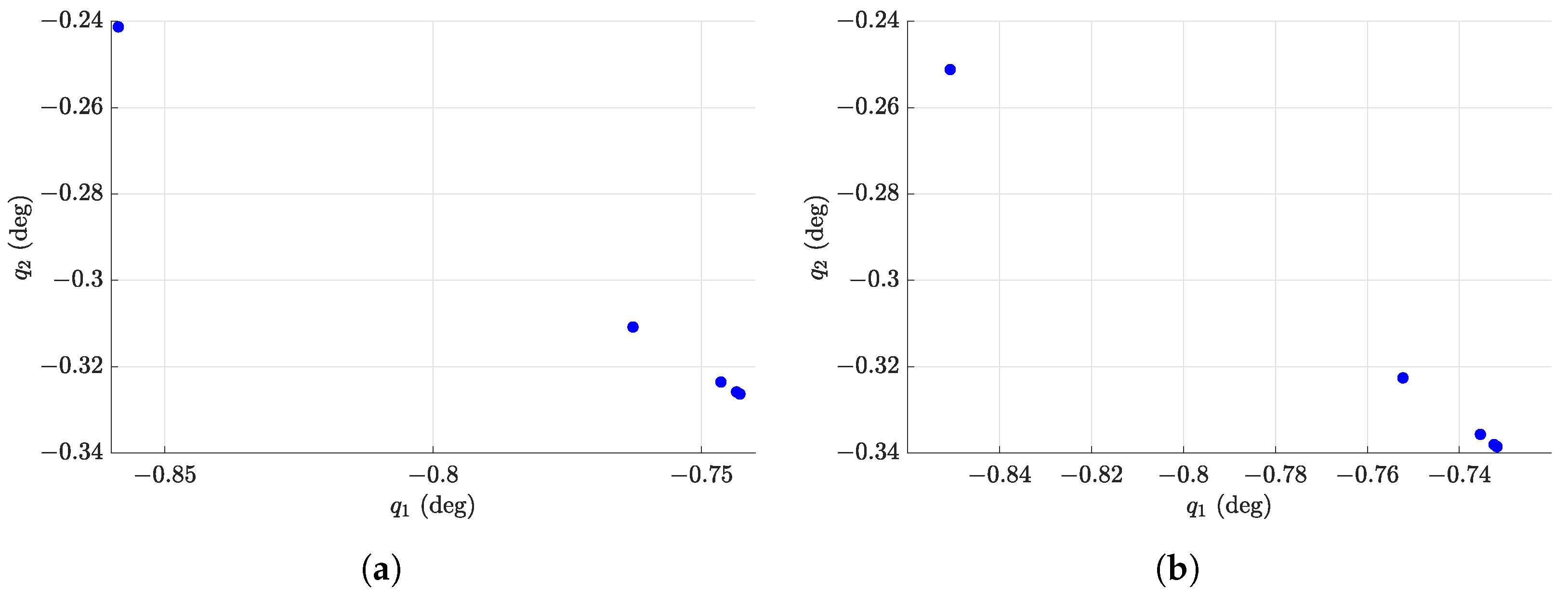
Figure 7.
Velocity of the end effector: (a) velocity on x-axis (b) velocity on y-axis.
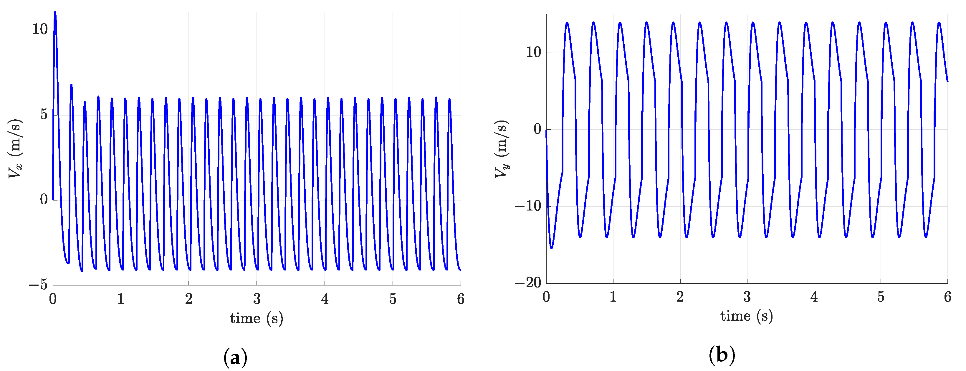
Figure 8.
Indentation during the first impact.

Figure 9.
Velocity of the end effector during the first impact: (a) tangential velocity of impact (b) normal velocity of impact.
Figure 9.
Velocity of the end effector during the first impact: (a) tangential velocity of impact (b) normal velocity of impact.
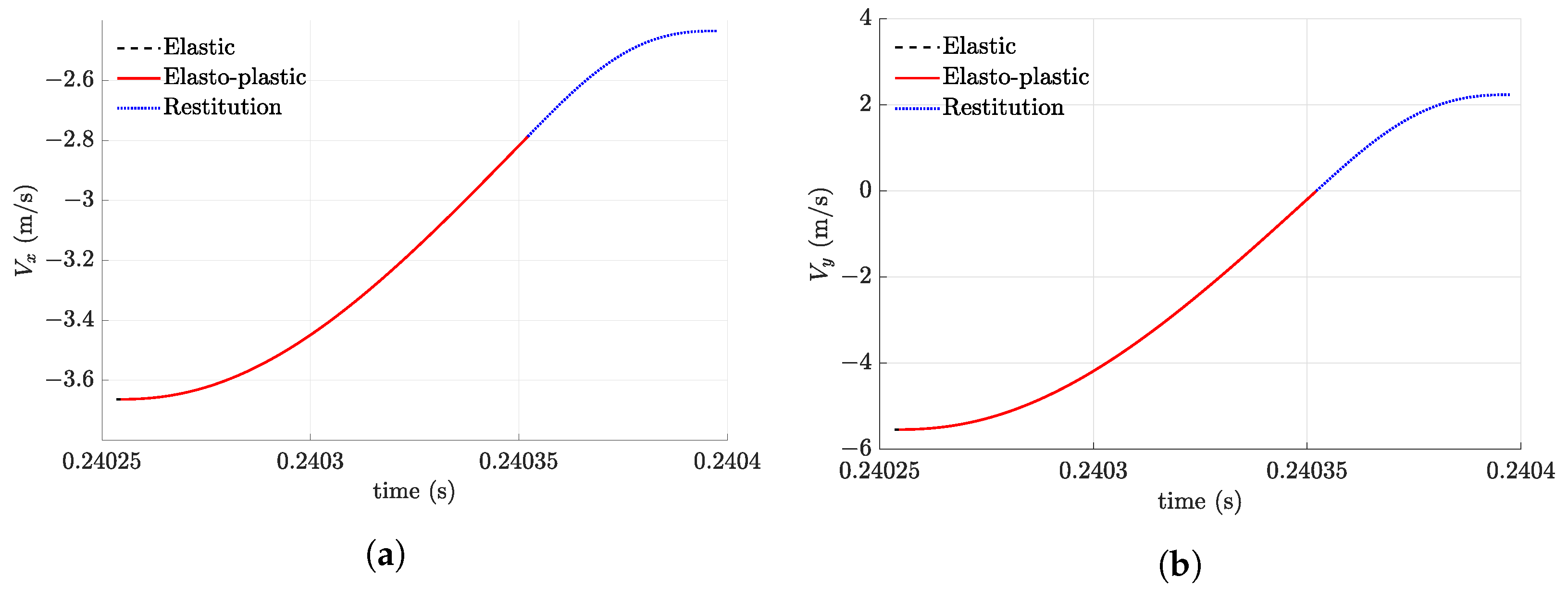
Figure 10.
Contact force during impact.

Figure 11.
Kinetic energy during impact: (a) the kinetic energy of link 1; (b) the kinetic energy of link 2; (c) total kinetic energy.
Figure 11.
Kinetic energy during impact: (a) the kinetic energy of link 1; (b) the kinetic energy of link 2; (c) total kinetic energy.

Table 1.
System parameters.
| Robotic Arm | Fixed Surface | ||
|---|---|---|---|
| 7800 (kg/m) | 7800 (kg/m) | ||
| E | 210 (GPa) | E | 210 (GPa) |
| 0.29 | 0.29 | ||
| 1.12 (GPa) | 1.12 (GPa) | ||
| 0.2 | 0.2 | ||
| L | 1 (m) | ||
| R | 0.005 (m) | ||
| m | 1 (kg) | ||
Table 2.
Control gains, initial position, and target position.
| Control Gains | Initial Position | Target Position | |||
|---|---|---|---|---|---|
| 600 (N m/rad) | |||||
| 300 (N m/rad) | |||||
| 100 (N m/rad) | 0 | ||||
| 100 (N m/rad) | 0 | ||||
Disclaimer/Publisher’s Note: The statements, opinions and data contained in all publications are solely those of the individual author(s) and contributor(s) and not of MDPI and/or the editor(s). MDPI and/or the editor(s) disclaim responsibility for any injury to people or property resulting from any ideas, methods, instructions or products referred to in the content. |
© 2023 by the authors. Licensee MDPI, Basel, Switzerland. This article is an open access article distributed under the terms and conditions of the Creative Commons Attribution (CC BY) license (https://creativecommons.org/licenses/by/4.0/).
Share and Cite
MDPI and ACS Style
Akhan, A.F.; Zhao, J.; Tarnita, D.; Marghitu, D.B. Repeated Collision of a Planar Robotic Arm with a Surface Using Generalized Active Forces. Machines 2023, 11, 773. https://doi.org/10.3390/machines11080773
AMA Style
Akhan AF, Zhao J, Tarnita D, Marghitu DB. Repeated Collision of a Planar Robotic Arm with a Surface Using Generalized Active Forces. Machines. 2023; 11(8):773. https://doi.org/10.3390/machines11080773
Chicago/Turabian StyleAkhan, Ahmet Faruk, Jing Zhao, Daniela Tarnita, and Dan B. Marghitu. 2023. "Repeated Collision of a Planar Robotic Arm with a Surface Using Generalized Active Forces" Machines 11, no. 8: 773. https://doi.org/10.3390/machines11080773
Note that from the first issue of 2016, this journal uses article numbers instead of page numbers. See further details here.