
A Knowledge Discovery Process Extended to Experimental Data for the Identification of Motor Misalignment Patterns


Working Group Electrotechnical Systems of Mechatronics, Kaiserslautern University of Applied Sciences, 67659 Kaiserslautern, Germany
*
Author to whom correspondence should be addressed.
Machines 2023, 11(8), 827; https://doi.org/10.3390/machines11080827
Submission received: 6 July 2023
/
Revised: 4 August 2023
/
Accepted: 8 August 2023
/
Published: 11 August 2023
(This article belongs to the Special Issue Machine Health Diagnosis & Prognosis by Advanced Sensing and Data Driven Techniques)
Abstract
:The diagnosis of misalignment plays a crucial role in the area of maintenance and repair since misalignment can lead to expensive downtime. To address this issue, several solutions have been developed, and both offline and online approaches are available. However, online strategies using a small number of sensors show a higher false positive rate than other approaches. The problem is a lack of knowledge regarding the interrelations of a fault, disturbances during the diagnosis process, and capable features and feature vectors. Knowledge discovery in database is a framework that allows extracting the missing knowledge. For technical systems, optimal results were achieved by aligning (partially) automated experiments with a data mining strategy, in this case classification. The results yield a greater understanding of the interrelations regarding parallel misalignment, i.e., feature vectors that show good results also with varying load and realistic fault levels. Moreover, the test data confirm a specificity (range 0 to 1) for classification between 0.87 and 1 with the found feature vectors. For angular misalignment, potential vectors were identified, but these need further validation with a modified experiment in future work. For the study, two induction motors with 1.1 kW and 7.5 kW were considered. Furthermore, the findings were compared with additional motors of the same rated power. The findings of this work can help to improve the implementation of sensorless diagnostics on machines and advance the research in this field.
1. Introduction
Coupling wear, fatigue cracks, or rotor-to-stator rubbing are the results of improper alignment between an electric motor and its load machine [1]. To avoid costs for repair and unexpected downtime, plant operators need to take care that systems are properly aligned. During the mounting process of a new system or after maintenance, optical approaches are widely used for alignment. Although the process is time-consuming and requires special equipment and know-how, the risk of an accident decreases. Unfortunately, misalignment can also occur during operation through thermal expansion or vibration. In this case, Motor Current Signature Analysis (MCSA) can be applied. This approach uses specific components of the spectrum from motor to the current to recognize a change in alignment. Unfortunately, these components are also related to the load and other faults like broken rotor bars or eccentricity. In real applications, this multi-dependency of the features leads to false positives and poses a serious problem for decision makers. Furthermore, this issue cannot always be solved by installing additional sensors because of higher cost, harsh environmental conditions, and the fact that each component increases the fault risk.
The question is how to improve the quality of an online diagnosis system such that misalignment can be diagnosed based only on electrical signals. Such an improved system needs to consider online diagnosis, minimal false positive indication, and minimal number of sensors, and should be easy to set up. In order to find such a solution, a fundamental understanding of the fault is necessary. Knowledge Discovery in Database (KDD) is an approach that provides sufficient knowledge. According to [2], the KDD process is defined as follows: The process of using the database along with any required selection, preprocessing, subsampling, and transformations of it; to apply data mining methods (algorithms) to enumerate patterns from it; and to evaluate the products of data mining to identify the subset of the enumerated patterns deemed “knowledge”.
In addition, a unified framework for KDD and its objectives are described in [2]. The process was designed to find patterns within the data that are expected to fulfill the needs of an improved diagnosis system as mentioned above. Besides steps for data formatting and data visualization, KDD includes the better known Data Mining (DM) approach, which is the main process. Nevertheless, it is necessary to emphasize that KDD is more than DM because the results are subject to further assessment.
Although the idea of KDD is applied in many research fields, the research in technical diagnostics of rotating machines has been dominated by the validation of expert knowledge, and the implementation of novel classifiers partly in combination with expert knowledge. Both approaches have met the needs in research for a long time. This is why MCSA is one of the best known approaches to implement expert knowledge in this field. An overview of the research in condition-based monitoring, respectively, technical diagnostics, is given in [3], where the literature research is separated into several categories including feature-based approaches and Artificial Intelligence. Examples of research on features are [4,5], who show the effects of misalignment on the motor current spectrum. In addition, ref. [6] compared the MCSA approach with vibration analysis with good results for the analysis of single components within the spectra. This knowledge is sufficient for many applications, but MCSA fails in the case of varying load, as examined in [7]. The reason is that the load affects the same spectral component as misalignment. In addition, various faults also affect the same spectral components as misalignment, as shown in [8]. As a consequence, new concepts were developed that are able to deal with load dependencies. These concepts use new media for calculating the spectra, such as instantaneous power, which was compared with current in [9]. Another alternative is to use load-independent states like the start-up of a machine. This idea leads to Advanced Transient Current Signature Analysis (ATCSA), as examined in [10]. The drawback lies in the fundamental idea of the concept, because a start-up or a similar load-independent state is necessary for a valid classification, which is not always possible during the operation of a motor. Another approach developed in research on technical diagnostics are machine learning algorithms. The power of multidimensional classifiers is shown in [8], where several time-domain features were calculated, and in [11], where features were calculated using an auto recursive model. Furthermore, in [12], wavelet transform was combined with a convolutional attention neural network with good results for multiple faults, but without considering the shift in operational point. Two different motor faults, namely bearing faults and broken rotor bars, were classified in [13] with a convolutional neural network in combination with automated feature extraction. High-quality features were named by [14] as the key to good classification, but they require expert knowledge and human intervention. To solve this issue, deep believe networks have been applied. Although these contributions show the power of modern classifiers, they rather aim to improve the classification process that is based on the known expert knowledge than to find fundamental relationships between (new) features and the target. In addition to the listed literature, some works address these relationships. For example, ref. [15] combined machine learning with expert knowledge of MCSA to extract discriminant features. The motivation was to improve traditional machine learning classifiers because they are less affected by data availability than deep learning models, as investigated in [16]. Although the research showed good results for the classification of different faults, KDD was not applied and the experiments deviate from realistic applications. Thus, no statement regarding the limits of the features was possible. Another suggestion to address the problem of missing data for Artificial Intelligent models was made in [17], with the idea being to gather data provided directly by industrial processes. The incoming data were processed using an anomaly detection to create training data for a classifier. The drawback of this approach is the access to plants and missing process control, which makes the approach reactive and time-consuming, and imbalanced data cannot be avoided. A divergent way that was shown in [18] is inspired by ATCSA. First, a model was used to identify and analyze a detail of the wavelet transform; then pattern recognition was applied on that detail to extract features for classification. The transfer of already gathered knowledge is the objective in [19]. They trained a convolutional neural network and transferred the learned parameters using a transfer learning technique, with the disadvantage that the knowledge is implicit. In a previous work [20], DM was applied on experimental data in order to find a universal feature set for the classification of misalignment. For DM, a pool with general and expert features was created. The result of that work were several feature sets with a classification error below 1%. Although the results of the DM were good, they do not fulfill the needs of a KDD process. In order to achieve knowledge about misalignment, additional steps like visualization and evaluation are needed. For visualization, a survey of different approaches is given in [21]. Furthermore, ref. [22] evaluated a current approach, elliptic paired coordinates, which should allow a lossless depiction of high-dimensional data. The evaluation of the results from DM can be done through 2D interpretation of the results combined with various criteria such as understandability, expressed through the number of features needed for classification, or interestingness, which is a combination of validity, novelty, usefulness, and simplicity. In a current study [23] in the field of technical diagnostics, KDD and DM were used to identify causal insights for the prediction of wearing at the cutting edge of a milling machine. Beyond the field of technical diagnostics, the focus on KDD is higher. For example, ref. [24] applied KDD with different DM techniques (association analysis, sequential pattern mining, and clustering) to find answers for different medical questions. In addition to the applied DM techniques, regression, classification, anomaly detection, and data warehousing were identified.
To overcome the lack of information regarding misalignment and the lack of a research strategy in the field of technical diagnostics, this work contributes an exemplary KDD process aimed at achieving knowledge about misalignment under realistic conditions. The focus is on feature vectors with highly discriminant capabilities for multiple levels of misalignment and without faults in the data structure. In order to achieve causal insights, the KDD framework is extended to include an experiment. The measure has a crucial impact on the whole KDD process when experiment and DM are aligned and interaction between the growing knowledge and the appropriation of new data takes place. Furthermore, the measure fulfills the data science requirement of high-quality data while allowing the number of samples for each class to be increased by automation. In addition, the experiment allows gathering data for both analysis and testing with different machines. The remainder of this paper is organized as follows. In Section 2, the methodology used for the KDD process, the DM, and the experiment is described, while Section 3 presents the results and a discussion of the findings.
2. Materials and Methods
In this section, the methodology for the analysis of misalignment using KDD is presented. In Section 2.1, an overview of the KDD process is given that describes the role of DM and the experiment in the whole process. In Section 2.2, the experiment is described, with details on the experimental setup, the devices used, and the experimental sequence. Section 2.3 and Section 2.4 present the DM process and how it is applied to find fault-related features and interpretable patterns from the experimental data. To this end, DM is divided into two steps, feature extraction and feature selection, which are coordinated with the experiment.
2.1. Knowledge Discovery
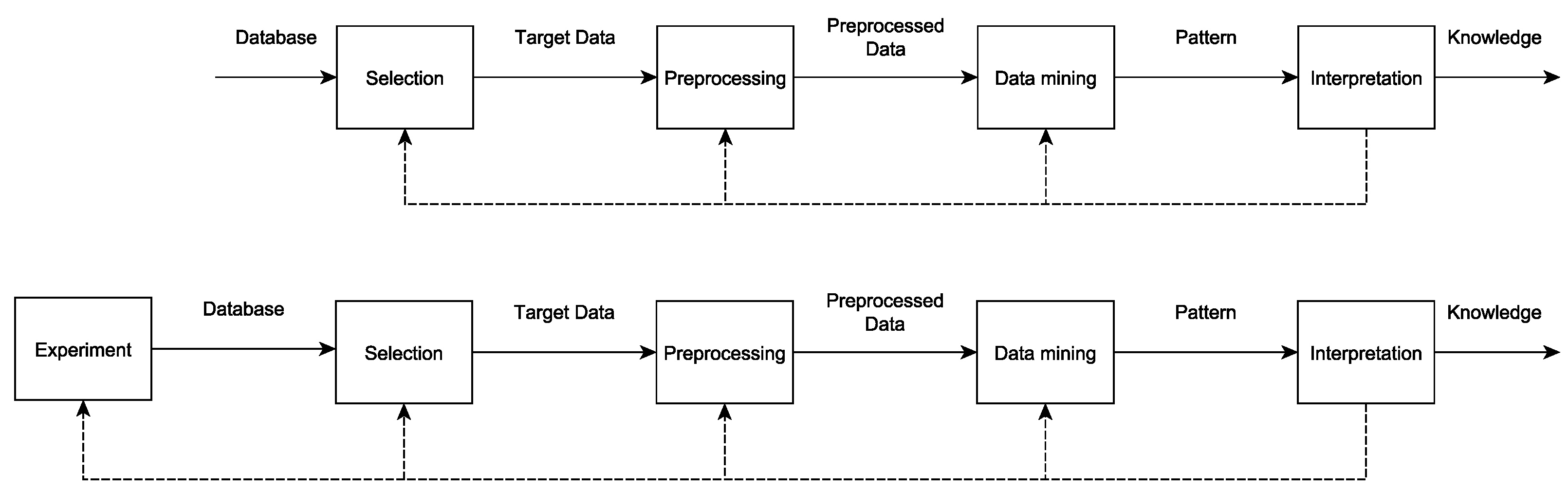
In the following, the applied KDD process is described and discussed. The original framework introduced in [2] is depicted and compared with the suggested framework, which includes the experiment illustrated in Figure 1.
The original framework shows some drawbacks regarding the databases, because not all databases were created to gather the data required for KDD and the collection of additional data is not always possible. As a result, data imbalance could affect the KDD. In the case of technical diagnostics, especially for rotating machines, data can be created through a coordinated experiment. In that case, the same number of samples per class can be collected. Moreover, the number of samples can be set to the acquired amount. In addition, the experiment can be designed for the desired DM technique that is in this case the classification. In order to realize all the requirements, automated or partially automated experiments are needed. A detailed overview of the partially automated experiment is presented in Section 2.2.
After the selection of the target data, preprocessing is applied. In the case of the suggested framework, this includes feature extraction, scaling, and transformation. Feature extraction means applying a metric on a time series or a spectrum that leads to compression of the data and creates interpretable features. A detailed description of the applied feature extraction is provided in Section 2.3. Furthermore, the algorithm selected for the DM requires scaling, which is necessary for algorithms based on distances, transformation, and data combination. While transformation does not play a role in the applied DM, the combination of the data does. Details about the combination of the data are provided in Section 2.4.
In the data mining step, information is extracted from data by applying feature selection. Furthermore, feature selection is well coordinated with feature extraction, which is a crucial part of the discovery strategy. According to [25] these algorithms pull out important features and allow understanding the attributes or variables. There are two types of feature selection algorithms: filter and wrapper. A comparison of the two was conducted in [26] with similar results for accuracy and differences in number of features and computational time. A crucial aspect for the proposed KDD is the characteristic of wrapper-type feature selection, which allows evaluating combined features, as mentioned in [26]. Algorithms such as Ant Colony Optimization (ACO) were developed to search for such feature combinations and are capable of finding the global optimum [27]. The drawback of this kind of algorithm is the search time, especially in combination with big search spaces. One solution is to combine filter and wrapper types. A systematic approach for identifying the signal-generating processes of a time series is presented in [28]. The methodology considers multiple sources with different periods, which leads to a combination of filter- and wrapper-type feature selection.
The interpretation of the results from the data mining step is the key part of KDD. In this step, the enumerated results are checked for useful patterns that will allow interpretating the relationship between the target (misalignment), the disturbance (load), and the features for the diagnostics. An automated KDD process can find so many results in a large database that a human cannot process them. Because of this, one measure within the interpretation step is to limit the number of results. In order to do this in an automated process, a criterion is applied. In the literature, different criteria are defined; for example, understandability, validity, novelty, usefulness, simplicity or the overall measure interestingness as in [29]. The applied data mining algorithm is configured to enumerate all feature sets that achieve a given error rate. For the interpretation of the results, simplicity is selected to shrink the overall number. The criterion is defined as:
where m is the number of features of a feature vector, D is the number of disturbances, and 1 stands for the target. The number of disturbances depends on the expected effects on the system that is undergoing technical diagnostics. In the experiment conducted, the number of disturbances was one because only the load was considered. This means that only feature vectors with two features are interpreted. Thanks to the selected criterion, the second goal of preparing the visualization is easy, since no processing is needed. In all cases where the feature vector has more than two dimensions, a strategy for visualization is needed.
2.2. Experiment
This part details the experiment that was conducted to acquire the data used for KDD, including testing with additional data. The original experiment was developed in [20] with the aim of applying DM. As described above, DM is just one step in the whole KDD process and cannot lead to valid knowledge, as the interpretation of the results from the previous work showed. Some of the identified issues with previous results need to be addressed by the design of the experiment, mainly regarding the definition area of the measured states. In addition to the original experiment, data with a smaller scope was gathered with additional machines to assess the results.
The experiment was designed to acquire data for fault misalignment, which is a displacement between the rotational axis of the motor shaft and the load machine shaft. This displacement leads to the above-mentioned issues when the machines are coupled. There are two types of misalignment, parallel misalignment (PM) and angular misalignment (AM). In the case of PM, the rotational axes are parallel but do not intersect. In the case of AM, the rotational axes are not parallel.
2.2.1. Experimental Set-Up
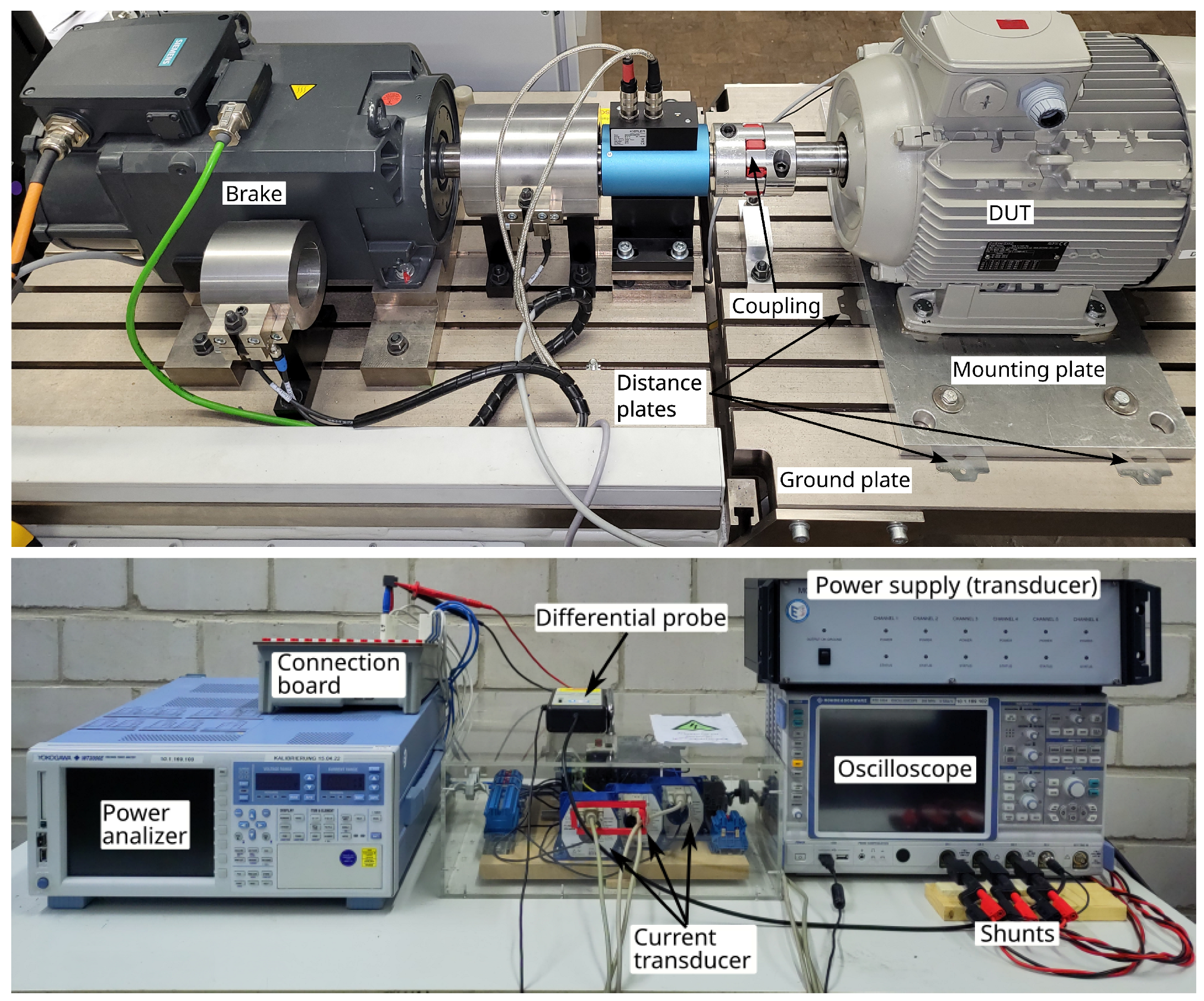
In order to set up multiple types and levels of misalignment in combination with different load levels, a motor test bench was used. As depicted in Figure 2, the misaligned motor, called device under test (DUT) in the following, was coupled with a brake using a claw-type coupling. The brake was an induction motor (IM) with 7 kW rated power and a control system that allows varying the torque. During operation, the DUT was powered by the mains and mounted on a mounting plate that allowed alignment and misalignment only in one dimension, while the positions in the remaining dimensions were forced. The forcing was realized through a check rail and a body stop.
The experiment comprised PM and AM. The misalignment type and the level for each DUT could be set through distance plates between the mounting plate and the ground plate. For this purpose, distance plates with different thicknesses were combined, with the smallest one being 0.025 mm, and placed at the front and rear of the DUT. Diverse devices were used for acquiring data. The measurement equipment was divided into three categories with the following objectives:
- Measurement of signals for data processing
- Offline acquisition of misalignment for quality management
- Online acquisition of process signals for quality management
For the measurement of the signals for data mining, a four-channel oscilloscope (Rohde&Schwarz RTE 1034) with a sample frequency of 10 kHz was used. With this device, three terminal currents of the DUT were measured via current transducers (LEM IT 200-S Ultrastab) and shunts (Yokogawa 19/SH5/BNC/0.05). The fourth channel was used to measure one line-to-line voltage via a differential probe (Rohde&Schwarz RT-ZD01). To ensure the quality of the experiment, additional information was acquired. The levels of misalignment were measured after each adjustment with an optical alignment system (easyLaser XT660) with a resolution of 0.001 mm for PM and for AM. It must be noted that AM is the gap at the outer distance of a coupling with a diameter of 100 mm. The set-up of devices can is shown in Figure 2. During the operation of the motor, several process signals were observed for quality management purposes: input power via a power analyzer (Yokogawa WT3000), speed and torque via a torque measurement shaft (Kistler 4503A50L), as well as environmental and motor temperature via a temperature probe (Texas Instruments LM35DT). Additional information about the sensors used is given in Table 1.
2.2.2. Scope of the Experiment
With the set-up described above, 42 states were created as a combination of the following parameters:
- Motor size (kW): 1.1 and 7.5
- Load (% of rated power): 100–92, 90–82, 80–72
- Misalignment (mm): aligned = 0.02 (PM, AM), 0.05 (PM), 0.08 (PM), 0.11 (PM), 0.05 (AM), 0.08 (AM), 0.11 (AM).
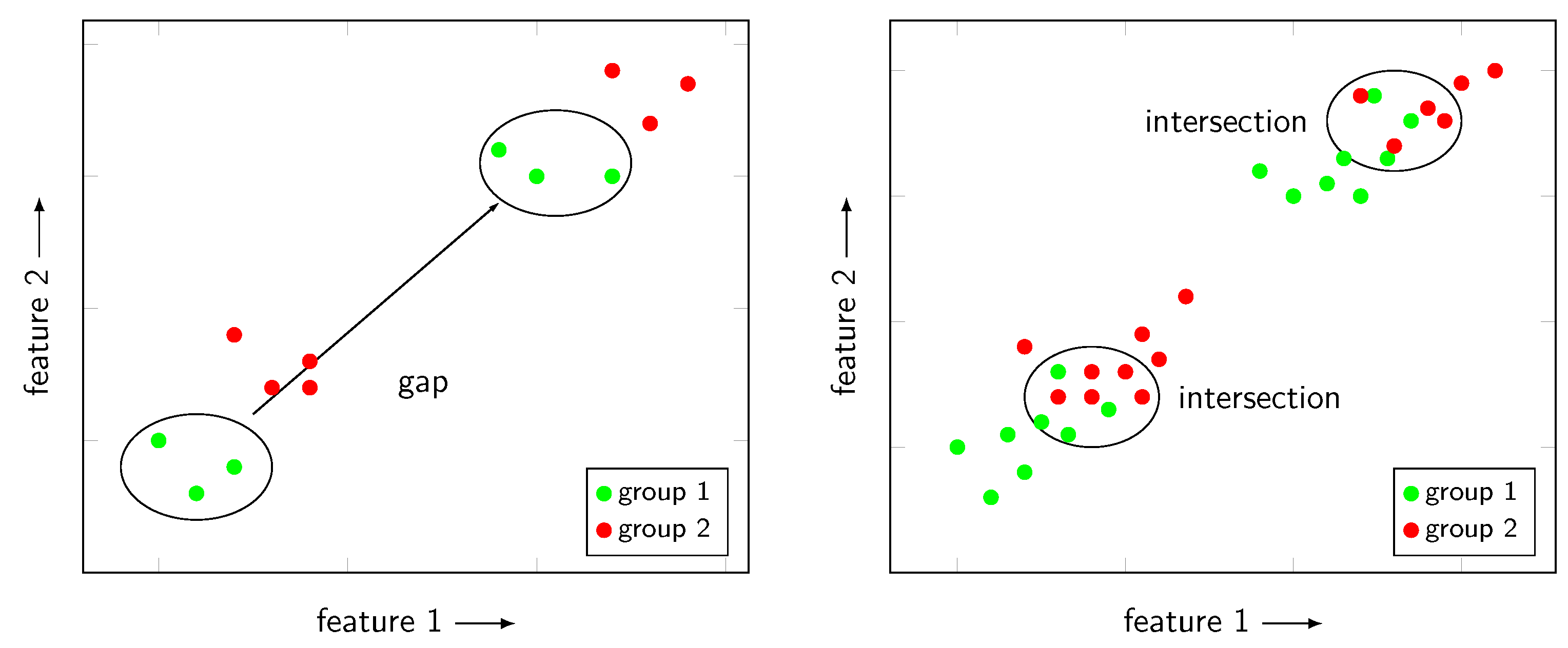
The experiment included two motors of the same type (four-pole IM). With each motor, 21 states were created as a combination of misalignment and operational point, i.e., load. These measured states are primary classes that can be combined to create new classes containing a variation of a parameter. The variation within a class allows searching for features that are independent of the varying parameter. Regarding the load, several modifications were made compared to the previous work. The first optimization regarded the location of the states and thus the primary classes. An analysis of the previous results had shown that automated feature extraction based on MCSA might fail to select the right peak if the dominant peaks are crowded and spectral leakage occurs due to a bad signal-to-noise ratio. In order to improve the reliability of the feature extraction, the operational points were moved close to the rated power; 100%, 90%, and 80% of the rated power were selected. Due to this measure, no drawbacks were expected for the KDD process because the dominant effects should be captured. For the results to be applicable, it needs to be checked whether the features can be used at partial load or whether noise becomes dominant. The second optimization was to take into account continuity of the load and the DM with a classifier. In the previous experiment, only samples with a small definition area around the defined operational points were considered. That allowed distributed clusters of one class and settlement of other groups in the gaps. This problem and the solution are depicted in Figure 3. Such feature sets achieve low classification errors but will fail in real application. The measures applied to avoid such a selection, included defining an operational area instead of an operational point and using small step sizes to close the gaps between the classes/states. This led to states with an eight percentage points definition area of the load and two percentage points distance to the next state. An alternative could be the application of a regressor instead of a classifier in the DM step. This idea was discarded as it would have required substantial modifications in the data processing, but will be the subject of future work.
The values for PM and AM were derived from a best practices guide (handbook of OPTALIGN smart RS5) for shaft alignment published by Prueftechnik, a producer of optical shaft alignment systems; see Table 2.
Due to the selected parameter variation, it is not possible to create a case to search AM with PM as disturbances and vice versa; see Section 2.4. The examination of the faults had to be separate. Note that even with an optical shaft alignment system and distance plates of 0.025 mm, the states of PM can have an unwanted amount of radial misalignment and the states of AM can have an unwanted amount of parallel misalignment. In order to shrink the unwanted effect, a threshold of mm for PM and for AM was defined.
The experiment with 42 states was conducted twice. In the first round, data was acquired for mining and in the second round for testing. Both rounds differed in the scope of the data, which was higher for analysis, while additional DUTs were used for testing. In the first round, 50 signal samples with a length of 100 s for each state were acquired, which led to a total measurement time of approximately 60 h without adjustments. For testing, the number of samples for each state was decreased to 125. The experimental cycle comprised three measures of adjustment, as depicted in Figure 4.
The first step was to align the DUT without any distance plate between the mounting plate and the ground plate. This step also included correction of the soft foot, meaning that the motor feet with four connection spots only touch the ground in three spots. This is due to manufacturing tolerances and leads to bracing of the housing if all connection bolts are tightened. Without compensation, the alignment is not controllable. After alignment, the DUT ran at the rated load until a steady state temperature was reached. With this measure, the influence of temperature on the data should be avoided because temperature is not declared as a dominant influence. This step was followed by measurement of the mentioned quantities. Then the load was decreased automatically in 75 steps, 25 steps per group, and the next measurement started without temperature correction. Once all load variations had been measured, the level of misalignment had increased. The earlier steps were repeated until all states were set, then the next DUT was mounted.
2.3. Feature Extraction and Preprocessing
Feature extraction is the process that creates or extracts features from signals. With this measure, the data is compressed while the degree of physical interpretation increases. With feature extraction, a feature stock is created from which a feature selection algorithm selects the combinations of interest. The feature stock benefits from both general metrics and expert features derived from MCSA. The process applied and some examples of the feature extraction are depicted in Figure 5.
As shown, there are three steps: calculation of virtual sensors, transformation, and application of a metric. A feature extractor is defined by the algorithms applied in each step, respectively, by whether any algorithm is applied at a step. All combinations lead to five feature extractors, which were applied to the collected data (see Section 2.2):
- 1.
- Time-domain features extractor
- 2.
- Space vector time-domain features extractor
- 3.
- Frequency-domain features extractor
- 4.
- Space vector frequency-domain features extractor
- 5.
- MCSA features extractor.
In addition to the above-mentioned steps, preprocessing of the data took place. This step is not part of the feature extraction but determines how many samples of each feature are available for DM and testing. Based on the experience gathered in the previous study, 1000 is an adequate number of samples. For the first four extractors, that number was achieved by splitting each signal with a length of 100 s into 5 s sequences. In the case of the MCSA features, the original 100 s were split into 25 s. This is because previous analyses had shown that a higher spectral resolution is needed for correct automated peak selection after the calculation of the harmonic. The different numbers of samples were adapted by cloning each sample of the MCSA extractor five times. In the case of the extractors that process data with the Fourier transform, the Hann window was applied and the spectra was scaled with the fundamental frequency and then expressed in decibels. The window function improved the determination of the correct feature values by suppressing the leakage effect, while the scaling emphasized the relevant components of the spectra.
Time-domain features were calculated after preprocessing by simply applying different metrics to describe signals or statistical distributions, such as root mean square or rectified value.
Space vector time-domain features were calculated in the same way as the time-domain features, but the metric was applied to different signals coming from the space vector transform. The signals used were:
- Length of the space vector
- Angle of the space vector
- Fluctuation of the space vector length
- Fluctuation of the space vector angle [30].
All signals were derived from the space vector components in polar coordinates, which were calculated at every point in time.
Unlike the time-domain features, the frequency-domain features were calculated after a Fourier transform. The resulting spectra were then split into 20 segments in order to get a deeper search. This was done because features were calculated based on the input, which could be the full spectrum or only a single band. If the input is the full spectrum and the automated feature extraction algorithm searches for the peak value, it would always find the fundamental component. By segmenting the spectrum, peaks could be determined for twenty bands. The number of features from the spectrum increased by a factor of twenty. The extractor uses statistical metrics and searches for the first five highest peaks and their position within the band.
Space vector frequency-domain features were processed in the same way as frequency-domain features. The process was only applied to the virtual sensor signals from the space vector transform.
MCSA features were calculated in the same way as fault-correlated frequencies and their amplitudes were calculated according to MCSA as in [5]. In addition, the slip, the winding harmonics, and the principal slot harmonics were calculated. In the first step, the Fourier transform was applied and then the equations from MCSA were applied to find the position of the fault-correlated frequency. In order to avoid any loss of information, all orders within the spectra were calculated.
After automated creation of the feature stock, preprocessing is necessary to make the data suitable for DM, respectively, feature selection. The first process was normalization with z-score, which uses the variance to scale the features. This measure is necessary if distance-based classifiers are to be applied. The second step was data cleaning, were non applicable features and samples with forbidden numeric values like infinity and not a number, were deleted. These values can be a result of automated feature extraction, especially in the case of the expert features for which automated peak selection was applied. Moreover, all features with a variance equal to zero were deleted. No further transformation of the data was applied.
2.4. Feature Selection
The second step in DM is feature selection, which will be described in the following, including the algorithms used and the cases examined.
The selected feature selection algorithm was a wrapper-type, bottom-up algorithm that sequentially adds features in order to reduce the failure rate. For the classification, a k-nearest neighbors (kNN) classifier with was used. The kNN classifier was applied because of the simple training and approximation, and the low number of parameters. The drawbacks such as storage usage and slow approximation can be neglected for the KDD process. The parameter k was found by a trial-and-error strategy for which enumerated feature vectors were used as optimization criterion. In order to avoid over-fitting, the classifier was embedded into 10-fold cross-validation. The validation algorithm calculates the average of the error rate over ten turns with a random selection of samples for training and classification. The building of the feature vector stops when an error rate below 1% is reached or if there is no progress.
In order to find features for different cases, new classes were created by merging and combining several primary classes. The new classes were then processed by the feature selection. Each case can be described with three parameters: target (T), restriction (R), and disturbance (D). For all parameters, one of four quantities describing a primary class, respectively, a state, are possible: PM, AM, load, and motor size. The target parameter decides which quantities are to be classified, while disturbance is an unwanted but unavoidable influence. Both parameters need to vary in the resulting class. Restriction limits the variation of a disturbance to a single value, whereby the search space is reduced. The following values are possible:
- Target: parallel misalignment, angular misalignment
- Restriction: DUT 1, DUT 2 (motor size)
- Disturbance: load.
For each of the defined cases, 15 feature selection iterations were conducted. With every iteration, the feature stock is reduced by the previously found features. This measure was applied due to two issues: redundant features within the feature stock and irrelevant features likely to be selected by the algorithm. In order to deal with these issues, it is necessary to enumerate all results that fulfill the defined criterion and to interpret all findings. A drawback of the suggested approach is that important features might only be available once, and thus some feature combinations cannot be found. In order to solve this problem, a postprocess was proposed that uses ant colony optimization, but this did not lead to any improvement.
3. Results
In this section, the findings for the four described cases will be discussed. The findings will be discussed in two subsections starting with the results for PM in Section 3.1 and followed by those for AM in Section 3.2.
Each discussion of the enumerated feature vectors is preceded by a short table showing the Pearson correlation and the error rate for both the analysis and the testing data. It lists only the discussed feature vectors that achieved the lowest error rate with two features, as claimed by Equation (1). A complete list of all feature vectors can be found in Appendix A.
The correlation coefficient gives first insights into the data and helps to understand the selection. In addition to the correlation between the feature and the target as well as between the feature and the disturbance, the correlation between the feature and the unwanted type of misalignment is given. This is because the experimental design did not fully avoid mixed misalignment. In the second step, a selection of interesting feature vectors will be visualized in order to assess the patterns and the behavior of the analysis and test data.
3.1. Parallel Misalignment
In the following, the feature vectors for PM of a 7.5 kW motor will be discussed. A selection of the enumeration of the results from the DM are listed in Table 3.
The complete table only lists the first 10 feature vectors chosen by the feature selection algorithm, i.e., those with the lowest error rate. The enumeration shows features calculated by the Signal, the Space Vector Signal, and the MCSA feature extractors. It can be observed that the feature selection combined a highly load-correlated feature with a highly PM-correlated feature in order to achieve a good classification with an error rate below 1%. Regarding the correlation coefficients and the error rate, the results were confirmed by the test data. The enumeration contains features like ECC1, ECC2, which are known to correlate with eccentricity, and BB2, which correlates with a broken rotor bar. As they are all sensitive to changes in air gap magnetization, their occurrence is expected. In addition, the results show the load and AM dependency of all features correlated with PM. The observation supports the assumption that combined features are needed for reliable diagnostics. Although the results are as expected, it is not possible to transfer the findings to the smaller machine with 1.1 kW. In order to find an explanation for this, the patterns need to be assessed in detail. As described above, visualization and assessment are crucial steps in KDD. Some interesting results will be examined in the following.
Figure 6 shows the first example from the findings with the best possible classification, meaning an error rate of zero.
It can be seen that the samples form well-structured clusters without any intersection. Furthermore, each of the 12 primary classes can be seen in the two selected dimensions. In the direction of the load-correlated feature, the gaps of two percentage points, set during the experiment, occur between all primary classes. In the direction of the misalignment, the gaps vary. This behavior can be explained by the different levels of misalignment during the adjustment. When studying the test data, the same patterns can be recognized. The only remarkable difference is the location of the samples in the direction of the misalignment-correlated feature. In order to explain this observation, the values for misalignment need to be considered. Doing so reveals that for the analysis data, the level of misalignment was lower and led to a smaller degree of damping. For the test data, sensitivity equals 1 and specificity equals 1. Similar results could be achieved with each of the three terminal currents and the MCSA-ECC1 equation.
Another alternative to the feature sets presented above is depicted in Figure 7.
Although the pattern is similar, the classification performance is worse. The feature set uses speed to deal with the load. This is why the pattern is mirrored compared to Figure 6 because the speed is inversely proportional to the load, as also expressed by the correlation coefficients. The worse classification performance can be explained by the approach applied for speed estimation. The speed was calculated using the principal slot harmonics in the spectra with automated peak selection, which can fail in some cases, resulting in diffuse primary classes and outliers. Nevertheless, the finding is that calculating the speed via the principal slot harmonics can improve the implementation of technical diagnostics. The comparison of the patterns with the test data shows the same behavior as discussed above. For the test data, sensitivity equals 0.978 and specificity equals 0.975.
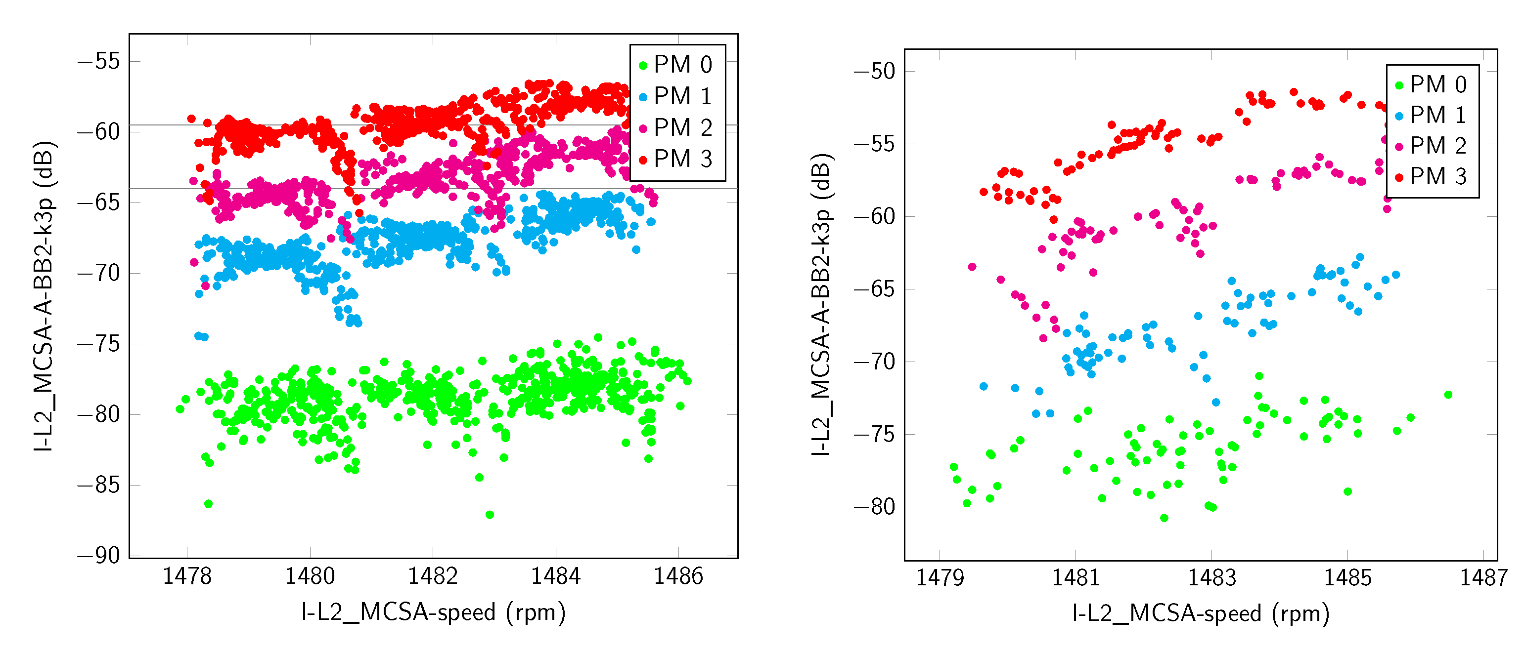
A divergent pattern with a validation error of 0.74% is shown in Figure 8.
In comparison to the feature vectors depicted above, this one leads to four clusters that intersect at their borders. The primary classes cannot be seen, but a sequence of the misalignment levels is visible. It is also remarkable that PM 0 and PM 2 show a wider stray for the shape factor. Furthermore, compared to the other results, both features are correlated with AM, but the shape factor has an inverse sign. The test data are comparable with the analysis data. They both show the same clustering and the same sequence of the misalignment. Differences can be observed in the classes PM 0 and PM 2, for which the cluster shows a smaller stray for the shape factor. A comparison with the level of misalignment during the experiment does not show any anomaly. For the test data, sensitivity equals 0.845 and specificity equals 0.87.
The next case assessed is PM of a 1.1 kW motor with a selection of the enumeration depicted in Table 4.
There are only five feature vectors that achieve an error rate below 5%, and the selection deviates from the previous one. In this case, the features were calculated with the Spectrum and the Space Vector Signal feature extractors. In all selections, the length of the space vector is used to deal with the load. For PM, different peaks were identified, with low correlation with the target compared to the previous case. The pattern discussed later will show a non-linear trend of the feature. In order to discover such patterns it is necessary to avoid filters in the preprocess. Regarding the load, the test data confirm the findings, but in the case of PM, the values differ. A comparison between the levels of PM and AM for the measured states does not show any anomaly.
In order to gain a better understanding of the selected feature vectors and the data, some examples will be discussed. Figure 9 shows the first selection.
With this pattern, it is possible to identify all primary classes that have clear borders without intersection that show a sequence of the PM level. What is remarkable is the arrangement of the data for PM 0 and PM 2 close to the rated load. The observed behavior is the reason why the correlation coefficients are worse, but the error rate is adequate. This finding illustrates why a classifier is used to find potential feature vectors. This behavior cannot be observed with the test data. Also, if the level of misalignment differs by approximately 0.006 mm and the unwanted influence of AM difference is , the reason for the strong increase is not clear. A possible explanation is given in [9], where the influence of rigidness on the correlation between instantaneous active power and alignment angle is shown. Overall, the test data show a plausible arrangement of clusters. With KDD, it was possible to identify an interesting effect for technical diagnostics. Further adjustments of the experiment will clarify whether the observation was induced by the experiment or by a characteristic of the machine. For the test data, sensitivity equals 1 and specificity equals 1.
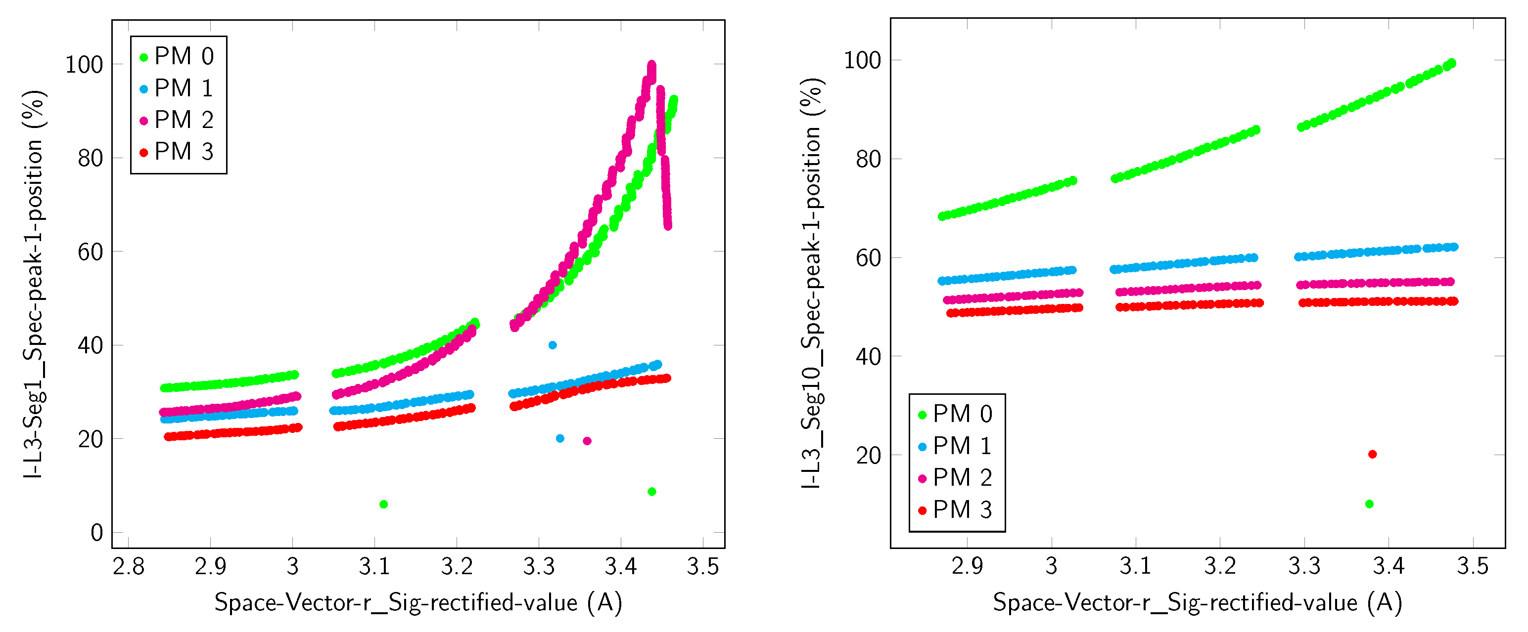
Similar results were achieved with the feature set depicted in Figure 10.
The major difference is that for the analysis data, the peak for PM 3 lies outside the observed segment. The observation reveals an issue with the definition of the segments. If the origin of a moving peak lies close to the borders of the segment and moves outside because of the definition area, the feature is useless since not all information is included. For KDD, this means extending the segments, which has the drawback that other peaks are covered. Another strategy is to align the center of the segment with the location of the winding harmonics, which are mostly the origin. For the test data, sensitivity equals 1 and specificity equals 1.
3.2. Angular Misalignment
The third case is AM of a 7.5 kW motor. A selection of the enumeration of the feature vectors is depicted in Table 5.
Listed are all feature vectors that achieve an error rate below 5%. For this case, only features from the Signal and the Space Vector Signal were selected. It can be seen that only one of the six results shows a correlation between 0.47 and 0.85, while the rest is below 0.05. This result calls for a detailed view on the data. Unfortunately, none of the enumerated results can be accepted. The first selection with the highest correlation between the feature and the AM shows neither a sequence of the AM levels nor the primary classes.
A more interesting pattern is shown by selection 2, which is depicted in Figure 11.
The pattern shows a clear separation of the primary classes with the same load, but the classes intersect. A detailed analysis shows that the reason for the low error rate is the issue with gaps described in Section 2.2.2. Due to the fact that this issue still occurred even after reducing the step sizes for the load, it is unclear whether a diagnosis of AM is possible based only on electric signals. It appears that AM does not have an effect on any characteristic feature and only small effects on the load of the machine. For the test data, sensitivity equals 0.239 and specificity equals 0.102.
Finally, the case of AM of a 1.1 kW motor will be discussed. An overview of some results is shown in Table 6.
In this case, too, the enumeration only shows the results that achieved an error rate below 5%, which were only four feature vectors. Nevertheless, compared to the bigger motor with 7.5 kW, more features correlating with AM are listed. Considering the discussion above, this is a hint that the step size of the load was too big for the larger motor and was only suitable for the smaller one. A future iteration of KDD with adjustments made within the experiment will clarify this.
Figure 12 depicts the pattern of the first selection, which is similar to the other selections.
With this pattern, all primary classes can be seen, but there is an intersection especially close to the rated load. This pattern is similar to Figure 9 except for two observations: In the case of the analysis data, the second level of misalignment also intersects the other groups; in the case of the test data, the sequence of the groups is not adequate, as misalignment levels one and two are interchanged. The fact that the same features were found as for PM means that it is not possible to distinguish between PM and AM using this data set. In addition, the correlation coefficients show a relationship between AM and PM. In order to clarify this, a new experiment is needed that considers mixed types of misalignment so that the KDD for misalignment has to consider PM and AM as a dominant influence. For the test data, sensitivity equals 1 and specificity equals 1.
4. Discussion and Outlook
With this study, it was possible to show the power of KDD in the context of technical diagnostics and misalignment. Using the proposed KDD process, it was possible to enumerate several load-independent feature vectors for diagnosing PM of a 7.5 kW motor, taking the causal dependencies into account for the final selection. In addition, the selection could then be confirmed with independent test data measured on a different machine. The findings can now be used to implement or improve the technical diagnostics for AM of an electric machine.
Further important results were achieved with the other examined cases. Although no clear patterns for PM of the 1.1 kW motor and for AM were found, promising feature vectors were identified during the examination. To clarify the interrelationships, further improvements of the experiment and the KDD process were also identified. It was found that, despite the implementation of small step sizes for the load, the patterns still showed gaps in the case of AM. This observation leads to the assumption that the effect of AM is smaller than that of to PM.
During the design of the KDD process, simultaneous declaration of PM and AM as a dominant influence was excluded, but the data show that features correlate with both. Tolerance for a small portion of the unwanted magnitude is not sufficient to understand all findings. The solution is to consider these dependencies within a new experimental design. This represents one of the benefits of including the experiment in the KDD definition, as this enables additional possibilities during exploration.
KDD has been shown to be an important framework for research in the field of technical diagnostics. It helps to use data from experiments or the field in combination with already available knowledge of electric machines to find rules for different cases of technical diagnostics.
Author Contributions
Conceptualization, S.B. and S.U.; methodology, S.B.; software, S.B.; validation, S.B.; formal analysis, S.B.; investigation, S.B.; resources, S.U.; data curation, S.B.; writing—original draft preparation, S.B.; writing—review and editing, S.B.; visualization, S.B.; supervision, S.U.; project administration, S.U.; funding acquisition, S.U. All authors have read and agreed to the published version of the manuscript.
Funding
This research was funded by the German Federal Ministry of Education and Research (BMBF) grant number 03IHS254A.
Data Availability Statement
Data sharing is not applicable to this article.
Conflicts of Interest
The funders had no role in the design of the study; in the collection, analyses, or interpretation of data; in the writing of the manuscript; or in the decision to publish the results.
Abbreviations
The following abbreviations are used in this manuscript:
| IM | Induction Motor |
| MCSA | Motor Current Signature Analysis |
| KDD | Knowledge Discovery in Database |
| DM | Data Mining |
| DUT | Device Under Test |
| PM | Parallel Misalignment |
| AM | Angular Misalignment |
Appendix A

Table A1.
Complete list of results for parallel misalignment of the 7.5 kW motor.
| Feature Extractor | Metric | Error Rate (%) | Correlation (1) | ||||||
|---|---|---|---|---|---|---|---|---|---|
| Analysis | Test | Analysis | Test | ||||||
| Load | PM | AM | Load | PM | AM | ||||
| Selection 1 | |||||||||
| MCSA () | BB2 (k1+) | −0.087 | 0.962 | 0.619 | −0.23 | 0.929 | 0.808 | ||
| Signal () | SRM | 0.96 | 0.011 | 0.045 | 0.962 | 0.002 | 0.009 | ||
| complete vector | 0 | 0.17 | / | / | / | / | / | / | |
| Selection 2 | |||||||||
| MCSA () | ECC1 (k1-) | −0.087 | 0.962 | 0.619 | −0.23 | 0.929 | 0.808 | ||
| Signal () | SRM | 0.962 | −0.007 | 0.003 | 0.962 | 0.01 | 0.007 | ||
| complete vector | 0 | 0.17 | / | / | / | / | / | / | |
| Selection 3 | |||||||||
| MCSA () | ECC2 (k1-) | −0.087 | 0.962 | 0.619 | −0.23 | 0.929 | 0.808 | ||
| Signal () | RV | 0.962 | −0.008 | 0.003 | 0.962 | 0.015 | 0.011 | ||
| complete vector | 0 | 0.17 | / | / | / | / | / | / | |
| Selection 4 | |||||||||
| MCSA () | BB2 (k1+) | −0.094 | 0.965 | 0.61 | −0.237 | 0.956 | 0.828 | ||
| Signal () | SRM | 0.958 | 0.033 | 0.01 | 0.962 | −0.005 | −0.001 | ||
| complete vector | 0 | 0 | / | / | / | / | / | / | |
| Selection 5 | |||||||||
| MCSA () | ECC1 (k1-) | −0.094 | 0.965 | 0.61 | −0.237 | 0.956 | 0.828 | ||
| Signal () | RV | 0.958 | 0.035 | 0.013 | 0.962 | −0.005 | −0.001 | ||
| complete vector | 0 | 0 | / | / | / | / | / | / | |
| Selection 6 | |||||||||
| MCSA () | ECC2 (k1-) | −0.094 | 0.965 | 0.61 | −0.237 | 0.956 | 0.828 | ||
| Signal () | MS | 0.958 | 0.036 | 0.016 | 0.961 | −0.006 | −0.003 | ||
| complete vector | 0 | 0 | / | / | / | / | / | / | |
| Selection 7 | |||||||||
| MCSA () | BB2 (k1+) | −0.098 | 0.968 | 0.59 | −0.249 | 0.953 | 0.838 | ||
| Signal () | RMS | 0.962 | −0.01 | 0.001 | 0.962 | 0.02 | 0.014 | ||
| complete vector | 0 | 0 | / | / | / | / | / | / | |
| Selection 8 | |||||||||
| MCSA () | ECC1 (k1-) | −0.098 | 0.968 | 0.591 | −0.249 | 0.953 | 0.838 | ||
| Signal () | MS | 0.961 | −0.01 | 0.001 | 0.961 | 0.02 | 0.015 | ||
| complete vector | 0 | 0 | / | / | / | / | / | / | |
| Selection 9 | |||||||||
| MCSA () | ECC1 (k1+) | −0.139 | 0.96 | 0.576 | −0.254 | 0.947 | 0.826 | ||
| Space Vector (r) | SF | −0.254 | −0.396 | −0.432 | −0.063 | −0.619 | −0.433 | ||
| complete vector | 0.742 | 6.13 | / | / | / | / | / | / | |
| Selection 10 | |||||||||
| MCSA () | BB2 (k3+) | −0.139 | 0.96 | 0.576 | −0.254 | 0.947 | 0.826 | ||
| MCSA () | n | −0.939 | −0.07 | −0.065 | −0.91 | −0.092 | −0.127 | ||
| complete vector | 1.075 | 0.3 | / | / | / | / | / | / | |
1 Details in Appendix B.
Table A2.
Complete list of results for parallel misalignment of the 1.1 kW motor.
| Feature Extractor | Metric | Error Rate (%) | Correlation (1) | ||||||
|---|---|---|---|---|---|---|---|---|---|
| Analysis | Test | Analysis | Test | ||||||
| Load | PM | AM | Load | PM | AM | ||||
| Selection 11 | |||||||||
| SV (r) | mean | 0.961 | 0 | 0 | 0.962 | 0.011 | −0.001 | ||
| Spectrum (, Seg. 11) | peak position | 0.52 | −0.299 | 0 | 0.284 | −0.883 | 0.499 | ||
| complete vector | 0.217 | 0 | / | / | / | / | / | / | |
| Selection 12 | |||||||||
| SV r | RV | 0.961 | 0 | 0 | 0.962 | 0.011 | −0.007 | ||
| Spectrum (, Seg. 10) | peak position | 0.577 | −0.26 | 0 | 0.225 | −0.897 | 0.511 | ||
| complete vector | 0.383 | 0 | / | / | / | / | / | / | |
| Selection 13 | |||||||||
| SV (r) | SRM | 0.961 | 0.001 | 0 | 0.962 | 0.011 | −0.007 | ||
| Spectrum (, Seg. 9) | peak position | 0.441 | −0.381 | 0 | −0.293 | 0.035 | 0.005 | ||
| complete vector | 1.6 | 1.03 | / | / | / | / | / | / | |
| Selection 14 | |||||||||
| SV (r) | RMS | 0.961 | 0 | 0 | 0.962 | 0.011 | −0.007 | ||
| Spectrum (, Seg. 10) | 2. peak position | 0.509 | −0.244 | 0 | 0.052 | −0.669 | 0.387 | ||
| complete vector | 3.625 | 2.3 | / | / | / | / | / | / | |
| Selection 15 | |||||||||
| SV (r) | MS | 0.96 | −0.001 | 0 | 0.691 | 0.01 | 0.007 | ||
| Spectrum (, Seg. 10) | peak position | −0.179 | 0.435 | 0 | 0.101 | −0.442 | 0.327 | ||
| complete vector | 3.908 | 19.7 | / | / | / | / | / | / | |
1 Details in Appendix B.
Table A3.
Complete list of results for angular misalignment of the 1.1 kW motor.
| Feature Extractor | Metric | Error Rate (%) | Correlation (1) | ||||||
|---|---|---|---|---|---|---|---|---|---|
| Analysis | Test | Analysis | Test | ||||||
| Load | PM | AM | Load | PM | AM | ||||
| Selection 16 | |||||||||
| Space vector (r) | RMS | 0.961 | 0.008 | −0.018 | 0.962 | −0.009 | −0.015 | ||
| Spectrum (, Seg. 11) | peak pos. | 0.56 | 0.412 | −0.425 | 0.222 | −0.677 | −0.846 | ||
| complete vector | 0.642 | 0 | / | / | / | / | / | / | |
| Selection 17 | |||||||||
| Space vector (r) | MS | 0.96 | 0.009 | −0.018 | 0.961 | −0.009 | −0.015 | ||
| Spectrum (, Seg. 10) | peak pos. | 0.63 | 0.405 | −0.398 | 0.17 | −0.681 | −0.863 | ||
| complete vector | 1.175 | 12.77 | / | / | / | / | / | / | |
| Selection 18 | |||||||||
| Space vector (r) | SS | 0.96 | 0.009 | −0.018 | 0.961 | −0.009 | −0.015 | ||
| Spectrum (, Seg. 9 ) | peak pos. | 0.475 | 0.384 | −0.459 | −0.327 | 0.015 | −0.078 | ||
| complete vector | 2.867 | 1.5 | / | / | / | / | / | / | |
| Selection 19 | |||||||||
| Space vector (r) | RSS | 0.961 | 0.008 | −0.0178 | 0.962 | −0.009 | −0.015 | ||
| Spectrum (, Seg. 10) | 2. peak pos. | 0.553 | 0.354 | −0.346 | 0.048 | −0.548 | −0.683 | ||
| complete vector | 4.583 | 16.23 | / | / | / | / | / | / | |
1 Details in Appendix B.
Table A4.
Complete list of results for angular misalignment of the 7.5 kW motor.
| Feature Extractor | Metric | Error Rate (%) | Correlation (1) | ||||||
|---|---|---|---|---|---|---|---|---|---|
| Analysis | Test | Analysis | Test | ||||||
| Load | PM | AM | Load | PM | AM | ||||
| Selection 20 | |||||||||
| Signal () | N6M | −0.166 | −0.94 | −0.737 | 0.866 | 0.043 | 0.014 | ||
| Signal () | SF | 0.4 | 0.846 | 0.842 | 0.682 | −0.45 | 0.472 | ||
| complete vector | 3.325 | 14.9 | / | / | / | / | / | / | |
| Selection 21 | |||||||||
| Space vector (r) | SRM | 0.962 | 0.005 | 0.003 | 0.962 | 0.005 | −0.004 | ||
| Space vector (LF) | MS | 0.958 | −0.03 | −0.023 | 0.956 | 0 | 0.004 | ||
| complete vector | 4.592 | 39.13 | / | / | / | / | / | / | |
| Selection 22 | |||||||||
| Space vector (r) | mean | 0.962 | 0.004 | 0.002 | 0.962 | 0.005 | −0.004 | ||
| Space vector (LF) | SS | 0.958 | −0.03 | −0.023 | 0.956 | 0 | 0.004 | ||
| complete vector | 4.617 | 39.23 | / | / | / | / | / | / | |
| Selection 23 | |||||||||
| Space vector (r) | RV | 0.962 | 0.004 | 0.002 | 0.962 | 0.005 | −0.004 | ||
| Space vector (LF) | Var | 0.958 | −0.03 | −0.023 | 0.956 | 0 | 0.004 | ||
| complete vector | 4.625 | 39.23 | / | / | / | / | / | / | |
| Selection 24 | |||||||||
| Space vector (r) | RMS | 0.962 | 0.001 | 0 | 0.962 | 0.005 | −0.004 | ||
| Space vector (LF) | RMS | 0.962 | −0.03 | −0.023 | 0.961 | 0 | 0.004 | ||
| complete vector | 4.683 | 39.37 | / | / | / | / | / | / | |
| Selection 25 | |||||||||
| Space vector (r) | MS | 0.961 | 0.001 | 0 | 0.961 | 0.005 | −0.004 | ||
| Space vector (LF) | RSS | 0.962 | −0.03 | −0.023 | 0.961 | 0 | 0.004 | ||
| complete vector | 4.542 | 39.53 | / | / | / | / | / | / | |
| Selection 26 | |||||||||
| Space vector (r) | SS | 0.961 | 0.001 | 0 | 0.961 | 0.005 | −0.004 | ||
| Space vector (LF) | SD | 0.962 | −0.03 | −0.023 | 0.961 | 0 | 0.004 | ||
| complete vector | 4.642 | 39.53 | / | / | / | / | / | / | |
1 Details in Appendix B.
Appendix B
References
- Haroun, S.; Seghir, A.N.; Hamdani, S.; Touati, S. AR model of the torque signal for mechanical induction motor faults detection and diagnosis. In Proceedings of the 2015 3rd International Conference on Control, Engineering & Information Technology (CEIT), Tlemcen, Algeria, 25–27 May 2015. [Google Scholar] [CrossRef]
- Fayyad, U.; Piatetsky-Shapiro, G.; Smyth, P. Knowledge Discovery and Data Mining: Towards a Unifying Framework. In Proceedings of the Second International Conference on Knowledge Discovery and Data Mining, Portland, OR, USA, 2–4 August 1996. [Google Scholar]
- Ali, A.; Abdelhadi, A. Condition-Based Monitoring and Maintenance: State of the Art Review. Appl. Sci. 2022, 12, 688. [Google Scholar] [CrossRef]
- Verma, A.K.; Sarangi, S.; Kolekar, M.H. Shaft Misalignment Detection using Stator Current Monitoring. Int. J. Adv. Comput. Res. 2013, 3, 305–309. [Google Scholar]
- Popaleny, P.; Antonino-Daviu, J. Electric Motors Condition Monitoring Using Currents and Vibrations Analyses. In Proceedings of the 2018 XIII International Conference on Electrical Machines (ICEM), Alexandroupoli, Greece, 3–6 September 2018. [Google Scholar] [CrossRef]
- Kumar, C.; Krishnan, G.; Sarangi, S. Experimental investigation on misalignment fault detection in induction motors using current and vibration signature analysis. In Proceedings of the 2015 International Conference on Futuristic Trends on Computational Analysis and Knowledge Management (ABLAZE), Greater Noida, India, 25–27 February 2015. [Google Scholar] [CrossRef]
- Obaid, R.; Habetler, T. Effect of load on detecting mechanical faults in small induction motors. In Proceedings of the 4th IEEE International Symposium on Diagnostics for Electric Machines, Power Electronics and Drives, 2003. SDEMPED 2003, Atlanta, GA, USA, 24–26 August 2003. [Google Scholar] [CrossRef]
- Tahir, M.M.; Hussain, A.; Badshah, S.; Khan, A.Q.; Iqbal, N. Classification of unbalance and misalignment faults in rotor using multi-axis time domain features. In Proceedings of the 2016 International Conference on Emerging Technologies (ICET), Islamabad, Pakistan, 18–19 October 2016. [Google Scholar] [CrossRef]
- Bossio, J.M.; Bossio, G.R.; Angelo, C.H.D. Angular misalignment in induction motors with flexible coupling. In Proceedings of the 2009 35th Annual Conference of IEEE Industrial Electronics, Porto, Portugal, 3–5 November 2009. [Google Scholar] [CrossRef]
- Antonino-Daviu, J.; Popaleny, P. Detection of Induction Motor Coupling Unbalanced and Misalignment via Advanced Transient Current Signature Analysis. In Proceedings of the 2018 XIII International Conference on Electrical Machines (ICEM), Alexandroupoli, Greece, 3–6 September 2018. [Google Scholar] [CrossRef]
- Haroun, S.; Seghir, A.N.; Touati, S.; Hamdani, S. Misalignment fault detection and diagnosis using AR model of torque signal. In Proceedings of the 2015 IEEE 10th International Symposium on Diagnostics for Electrical Machines, Power Electronics and Drives (SDEMPED), Guarda, Portugal, 1–4 September 2015. [Google Scholar] [CrossRef]
- Tran, M.Q.; Liu, M.K.; Tran, Q.V.; Nguyen, T.K. Effective Fault Diagnosis Based on Wavelet and Convolutional Attention Neural Network for Induction Motors. IEEE Trans. Instrum. Meas. 2021, 71, 1–13. [Google Scholar] [CrossRef]
- Kumar, P.; Hati, A.S. Convolutional neural network with batch normalisation for fault detection in squirrel cage induction motor. IET Electr. Power Appl. 2021, 15, 39–50. [Google Scholar] [CrossRef]
- Shao, S.Y.; Sun, W.J.; Yan, R.Q.; Wang, P.; Gao, R.X. A Deep Learning Approach for Fault Diagnosis of Induction Motors in Manufacturing. Chin. J. Mech. Eng. 2017, 30, 1347–1356. [Google Scholar] [CrossRef] [Green Version]
- Okwuosa, C.N.; Akpudo, U.E.; Hur, J.W. A Cost-Efficient MCSA-Based Fault Diagnostic Framework for SCIM at Low-Load Conditions. Algorithms 2022, 15, 212. [Google Scholar] [CrossRef]
- Akpudo, U.E.; Hur, J.W. Towards bearing failure prognostics: A practical comparison between data-driven methods for industrial applications. J. Mech. Sci. Technol. 2020, 34, 4161–4172. [Google Scholar] [CrossRef]
- Calabrese, F.; Regattieri, A.; Bortolini, M.; Galizia, F.G.; Visentini, L. Feature-Based Multi-Class Classification and Novelty Detection for Fault Diagnosis of Industrial Machinery. Appl. Sci. 2021, 11, 9580. [Google Scholar] [CrossRef]
- Sinha, A.K.; Hati, A.S.; Benbouzid, M.; Chakrabarti, P. ANN-Based Pattern Recognition for Induction Motor Broken Rotor Bar Monitoring under Supply Frequency Regulation. Machines 2021, 9, 87. [Google Scholar] [CrossRef]
- Hasan, M.J.; Sohaib, M.; Kim, J.M. A Multitask-Aided Transfer Learning-Based Diagnostic Framework for Bearings under Inconsistent Working Conditions. Sensors 2020, 20, 7205. [Google Scholar] [CrossRef] [PubMed]
- Bold, S.; Urschel, S. Feature Identification for Diagnosing Misalignment under the Influence of Parameter Variation. In Proceedings of the 2022 International Conference on Electrical Machines (ICEM), Valencia, Spain, 5–8 September 2022. [Google Scholar] [CrossRef]
- Ltifi, H.; Ayed, M.B.; Alimi, A.M.; Lepreux, S. Survey of information visualization techniques for exploitation in KDD. In Proceedings of the 2009 IEEE/ACS International Conference on Computer Systems and Applications, Rabat, Morocco, 10–13 May 2009. [Google Scholar] [CrossRef]
- McDonald, R.; Kovalerchuk, B. Lossless Visual Knowledge Discovery in High Dimensional Data with Elliptic Paired Coordinates. In Proceedings of the 2020 24th International Conference Information Visualisation (IV), Melbourne, Australia, 7–11 September 2020. [Google Scholar] [CrossRef]
- Dymora, P.; Mazurek, M.; Bomba, S. A Comparative Analysis of Selected Predictive Algorithms in Control of Machine Processes. Energies 2022, 15, 1895. [Google Scholar] [CrossRef]
- Mahoto, N.A.; Shaikh, A.; Reshan, M.S.A.; Memon, M.A.; Sulaiman, A. Knowledge Discovery from Healthcare Electronic Records for Sustainable Environment. Sustainability 2021, 13, 8900. [Google Scholar] [CrossRef]
- Visalakshi, S.; Radha, V. A literature review of feature selection techniques and applications: Review of feature selection in data mining. In Proceedings of the 2014 IEEE International Conference on Computational Intelligence and Computing Research, Coimbatore, India, 18–20 December 2014. [Google Scholar] [CrossRef]
- Zheng, H.; Zhang, Y. Feature selection for high-dimensional data in astronomy. Adv. Space Res. 2008, 41, 1960–1964. [Google Scholar] [CrossRef] [Green Version]
- Dorigo, M.; Maniezzo, V.; Colorni, A. Ant system: Optimization by a colony of cooperating agents. IEEE Trans. Syst. Man Cybern. Part B 1996, 26, 29–41. [Google Scholar] [CrossRef] [PubMed] [Green Version]
- Crone, S.F.; Kourentzes, N. Feature selection for time series prediction—A combined filter and wrapper approach for neural networks. Neurocomputing 2010, 73, 1923–1936. [Google Scholar] [CrossRef] [Green Version]
- Piatetsky-shapiro, G.; Matheus, C.J. The Interestingness of Deviations. In Proceedings of the Workshop on Knowledge Discovery in Databases, Seattle, WA, USA, 31 July–1 August 1994. [Google Scholar]
- Kostic-Perovic, D.; Arkan, M.; Unsworth, P. Induction motor fault detection by space vector angular fluctuation. In Proceedings of the Conference Record of the 2000 IEEE Industry Applications Conference. Thirty-Fifth IAS Annual Meeting and World Conference on Industrial Applications of Electrical Energy (Cat. No.00CH37129), Rome, Italy, 8–12 October 2000. [Google Scholar] [CrossRef]
Figure 1.
Original framework for KDD. (Top) original framework; (bottom) modified framework for consideration of experimental data.
Figure 1.
Original framework for KDD. (Top) original framework; (bottom) modified framework for consideration of experimental data.

Figure 2.
Experimental setup. (Top) coupled motor; (bottom) measurement devices.

Figure 3.
Description of gaps and strategy for avoiding these results during data mining. (Left) clusters with gaps and another group in between; (right) expansion of the cluster provoked worse error rates during data mining.
Figure 3.
Description of gaps and strategy for avoiding these results during data mining. (Left) clusters with gaps and another group in between; (right) expansion of the cluster provoked worse error rates during data mining.

Figure 4.
Experimental cycle. For the parameter values, only the index is given.

Figure 5.
Overview of feature extraction with examples of the created features.

Figure 6.
Feature vector for diagnosing PM of a 7.5 kW motor with two components and an error rate of 0. (Left) data for the analysis; (right) test data.
Figure 6.
Feature vector for diagnosing PM of a 7.5 kW motor with two components and an error rate of 0. (Left) data for the analysis; (right) test data.

Figure 7.
Feature vector for diagnosing PM of a 7.5 kW motor with two components and an error rate of 1.08%. (Left) data for the analysis; (right) test data.
Figure 7.
Feature vector for diagnosing PM of a 7.5 kW motor with two components and an error rate of 1.08%. (Left) data for the analysis; (right) test data.

Figure 8.
Feature vector for diagnosing PM of a 7.5 kW motor with two components and an error rate of 0.74%. (Left) data for the analysis; (right) test data.
Figure 8.
Feature vector for diagnosing PM of a 7.5 kW motor with two components and an error rate of 0.74%. (Left) data for the analysis; (right) test data.

Figure 9.
Feature vector for diagnosing PM of a 1.1 kW motor with two components and an error rate of 0.22%. (Left) data for the analysis; (right) test data.
Figure 9.
Feature vector for diagnosing PM of a 1.1 kW motor with two components and an error rate of 0.22%. (Left) data for the analysis; (right) test data.

Figure 10.
Feature vector for diagnosing PM of a 1.1 kW motor with two components and an error rate of 0.38%. (Left) data for the analysis; (right) test data.
Figure 10.
Feature vector for diagnosing PM of a 1.1 kW motor with two components and an error rate of 0.38%. (Left) data for the analysis; (right) test data.

Figure 11.
Feature vector for diagnosing AM of a 7.5 kW motor with two components and an error rate of 0.59%. (Left) data for the analysis; (right) test data.
Figure 11.
Feature vector for diagnosing AM of a 7.5 kW motor with two components and an error rate of 0.59%. (Left) data for the analysis; (right) test data.

Figure 12.
Feature vector for diagnosing AM of a 1.1 kW motor with two components and an error rate of 0.64%. (Left) data for the analysis; (right) test data.
Figure 12.
Feature vector for diagnosing AM of a 1.1 kW motor with two components and an error rate of 0.64%. (Left) data for the analysis; (right) test data.

Table 1.
Details about sensors used.
| Device/Sensor | Type | Specification |
|---|---|---|
| Oscilloscope | RTE1034 | 4-channel, 350 MHz, 5 |
| Current transducer | IT 200-S | A |
| Shunt | 19/SH5/BNC/0.05 | |
| Differential probe | RT-ZD01 | 1000 V (RMS) |
| Torque measurement shaft | 4503A50L | Nm ( Nm) |
| Temperature sensor | LM35DT | / |
| Alignment system | XT660 | / |
| Power analyzer | WT3000 | 4-channel |
Table 2.
Recommended deviation for shaft alignment.
| Type | Threshold | |
|---|---|---|
| Acceptable (mm) | Excellent (mm) | |
| Parallel | 0.09 | 0.06 |
| Angular | 0.07 | 0.05 |
Table 3.
Reduced list of results for parallel misalignment of the 7.5 kW motor.
| Feature Extractor | Metric | Error Rate (%) | Correlation (1) | ||||||
|---|---|---|---|---|---|---|---|---|---|
| Analysis | Test | Analysis | Test | ||||||
| Load | PM | AM | Load | PM | AM | ||||
| Selection 1 | |||||||||
| MCSA () | BB2 (k1+) | −0.087 | 0.962 | 0.619 | −0.23 | 0.929 | 0.808 | ||
| Signal () | SRM | 0.96 | 0.011 | 0.045 | 0.962 | 0.002 | 0.009 | ||
| complete vector | 0 | 0.17 | / | / | / | / | / | / | |
| Selection 9 | |||||||||
| MCSA () | ECC1 (k1+) | −0.139 | 0.96 | 0.576 | −0.254 | 0.947 | 0.826 | ||
| Space Vector (r) | SF | −0.254 | −0.396 | −0.432 | −0.063 | −0.619 | −0.433 | ||
| complete vector | 0.742 | 6.13 | / | / | / | / | / | / | |
| Selection 10 | |||||||||
| MCSA () | BB2 (k3+) | −0.139 | 0.96 | 0.576 | −0.254 | 0.947 | 0.826 | ||
| MCSA () | n | −0.939 | −0.07 | −0.065 | −0.91 | −0.092 | −0.127 | ||
| complete vector | 1.075 | 0.3 | / | / | / | / | / | / | |
Complete list of results in Appendix A; 1 Details in Appendix B.
Table 4.
Reduced list of results for parallel misalignment of the 1.1 kW motor.
| Feature Extractor | Metric | Error Rate (%) | Correlation (1) | ||||||
|---|---|---|---|---|---|---|---|---|---|
| Analysis | Test | Analysis | Test | ||||||
| Load | PM | AM | Load | PM | AM | ||||
| Selection 1 | |||||||||
| SV (r) | mean | 0.961 | 0 | 0 | 0.962 | 0.011 | −0.001 | ||
| Spectrum (, Seg. 11) | peak position | 0.52 | −0.299 | 0 | 0.284 | −0.883 | 0.499 | ||
| complete vector | 0.217 | 0 | / | / | / | / | / | / | |
| Selection 2 | |||||||||
| SV r | RV | 0.961 | 0 | 0 | 0.962 | 0.011 | −0.007 | ||
| Spectrum (, Seg. 10) | peak position | 0.577 | −0.26 | 0 | 0.225 | −0.897 | 0.511 | ||
| complete vector | 0.383 | 0 | / | / | / | / | / | / | |
Complete list of results in Appendix A; 1 Details in Appendix B.
Table 5.
Reduced list of results for angular misalignment of the 7.5 kW motor.
| Feature Extractor | Metric | Error Rate (%) | Correlation (1) | ||||||
|---|---|---|---|---|---|---|---|---|---|
| Analysis | Test | Analysis | Test | ||||||
| Load | PM | AM | Load | PM | AM | ||||
| Selection 2 | |||||||||
| Space vector (r) | SRM | 0.962 | 0.005 | 0.003 | 0.962 | 0.005 | −0.004 | ||
| Space vector (LF) | MS | 0.958 | −0.03 | −0.023 | 0.956 | 0 | 0.004 | ||
| complete vector | 4.592 | 39.13 | / | / | / | / | / | / | |
Complete list of results in Appendix A; 1 Details in Appendix B.
Table 6.
Reduced list of results for angular misalignment of the 1.1 kW motor.
| Feature Extractor | Metric | Error Rate (%) | Correlation (1) | ||||||
|---|---|---|---|---|---|---|---|---|---|
| Analysis | Test | Analysis | Test | ||||||
| Load | PM | AM | Load | PM | AM | ||||
| Selection 1 | |||||||||
| Space vector (r) | RMS | 0.961 | 0.008 | −0.018 | 0.962 | −0.009 | −0.015 | ||
| Spectrum (, Seg. 11) | peak pos. | 0.56 | 0.412 | −0.425 | 0.222 | −0.677 | −0.846 | ||
| complete vector | 0.642 | 0 | / | / | / | / | / | / | |
Complete list of results in Appendix A; 1 Details in Appendix B.
Disclaimer/Publisher’s Note: The statements, opinions and data contained in all publications are solely those of the individual author(s) and contributor(s) and not of MDPI and/or the editor(s). MDPI and/or the editor(s) disclaim responsibility for any injury to people or property resulting from any ideas, methods, instructions or products referred to in the content. |
© 2023 by the authors. Licensee MDPI, Basel, Switzerland. This article is an open access article distributed under the terms and conditions of the Creative Commons Attribution (CC BY) license (https://creativecommons.org/licenses/by/4.0/).
Share and Cite
MDPI and ACS Style
Bold, S.; Urschel, S. A Knowledge Discovery Process Extended to Experimental Data for the Identification of Motor Misalignment Patterns. Machines 2023, 11, 827. https://doi.org/10.3390/machines11080827
AMA Style
Bold S, Urschel S. A Knowledge Discovery Process Extended to Experimental Data for the Identification of Motor Misalignment Patterns. Machines. 2023; 11(8):827. https://doi.org/10.3390/machines11080827
Chicago/Turabian StyleBold, Sebastian, and Sven Urschel. 2023. "A Knowledge Discovery Process Extended to Experimental Data for the Identification of Motor Misalignment Patterns" Machines 11, no. 8: 827. https://doi.org/10.3390/machines11080827
Note that from the first issue of 2016, this journal uses article numbers instead of page numbers. See further details here.