

Application of UAVs and Image Processing for Riverbank Inspection

Department of Communications, Navigation and Control Engineering, National Taiwan Ocean University, Keelung 202, Taiwan
*
Author to whom correspondence should be addressed.
Machines 2023, 11(9), 876; https://doi.org/10.3390/machines11090876
Submission received: 12 July 2023
/
Revised: 24 August 2023
/
Accepted: 27 August 2023
/
Published: 1 September 2023
(This article belongs to the Special Issue Advanced Control of Unmanned Aerial Vehicles (UAV))
Abstract
:Many rivers are polluted by trash and garbage that can affect the environment. Riverbank inspection usually relies on workers of the environmental protection office, but sometimes the places are unreachable. This study applies unmanned aerial vehicles (UAVs) to perform the inspection task, which can significantly relieve labor work. Two UAVs are used to cover a wide area of riverside and capture riverbank images. The images from different UAVs are stitched using the scale-invariant feature transform (SIFT) algorithm. Static and dynamic image stitching are tested. Different you only look once (YOLO) algorithms are applied to identify riverbank garbage. Modified YOLO algorithms improve the accuracy of riverine waste identification, while the SIFT algorithm stitches the images obtained from the UAV cameras. Then, the stitching results and garbage data are sent to a video streaming server, allowing government officials to check waste information from the real-time multi-camera stitching images. The UAVs utilize 4G communication to transmit the video stream to the server. The transmission distance is long enough for this study, and the reliability is excellent in the test fields that are covered by the 4G communication network. In the automatic reconnection mechanism, we set the timeout to 1.8 s. The UAVs will automatically reconnect to the video streaming server if the disconnection time exceeds the timeout. Based on the energy provided by the onboard battery, the UAV can be operated for 20 min in a mission. The UAV inspection distance along a preplanned path is about 1 km at a speed of 1 m/s. The proposed UAV system can replace inspection labor, successfully identify riverside garbage, and transmit the related information and location on the map to the ground control center in real time.
1. Introduction
With the progress of science and technology, artificial intelligence, autonomous vehicles, and the internet of things are becoming ingrained in our daily lives. In recent years, many applications have utilized unmanned aerial vehicles (UAVs) to perform specific tasks, such as water pollution detection, object detection, livestock monitoring, crop monitoring, and building appearance inspection. Untreated trash has always been ubiquitous, especially on riversides and coastlines, significantly affecting many species’ natural habitats and quality of life. The first significant civilizations originated from riversides. Rivers transport things and provide fresh water for crops and people near the river. However, many rivers are now polluted by trash and untreated garbage, affecting the environment.
To improve the quality of life and protect the species from trash pollution, we developed a trash detection system based on UAVs that detects garbage and sends trash information to government officials. The proposed system can help officials monitor the riverine efficiently. In particular, this study assembles UAVs for riverine garbage detection. We built an exclusive garbage detector, and the images obtained from the UAVs’ cameras were stitched and sent to a video streaming server, allowing government officials to check waste information efficiently from the real-time multi-camera stitching images.
In [1], the authors collected data from TrashNet [2], the trash annotations in context (TACO) dataset [3], the drinking waste classification dataset [4], and other photos from the internet. The object detection system detected trash successfully in complex backgrounds using a simple background dataset. In [5], the authors created the HAIDA (nickname of the National Taiwan Ocean University) dataset [6], which includes the TACO dataset and the simple aerial trash dataset with 1834 images. They developed a UAV trash detector and a real-time monitoring system for sea coast and beach usage, successfully detecting trash in several scenarios. In [7], the authors proposed an effective data augmentation method called “circulate shift for convolutional neural networks”, which can deal with a data limit. In [8], the authors proposed the you only look once version 5s (YOLOv5s) model and built a trash detector. The model successfully detected five categories: battery, orange peel, waste paper, paper cups, and bottles. In [9], the authors proposed an unsupervised depth image stitching framework, including unsupervised coarse image alignment and image reconstruction. This framework successfully stitched the images and performed well. In [10], the authors proposed an edge-based weight minimum error seam method to overcome the limitations caused by parallax and video stitching. In addition, they used a trigonometric-ratio-based image match algorithm to reduce computational complexity. In [11], to prevent the optimization from being affected by poor feature matches, the authors proposed a method to distinguish between correct and false matches and encapsulate the false match elimination scheme and their optimization into a loop. The main component of their method is a unified video stitching and stabilization optimization that computes stitching and stabilization simultaneously rather than performing each individually. In [12], the authors combined the scale-invariant feature transform (SIFT) [13] and the speed-up robust features (SURF) [14] algorithms for better image stitching results. Adapting the above concepts, we developed a UAV riverine detector and achieved dynamic image stitching from UAV cameras.
In this study, we built an intelligent system of UAVs and collected images for our riverine waste dataset, the riverine waste dataset. A riverine waste detector based on the YOLO object detection algorithms was proposed. We compared various algorithms, tuned the parameters, and evaluated the model to obtain the best performance and lowest error. Dynamic image stitching from UAV cameras based on the SIFT algorithm was applied. We utilized Kafka to receive and transmit data and used MongoDB to store the data [5]. A video streaming server was used to obtain the images from the UAVs. An exclusive website was built to present the aerial photographs, while a UAV control station was built for emergencies.
2. System Description
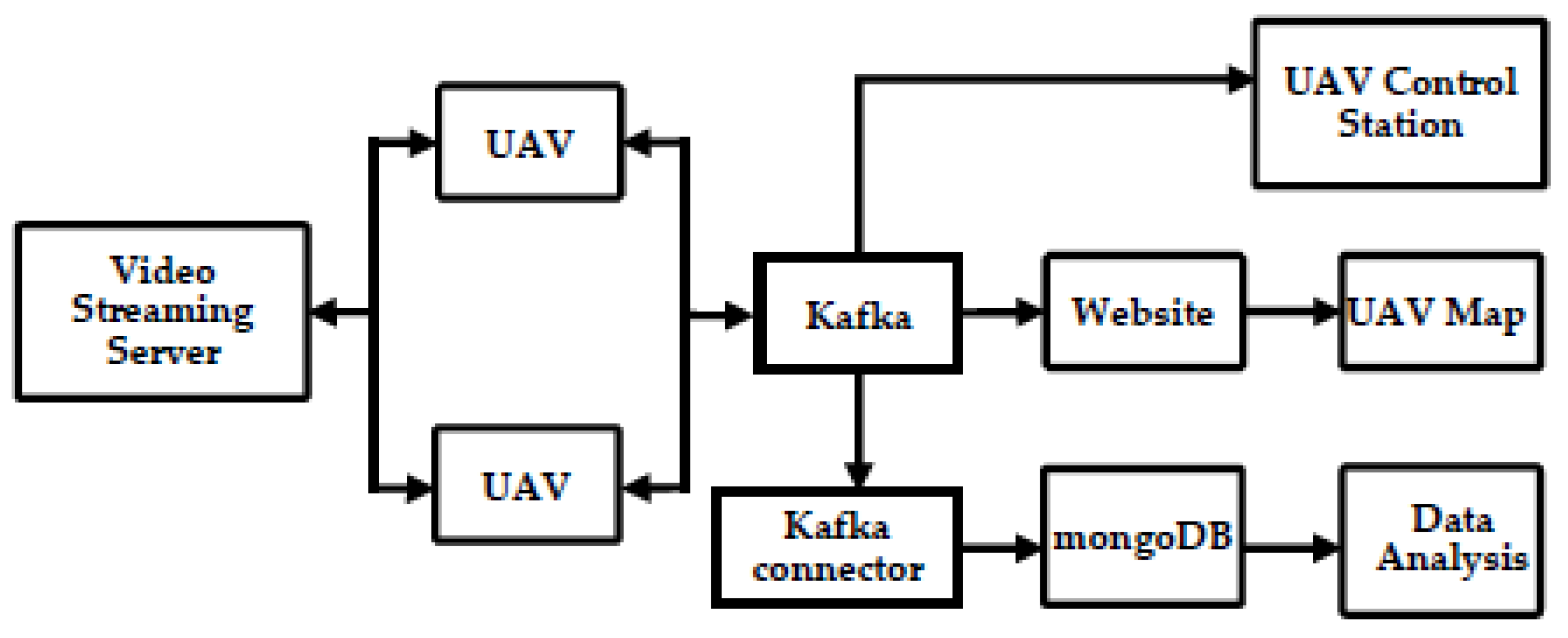
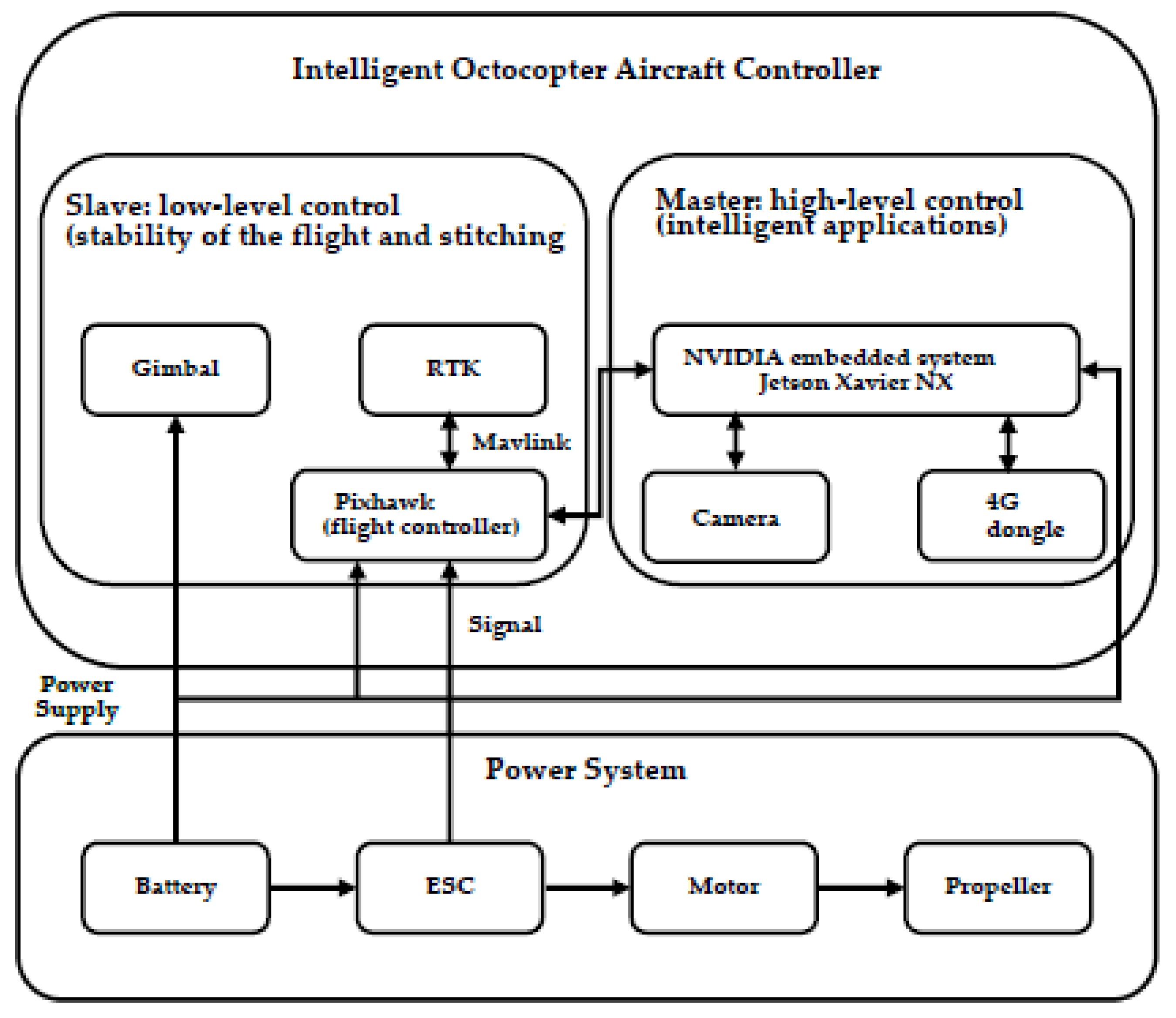
There are ten parts in the real-time UAV riverine waste monitoring system, as shown in Figure 1. The UAV systems are divided into the quadcopter aircraft controller, octocopter aircraft controller, and power system. The intelligent quadcopter and octocopter aircraft controllers utilize Pixhawk [15] to achieve flight stability. The intelligent octocopter aircraft controller assembles the gimbal to achieve image stitching stability and uses real-time kinematic positioning (RTK) to achieve precise positioning. The power system supplies the power to the UAVs and gimbal. Figure 2 shows the architecture of the octocopter aircraft system.
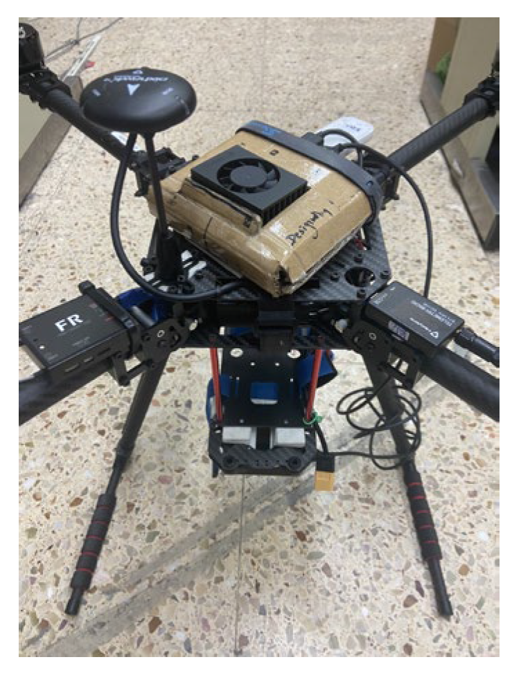
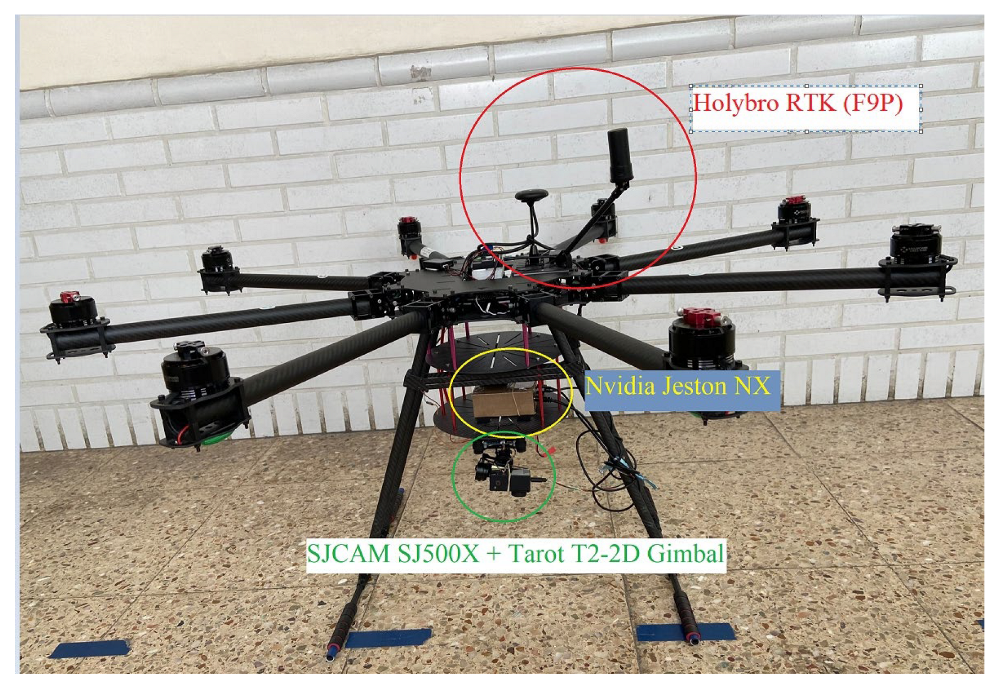
The slave of the octocopter aircraft controller assembles an extra gimbal to achieve high-quality images and replaces the global positioning system (GPS) module with RTK to achieve precise positioning. The masters of the quadcopter and octocopter aircraft controllers perform high-level control, including detecting riverine waste and sending flight commands to the slave. The quadcopter (Figure 3) and the octocopter (Figure 4) aircraft controllers utilize the Pixhawk flight controller. The quadcopter aircraft controller is equipped with the Ublox M8N GPS [16] module to achieve flight stability. In contrast, the octocopter aircraft controller is equipped with the Holybro F9P RTK [17] module to achieve higher flight stability and precise positioning. The position error of the Holybro F9P RTK module is 0.3 m, and the error of the Ublox M8N GPS module is about 3 to 5 m. The PID controller of the quadcopter and the octocopter aircraft are auto-tuned. The limitation of the wind force scale for the proposed UAV system is 4. The maximum wind speed that the UAV can be operated is 8 m/s.
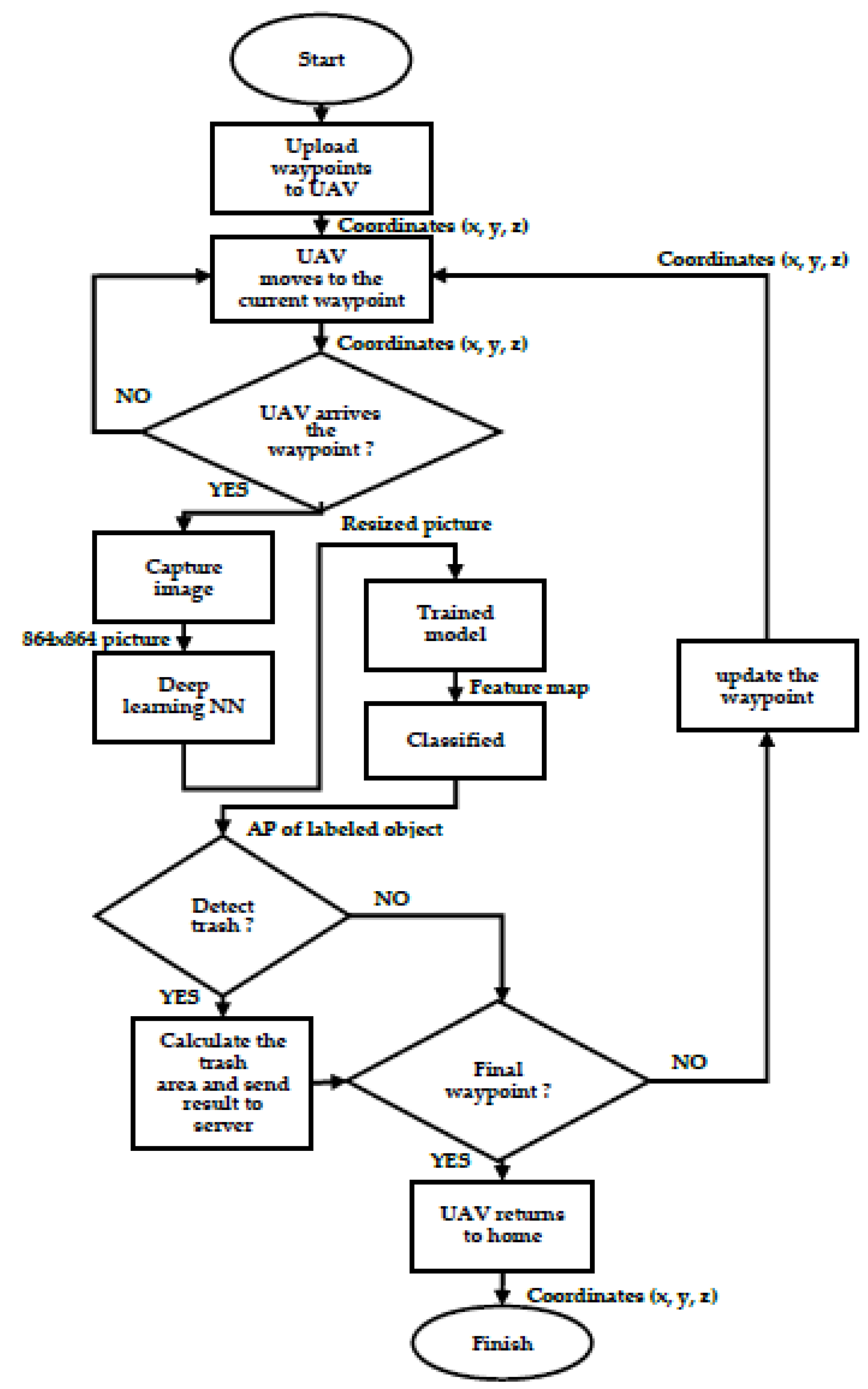
The quadcopter and octocopter aircraft controllers are equipped with the embedded NVIDIA system Jetson Xavier NX [18] as the UAV onboard computers, that can perform high-level computational detection. This study needs to make the UAV system perform image processing, control, and monitoring of various information of the UAV that requires many calculations. The NVIDIA Jetson Xavier NX has many advantages, including its small size, being lightweight, and fast computing speed, and can provide up to 21 trillion operations, achieving excellent performance in real-time computation. Combined with peripheral equipment, drone automation can be realized. The quadcopter and octocopter aircraft controllers are equipped with the SJCAM 5000x [19] webcam and the Huawei E8372 4G dongle [20], respectively. The webcam is attached to the Tarot T2-2D gimbal [21]. The camera’s field of view (FOV) is 120°, and the frames per second (FPS) of 1080 p video is 60. The camera has built-in Wi-Fi and anti-shake digital stabilization, and the ground sample distance (GSD) is 2 mm/px at a 5 m height. For the UAVs’ riverine waste detection mission, we need to measure the coordinates and set the waypoints for the UAVs in advance. Consequently, the UAVs can detect the riverine waste along the riverbank. Figure 5 shows the flowchart of a UAV’s waste detection process. A preplanned path with waypoint coordinates is uploaded to the UAV onboard computer. The UAV flies to the waypoint and captures an image. The image is then sent to the deep learning neural networks for object identification. The classified image with labels is checked by its AP value. If there is garbage, the trash area is calculated and the result is sent to the ground control center. Finally, the UAV’s position is checked; if it is the ending point, the mission is accomplished; otherwise, it moves to the next waypoint and repeats the steps until it reaches the ending position.
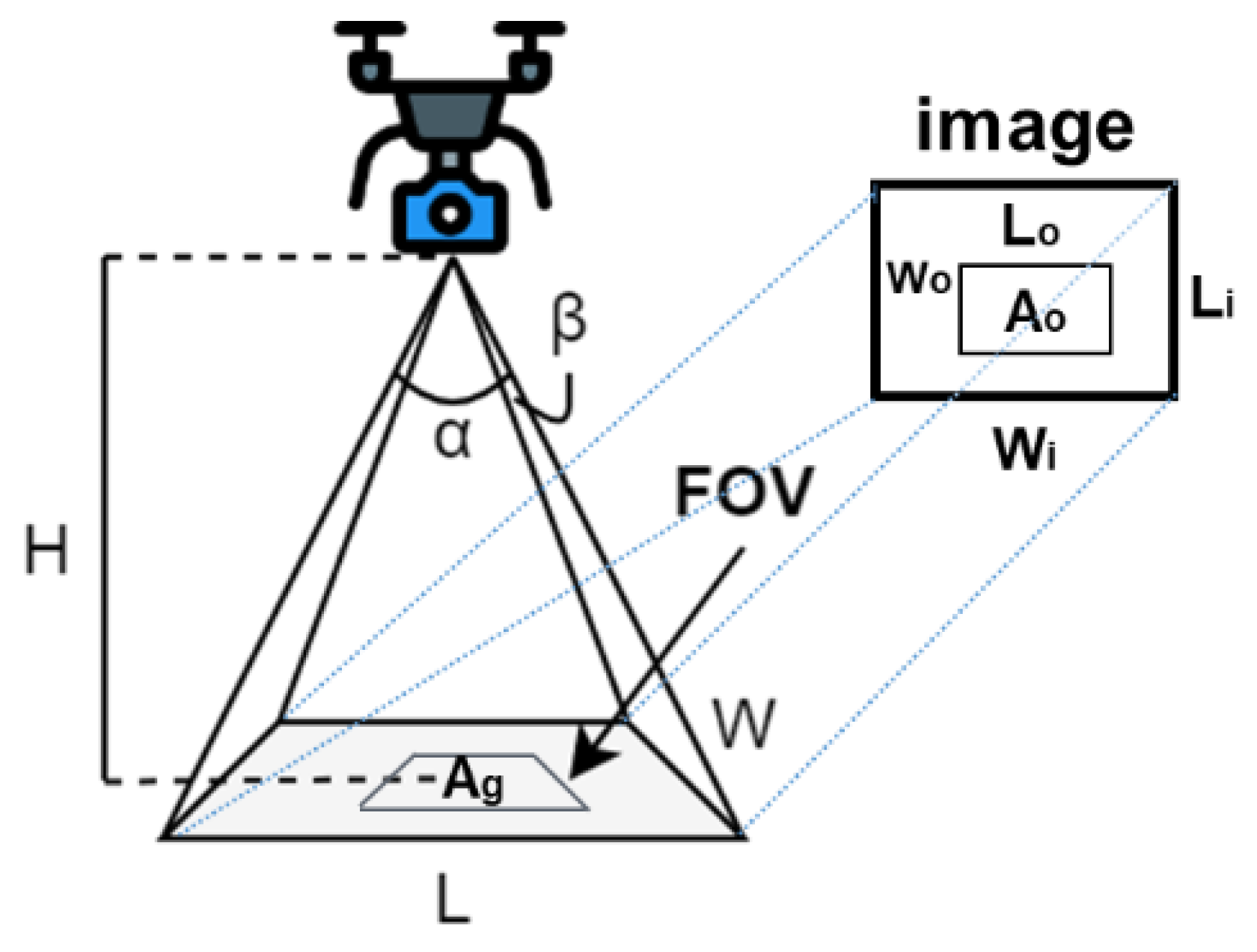
For the UAVs’ dynamic image stitching mission, we set the UAVs’ flight speed to 1 m/s; the UAVs were separated by 4 m. We can calculate the riverine waste pollution area using Equations (1) to (4), where are the camera’s horizontal and vertical angle of view; H is the UAV’s height; L and W are the lengths of the camera’s horizontal and vertical view; Wi and Li are the width and height of the camera’s image; and Wo and Lo are the width and height of the detected riverine waste in the picture, respectively; Ao is the detected riverine waste’s area in the image; and Ag is the area of the detected riverine waste in the real world, as shown in Figure 6.
In the riverine waste monitoring system, the detector detects the riverine waste and calculates the riverine waste pollution area; then, the image is transmitted to the server. This process produces several streaming data. Therefore, we need to set up a suitable information-fusing system for streaming, analyzing, and storing data. Four methods are integrated to build a compelling message queuing system: file transfer, shared database, remote procedure invocation, and messaging. The file transfer is performed through the processor to monitor a folder; if the source produces a file in a folder, the processor captures this file from that folder. Given that the file transfer method has high latency, the file transfer method does not fit our information-fusing system. In the shared database method, applications can use the exact synchronized storage location concurrently. The shared database performs poorly due to the difficulty in defining the boundaries between the same data. For the remote procedure invocation method, a client addresses the demand while the server replies. The disadvantage of this procedure lies in all applications being coupled and the difficulty in integration. The messaging method is asynchronous, which can deal with tightly coupled applications. In this method, the transmitter does not need to wait for a receiver. Further, an application can be developed efficiently in a real-time riverine waste inspection system.
There are several message queuing (MQ) systems, such as Kafka [22], RabbitMQ [23], RocketMQ [24], ActiveMQ [25], and Pulsar [26]. In [27], the authors compared the performance of these systems and tested the throughput in three scenarios, including the numbers of partitions, producers and consumers, and message size. The throughput refers to the number of bytes per time transmitted through the queueing system. Kafka achieved the highest throughput among these queuing systems. Therefore, we selected Kafka as the message queuing system and utilized a Kafka broker to deal with messages from the UAVs. The UAVs’ flight data stream is collected; each UAV produces one partition with one replica. Riverine waste data—detected by the UAVs—is collected, and all the UAVs send the data to the same partition. The UAVs’ real-time maps consume the collected data to monitor the status of each UAV and the area polluted by the riverine waste. The Kafka configuration in the UAV riverine waste monitoring system can be found in our previous work [5].
In different operating systems, a web service is the best way to exchange data between applications. Therefore, we utilized the Python 3.10 web framework Django [28], using the hypertext transfer protocol in the UAVs’ riverine waste inspection system to develop a website running on a computer to facilitate client queries. A real-time UAV riverine waste map was created using a JavaScript library Leaflet [29] for interactive maps with the Django website and Kafka broker to develop a riverine waste pollution monitoring system. Consumers can access information from Kafka via the web service. The riverine waste data (e.g., the position of the UAVs and the area of the riverine waste, which the UAVs obtain) are shown in the riverine waste map.
In the design of the video streaming server, the UAV utilizes 4G communication to transmit the video stream to the server and then release it. Multiple users can subscribe to a video streaming server at 30 FPS (frames per second) through a website. The UAVs first fly to the waypoint and subsequently use the onboard camera’s current altitude and FOV (field of view) to calculate where the UAVs should detect garbage and avoid double detection. Finally, the UAVs send the image back to the server. In addition, the UAVs continuously send real-time video streams to the server while the server simultaneously receives images from the drone’s camera and stitches them together. ZeroMQ [30] is a socket-based concurrency framework featuring intra-process, inter-process, and transmission control protocol (TCP) communication. On the other hand, ImageZMQ [31] is a Python application programming interface (API) for video streaming built on top of the ZeroMQ framework. We leverage the ImageZMQ API with automatic image resizing methods, an automatic reconnection mechanism, and JPEG compression [32] to adapt to varying network conditions.
In the automatic reconnection mechanism, we set the timeout to 1.8 s. This value is determined by trial and error, depending on the network conditions of the server and the UAVs. The UAVs will automatically reconnect to the video streaming server if the disconnection time exceeds the timeout. Through trial and error, the UAVs record the number of timeouts that occur and use this to automatically resize the appropriate image size, with more timeouts resulting in a smaller image size, before sending the video stream to the server. In the waste detection mission, the UAVs continuously receive messages from Kafka topics to check for commands from the control station. Each UAV uses a partition in the topic. If the UAV encounters an emergency, we can issue commands through the UAV control station, allowing the UAV to perform landing or RTL or other actions.
In [33], a performance comparison of seven databases, three SQL (Oracle, MySQL, MsSQL) and four NoSQL (Mongo, Redis, GraphQL, Cassandra), was performed. In experiments, NoSQL databases are faster than SQL databases, among which Mongo performs best. Therefore, we selected Mongo as our database for its excellent performance and schema-free data storage. In Mongo, a collection is created to store the documents. The trash document sent by the UAV contains the identity of the UAV, the time that riverine waste is detected, the latitude position of the riverine litter, and the area of the riverine waste. We used Kafka as the data streaming platform in the waste monitoring system. It must be noted that the data must be accessed and stored in the database. Further, we built the Kafka connector that consumes the data with batch processing from Kafka and transfers the data into the database. The Kafka configuration in the UAV riverine waste monitoring system can be found in our previous work [5].
3. Image Classification
There are a variety of algorithms for image classification, including the backpropagation neural network (BPNN) [34], support vector machine (SVM) [35], and Hopfield neural network [36]. In 2012, an extensive deep convolutional neural network (CNN) called AlexNet [37] showed excellent performance on the ImageNet [38] large-scale visual recognition challenge (ILSVRC), marking the start of the broad use and development of CNN models such as VGGNet [39], GoogLeNet [40], ResNet [41], and DenseNet [42]. In [43], the authors compared the classification accuracy and speed of the four classification algorithms, including k-nearest neighbors (KNN) [44], SVM, BPNN, and CNN. CNN has the best classification accuracy for handwriting digit recognition. In the past few years, deep learning has been proven to be a significantly powerful tool because of its ability to process large amounts of data used for image recognition, video recognition, imagery analysis, and classification. One of the most popular neural networks in image classification is CNN. CNN can design some weights based on the different objects in the image and then distinguish them from each other. CNN requires very little pre-processing of data compared to other deep learning algorithms. The CNN algorithm is based on various steps structured in a specific workflow, including input image, convolutional layer, pooling layer, and fully connected layer for classification.
The convolutional layer is the first layer in the CNN, responsible for the feature extraction of the input images. Convolution is an operation comprising two steps: sliding and inner product. The image obtained after convolution is called a feature map, which uses a filter to slide on the input image and continue to perform the matrix inner product. A pooling layer is usually applied after a convolutional layer, and is responsible for reducing the size of the convolved feature map to reduce computational expense. There are three types of pooling: average pooling, max pooling, and sum pooling. We mainly utilized max pooling, where the filter selects the largest element from the region of the feature map. After extracting features and reducing the image parameters from the convolution layer and max pooling, the feature information will be passed to the fully connected layer. The fully connected layers in a neural network are those where all the inputs from one layer are connected to every activation unit of the next layer; each connection has its own independent and different weight. Consequently, it will result in the fully connected layer taking in a variety of computations.
3.1. Image Recognition Algorithm
In recent years, artificial intelligence has been applied to many tasks. Object detection is also the most popular part of deep learning. It can be used in various aspects, such as license plate recognition, autonomous driving, product defect detection, and medical image recognition. There are many tasks related to image recognition. Accordingly, the target detection framework is divided into two-stage and one-stage methods.
- Two-stage: In object detection, the general method involves first selecting objects; the process of selecting objects is called region proposal. The chosen objects’ sizes may differ, so the object detection may only be classified or include feature extraction and classification. The two-stage method needs to find the region proposal first before performing detection. The classic two-stage method is the faster region-based convolutional neural network (Fast R-CNN).
- One-stage: A common problem with the two-stage method is that too many objects are selected for real-time computing. The one-stage method operates the object position detection and recognition in one step. The neural network can detect the object’s position and recognize the object simultaneously. While the one-stage method is faster than the two-stage method, its recognition accuracy is not on a par with the latter. Recognition accuracy is still within an acceptable range in the one-stage method. Therefore, the one-stage method is currently more developed and used on mobile devices. The classic one-stage methods are YOLO and single-shot detector (SSD).
In this study, we selected the YOLO algorithm as the waste detecting algorithm. In July 2021, YOLOR-D6 ranked first in the real-time object detection benchmark on the common objects in context (COCO) dataset. A better tradeoff can be found based on speed and accuracy [45]. In YOLOv4 [46], the authors proposed two neural networks, named cross-stage partial (CSP) Darknet53 and CSPResNeXt50, as a backbone to operate quickly and compute optimizations in parallel. The authors found that the CSPResNeXt50 is suitable for classification, while the CSPDarknet53 is suitable for object detection. In YOLOv4, the authors proposed the path aggregation network (PANet) and spatial pyramid pooling (SPP) as the neck instead of the feature pyramid network (FPN). The PANet is modified by the FPN, which adds one more layer that can accurately store spatial information. It can correctly locate pixel points and form masks. On the other hand, there are more channels where the amount of calculations will increase. The SPP extracts features and connects them for deeper depth features.
In [47], the authors compared various activation functions, including rectified linear unit (ReLU), swish, and mish. The mish activation function outperforms all the other activations. Mish is bounded below and unbounded above; its range is in . It avoids saturation, which generally causes training to slow down drastically due to near-zero gradients, resulting in strong regulation effects and reduced overfitting.
The intersection over union (IoU) loss [48] was proposed for the bounding box regression loss function in 2016. The authors proposed GIoU loss [49] in 2019, and DIoU loss [50] and CIoU loss [51] in 2020. The CIoU loss considers the overlap area, point distance, and aspect ratio, making its convergence accuracy higher than GIoU. In GIoU, the DIoU can be used instead of IoU in the NMS algorithm, which is DIoU-NMS. The NMS has four bounding boxes, and the DIoU-NMS has five in the same scenario. Therefore, the authors utilized CIoU loss and DIoU-NMS in YOLOv4. The formula for DIoU-NMS is shown in Equation (6). is the classification confidence, is the threshold of the DIoU-NMS, and M is the bounding box with the highest confidence. Compared to the IoU loss, GIoU loss, DIoU loss, CIoU loss, and CIoU loss, the DIoU—NMS in YOLOv3, CIoU loss with the DIoU—NMS can improve the average precision.
YOLOV4-tiny [46] is the compressed version of YOLOv4. The CSPOSANet is modified by CSPNet and VoVNet [52]. VoVNet consists of a one-shot aggregation (OSA) module that aggregates all the layers before the last layer. In YOLOv4-tiny, the network structure is less complicated than in YOLOv4, and the parameters are reduced so that the training and detection are faster than in YOLOv4. The inference time in YOLOv4-tiny can reach 371 FPS (frames per second). On the other hand, YOLOv4-tiny-3l utilizes three YOLO heads to detect large objects, medium objects, and small objects. YOLOv4-tiny-3l can reach a higher accuracy and precision than YOLOv4-tiny on the COCO dataset.
In 2021, the BottleneckCSP module was proposed to extract the features on the feature maps in YOLOv5 [53]. It can reduce the repetition of gradient information in the optimization process of CNNs. The authors of [53] adjusted the width and depth of BottleneckCSP and developed four models called YOLOv5s, YOLOv5m, YOLOv5L, and YOLOv5x. YOLOv5s has the smallest size and model parameters of the four structures. Conversely, YOLOv5x has the biggest size and model parameters of the four structures. The focus module was proposed, which slices the image before the image input enters the backbone. It can extract four times as many features as without the focus module in exchange for four times the amount of computation. For example, our input image size is 864 × 864 × 3; using the focus module, the output size becomes 432 × 432 × 12, as shown in Figure 7. Comparison of the modern YOLO includes YOLOv3, YOLOv4, and YOLOv5. Regarding average precision, YOLOv4 achieves the best performance on the COCO dataset in the experiment. In terms of inference time, YOLOv5s is better than YOLOv4. When the batch size is adjusted to 36, the inference time can reach 140 FPS.
3.2. Dataset
We need to collect data in advance to train the model for riverine waste detection. In data mining, we utilize the TACO dataset, drinking waste classification dataset, TrashNet, HAIDA trash dataset, and the images collected by the UAVs. We collected 2595 images and divided them into one class (11,318 garbage objects) and 876 negative samples. We also split the data into two categories (7488 garbage objects and 3830 bottle objects) for classification. The data we used and collected is called the riverine waste dataset. The TACO dataset is a dataset of waste from beaches and streets, but the trash is small. The drinking waste classification dataset is full of drinking waste and is divided into four classes (cans, plastic bottles, glass bottles, and milk bottles). We utilized TrashNet, which comprises 2527 images and is divided into six categories (glass, paper, cardboard, plastic, metal, and trash). UAVs collected the HAIDA trash dataset at different heights, and the data are divided into two classes (garbage and bottles). We also downloaded some riverine waste images from the internet, no matter whether the waste was large or small. Most of the data were taken from different places such as Kibera, Indonesia, Manila, etc. We also collected riverine waste images using UAVs; negative samples were also collected.
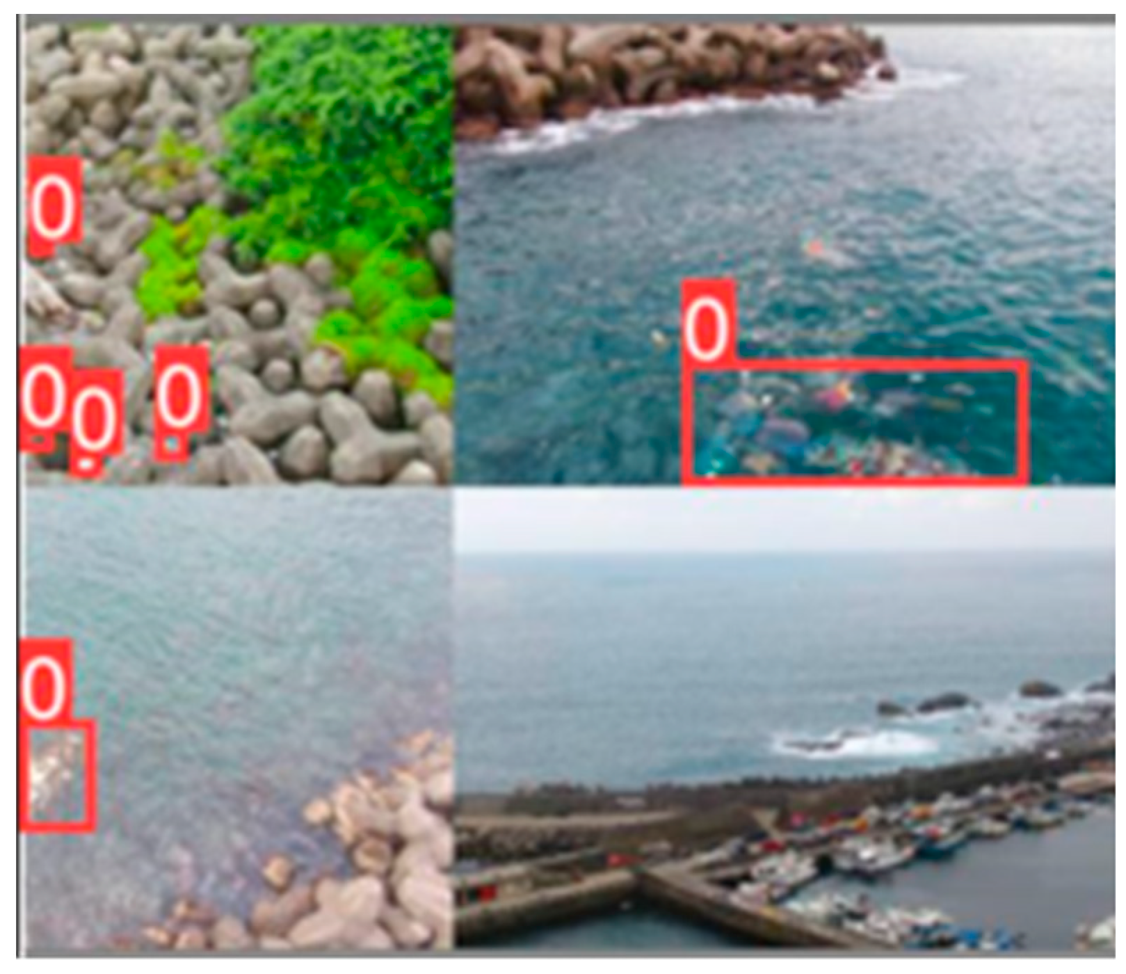
Data augmentation is a method that increases the amount of data. Many data augmentation algorithms have been proposed, such as mixup [54], cutmix [55], cutout [56], mosaic [46], attentive cutmix [57], random erasing [58], dropout [59], and DropBlock [59]. The first data augmentation method used for YOLOv4 is mosaic. The mosaic data augmentation method merges four images into one. This method allows the mode to learn how to recognize smaller objects and increase batch size in training, as shown in Figure 8. The bounding boxes in Figure 8 are the objects to be learned by the neural networks.
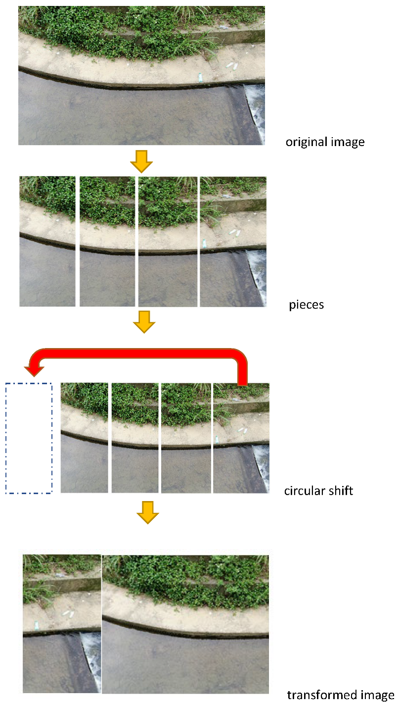
The circular shift method [7] cuts the original image proportionally, shifts the last image to the first position, and transforms all the images into a new one. With different networks, including VGG16, ResNet, SqueezeNet, and DenseNet, utilizing the original and circular shift datasets can achieve higher performance in VGG16, ResNet, and DenseNet. The operation steps include the original dataset, circular shift, and the combination of crop, rotation, and flip. These steps will repeat until the image transforms into the original image, as shown in Figure 9.
Regularization is used to reduce the error and over-complexity of machine learning, commonly known as generalization error. In the training process, the model produces many parameters that may cause overfitting. Therefore, there are various regularization methods to avoid model overfitting and help the model reduce the parameters to promote generalization. Regularization methods include dropout, DropBlock, L1 regularization [60], and L2 regularization [61]. In the model we trained, if the model has too many parameters and too few training data, it is easy for the model to have overfitting. Therefore, dropout can ignore a feature randomly to reduce the parameters that can make the model utilize its generalization. It only depends a little on some local features, bringing out overfitting. The DropBlock method is a form of structured dropout where the features in a contiguous region of the feature map are dropped together. Dropout is widely utilized in fully connected layers and performs well. However, it is not suitable for convolutional layers because the features are spatially related to each other. DropBlock can address the features being spatially associated with each other and reduce the dependence on features.
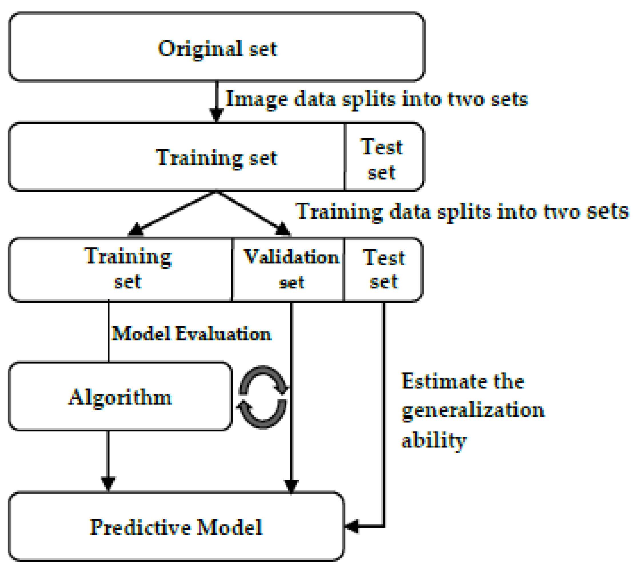
After collecting the data, we need to evaluate the model and verify the generalization ability of the model to independent test data. If we reuse the test set, which means the test set is part of the training set, it can easily lead to overfitting. Several methods can be used to split the data and verify the model, including the hold-out method [62], k-fold cross-validation, nested k-fold cross-validation, repeated k-fold validation, stratified k-fold validation, and group k-fold validation [63]. The hold-out method splits the dataset into training and test sets, and the training set splits again and produces a validation set. The training set is used to fit the different models, while the validation set is used for the model evaluation. The test set is used for estimating the generalization ability of the model. A diagram of the hold-out method is shown in Figure 10.
The k-fold cross-validation method splits the data into k equal parts, meaning the same model is trained k times. The k-1 fold is the training set for the training, and the remaining fold is used for validation. Finally, the loss of the k times is summed up and averaged, which is considered the final result. The nested k-fold cross-validation method is modified by k-fold cross-validation and is divided into two parts: the outer loop and the inner loop. The inner loop tunes the hyperparameters and chooses the best parameters. Then, the model is trained with the best hyperparameters, and the generalization ability is estimated in the outer loop. Repeated k-fold cross-validation means to repeat n times. Every time it is repeated, it splits the data. Then, the k-fold cross-validation is performed, and the best performance is selected. Each fold is split in proportion to the category. In this study, we divided the data into two classes. The proportion is about 1:2, so the ratio of the two classes in each fold must also be 1:2. This method, useful for unbalanced data, is modified from the stratified k-fold cross-validation method. It prevents continuous data from resulting in overfitting. When the data are split in this method, it selects each block from the data and is randomly set as validation. The cross-validation methods are accurate and can prevent model overfitting. On the other hand, the computation time is more than for the hold-out method. Compared to the methods we mentioned, the hold-out method has a simple way to split the data and prevent model overfitting. In this study, the training set accounts for 70 percent of the collected data, the validation set accounts for 20 percent, and the test set accounts for 10 percent.
3.3. Training
There are several learning rate decay methods, including poly, random, and steps. The poly method adjusts the learning rate with every training step, as shown in Equation (7). The random method gives the learning rate randomly for every training step, as shown in Equation (8). The steps method decays the learning at specified steps. For example, we set the specified step to 8000 and 9000, the decay ratio as 0.01, and the initial learning rate as 0.05. In the step set at 8000, the learning rate was adjusted to 0.005, while in the step at 9000, the learning rate was adjusted to 0.0005.
A comparison of the state-of-the-art (SOTA) object detection algorithms is shown in Table 1. This study focuses on FPS and AP50 (Val). The YOLOv4-tiny-3l model can achieve 75.4% AP50 (Val). This performance is the best in this model, and its inference time of 175 FPS is good. YOLOv5m reaches 74.4% AP50 (Val), close to YOLOv5s. However, its inference time is lower than YOLOv5s. Hence, this study compared the performance of YOLOv4-tiny-3l and YOLOv5s on a test set.
The results show that the confidence scores of YOLOv4-tiny-3l are higher than those of YOLOv5s in the same frame, as shown in Figure 11 and Figure 12. While both did not miss trash, only YOLOv4-tiny has false detection, as shown in Figure 13 and Figure 14. Therefore, this study selected YOLOv5s as the riverine waste detection algorithm and proposed improving YOLOv5s for better performance.
For the hyperparameter tuning for YOLOv5s, we adjusted the input size, filter size, iterations, learning rate, activation function, mosaic, learning rate decay, and dropout method. When the input size is 864 × 864, the number of iterations is 13,000, the learning rate is 0.005, and the decay steps are at 8000 and 9000, with the mish activation function and without mosaic data augmentation, the AP50 (Val) can reach 78.2%. If we add a dropout layer in YOLOV5s, when we use DropBlock and cover 50% of the features, the AP50 (Val) drops to 74.5%. If it covers 30% of the features, the AP50 (Val) is 76.2%, as shown in Table 2.
After tuning the hyperparameters, we modified the structure of YOLOv5s to achieve a higher performance in detecting riverine waste. Therefore, we proposed the improved YOLOv5s-i, improved YOLOv5s-ii, and improved YOLOv5s-iii. The improved YOLOv5s-i adds eleven additional convolutional layers in the neck, including four filters for 32 convolutional layers, six for 64 convolutional layers, and one for 128 convolutional layers. The AP50 (Val) improves by 78.6% in the improved YOLOv5s-I. Improved YOLOv5s-ii adds fifteen additional convolutional layers in the neck, including four filters for 32 convolutional layers, ten for 64 convolutional layers, and one for 128 convolutional layers. The AP50 (Val) improves by 79.3% in the improved YOLOv5s-ii. Improved YOLOv5-iii adds 22 additional layers in the neck, including five filters for 32 convolutional layers, fifteen for 64 convolutional layers, and two for 128 convolutional layers. The AP50 (Val) improves by 79.6% in the improved YOLOv5s-iii. Based on the improved YOLOv5s-ii and improved YOLOv5s-iii, we found that adding more layers did not significantly improve the AP50 (Val). To verify this conjecture, we added 27 additional layers in the neck, including five filters with 32 convolutional layers, fifteen filters with 64 convolutional layers, and four filters with 128 convolutional layers. The AP50 (Val) drops to 78.1%.
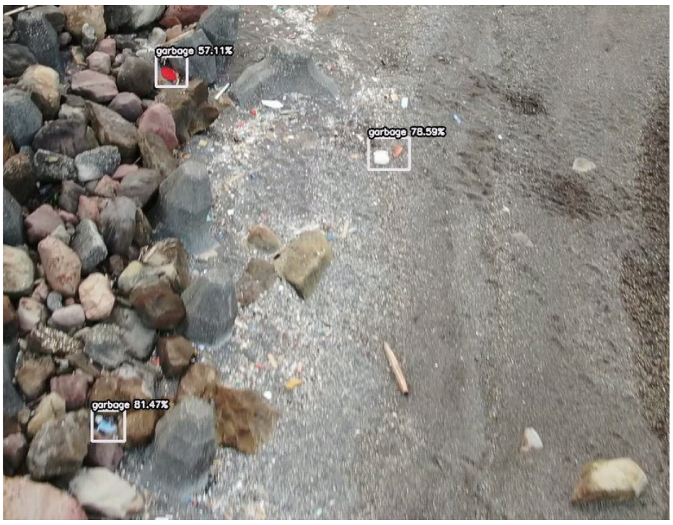
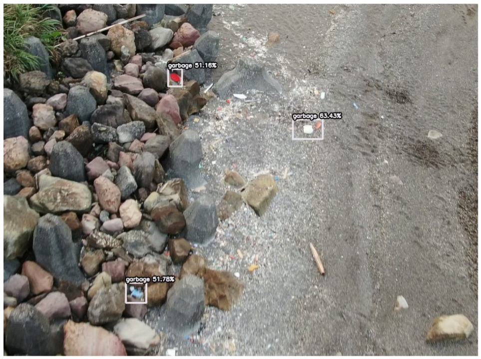
Finally, the improved YOLOv5s-iii was selected as the riverine waste detection algorithm. The hold-out method was used to split the riverine waste dataset first. It split the data into 70% for the training set, 20% for validation, and 10% for the test set. We used a test set to verify the proposed structure. Notably, the improved YOLOv5s-iii performed well. The confidence scores of the improved YOLOv5s-iii increased by 20% in the test set, as shown in Figure 15.
4. Image Stitching
Image stitching is performed when images have overlapping areas. Image stitching methods can be classified into region-based and feature-based image stitching.
- Region-based image stitching: This method is divided into two parts. One part of the region-based image stitching method is applied in the space domain, and the other is in the frequency domain. In the space domain, the method is used to select an area in the overlapping areas as a template and search for the blocks of another image. The most relevant areas are the matching areas. In the frequency domain, images are transformed by discrete Fourier transform. Then, the correlation function of the space domain is obtained by inverse Fourier transform, and the best matching areas to the correlation function are calculated.
- Feature-based image stitching: This method finds the features in the scale space by the extrema value detection and then positions the features. The feature description obtains the matching areas and stitches the images. Feature-based image stitching is a commonly utilized method because its computational cost is lower than the region-based image stitching method. Therefore, several algorithms have been proposed, including the SIFT, SURF, and ORB.
In [64], the authors compared the three methods: SIFT, SURF, and ORB. According to their tests, the stitching results of the three methods are similar. The most significant difference lies in the computation: the SIFT algorithm takes the most computing time because it extracts the most features. On the other hand, the ORB algorithm takes the least amount of computing time. In this study, the SIFT algorithm is used as the image stitching method. Although the SIFT algorithm spends more computing time for stitching, it can extract more features to stitch images, and the computing time is acceptable for the proposed system. There are four steps for feature detection in SIFT [13], including the extrema value detection in scale space, keypoint localization, orientation assignment, and keypoint description. An image in scale space is similar to the image people see in the real world but is in the computer vision space. It presents far, near, clear, and blurred images using the Laplace of Gaussian (LoG) function. In scale space, the difference of Gaussian (DoG) function is used for determining the extrema value. Equation (9) is the Laplace of Gaussian function, and Equation (10) is the difference of Gaussian function.
After using the difference of Gaussian function to determine the extrema value, the value is not necessarily a true extrema value because it may be a discrete point. Therefore, the Taylor series is used to find a real extrema value, named the keypoint, as shown in Equation (11). It eliminates boundary responses that include low-contrast or poorly positioned points using a Hessian matrix, as shown in Equation (12). The Hessian matrix is used to calculate curvatures, as shown in Equation (13). is the largest value, and is the smallest value. If the curvature is less than ten, the keypoints may be close to the boundary and can be eliminated.
To let the onboard computer obtain these keypoints, we need to provide keypoint orientation, which means converting them to vectors. Equation (14) shows how the gradient values of keypoints is calculated. Equation (15) shows how the orientation of keypoints is calculated.
Before this step, each keypoint can receive three messages, including position (x, y), scale , and orientation . Then, the vectors in eight directions are counted, and the main direction for the keypoint is determined. If several directions differ by less than 20%, the main directions can be more than one direction. When the image is rotated, the main direction is used to correct the right direction; the vectors will not change.
The SURF algorithm is a further optimization of the SIFT algorithm. SURF is faster than SIFT and can achieve real-time implementation of applications. It utilizes a box filter instead of a Laplace of Gaussian filter, which can reduce a significant amount of computation time; hence, SURF is fast. SURF utilizes Hessian matrix determinant approximation instead of the difference of Gaussian function calculation. In addition, it uses box filters to simplify the Gaussian filters. SURF uses Harr wavelet features in the field of counted feature points instead of gradient histograms. In a circle with a radius of 6s, s is the scale of the feature point. The sum of the horizontal Harr wavelet and the vertical Harr wavelet features of all points in the 60-degree sector is calculated. Then, it is rotated at 60 degrees until it turns a circle. Finally, the maximum value is used as the main direction of the feature point. Before this step, each keypoint can receive four messages, including the sum of the horizontal values, the sum of the vertical values, the absolute value of the sum of horizontal values, and the absolute value of the sum of vertical values.
In oriented FAST and rotated Brief (ORB) [65], FAST is used to detect the keypoints, and Brief is used to describe the keypoints—both have good performance and low computation. FAST gives a pixel in an array, compares the brightness of with a circle of 16 pixels around it, and then classifies the pixels into three categories: brighter than , darker than and similar to . If more than eight pixels are brighter or darker than , is selected as a keypoint. The original FAST method cannot have orientation. Therefore, ORB assigns an orientation to each keypoint depending on how the intensity level around the keypoint changes. The Brief descriptor is used to describe the keypoints. It utilizes a bit string, a binary intensity test set that describes the image patch. ORB uses rotation-aware Brief to deal with Brief’s matching; its performance degrades dramatically for rotation beyond a few degrees.
5. Experiments and Results
The parameters used in this study are listed in Table 3 and Table 4. Image stitching is a complex problem when the object is moving, or the scene is changing. The light, image quality, and many factors affect the image stitching result. Therefore, image stitching is divided into static and dynamic scenes.
- Static scene: A static scene does not mean that the scene is not changing. It usually refers to the cameras being sedentary. The background does not move; conventional methods can find moving objects, and camera images can be stitched.
- Dynamic scene: A dynamic scene means that the scene changes constantly, including the background and the objects. It is difficult to stitch images from moving cameras.
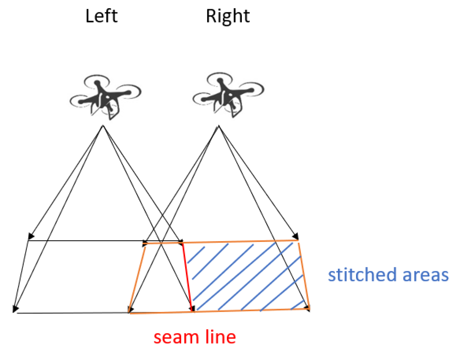
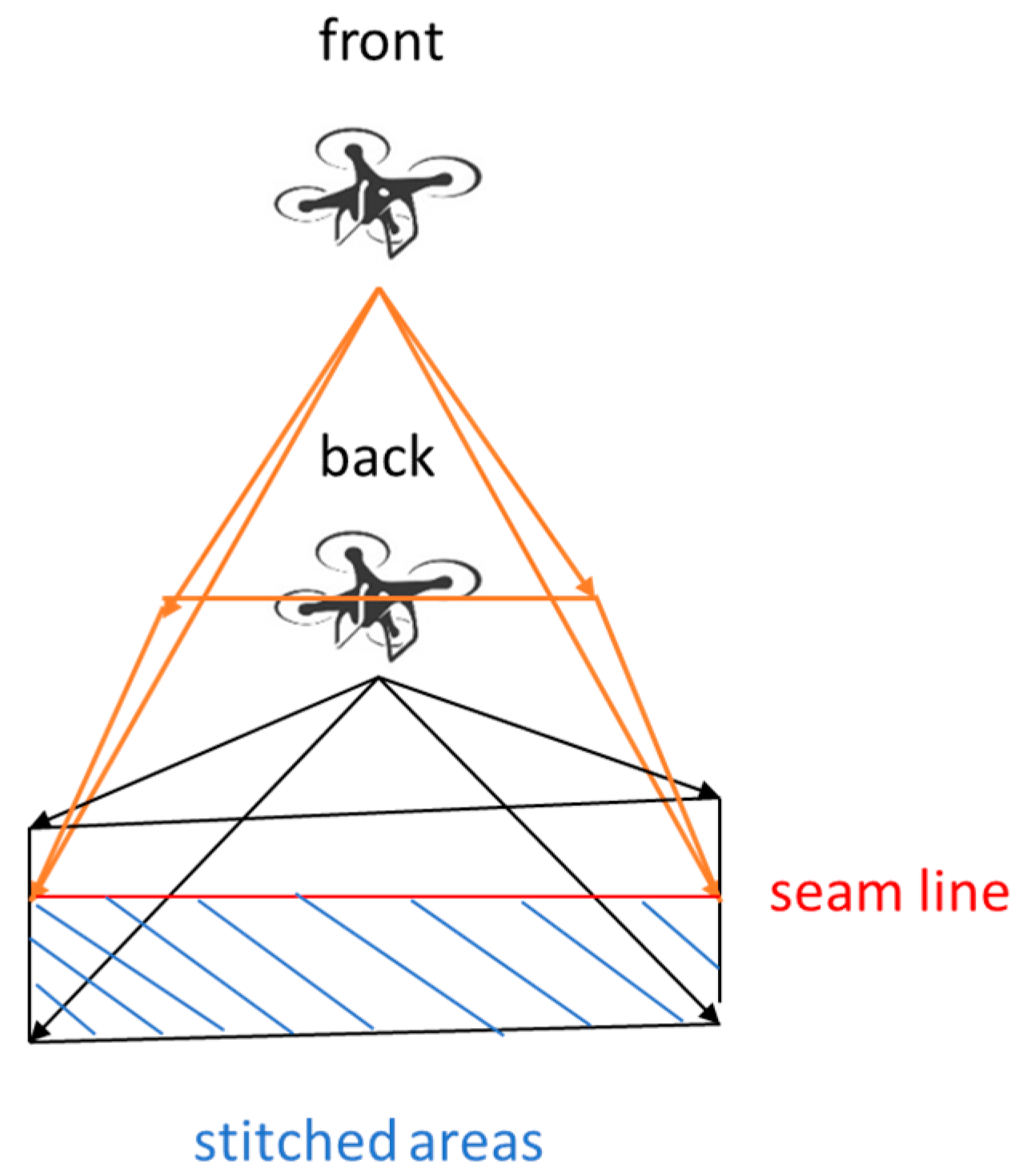
In [66], the authors proposed that on each side of the seam line, only the image from the camera’s image must be selected to address the failure rate and computing time of dynamic scene stitching. For example, if two images are stitched, and the left camera’s image of the right seam line does not move, the right camera’s image is selected for stitching. If the overlapping area is enough, the images can be stitched. Therefore, we selected this stitching method. The image on the left side does not change, and the right side image is used for stitching, as shown in Figure 18. If the cameras’ positions are at the front and back, the front side image does not change, and the back side image is selected for stitching, as shown in Figure 19.
There are three scenes in our test environment: (1) the National Taiwan Ocean University (NTOU) campus; (2) the Tianliao River, based on the Keelung Bureau of Environmental Protection and the Society of Wilderness’s suggestions; and (3) the Keelung River. We utilized the embedded NVIDIA system NX on the UAVs to realize real-time detection and sent the image from the UAVs’ cameras to the ground station server for stitching. In the riverbank inspection mission, if the UAVs encountered an emergency, we could give a command to let the UAVs land, return, or perform other operations through the UAV control station.
5.1. Scene 1: NTOU Campus
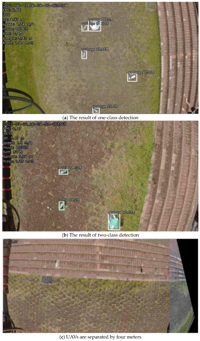
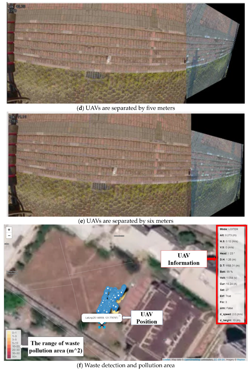
In the riverbank inspection, the waste was divided into one class (garbage) and two classes (garbage and bottle). First, we put some plastic bags and bottles on the campus. We set the UAVs’ height to five meters and speed to 1 m/s. For one-class detection, the confidence scores for garbage detection are high (54.81%, 90.31%, 95.1%, 98%, 98.86%), as shown in Figure 20a. For the two classes, the confidence scores for garbage and bottles are still high (80.03%, 94.12%, 98.2%), as shown in Figure 20b. However, they are slightly lower than the one-class case. In image stitching, UAVs hovered first and then tried to find the maximum distance for effective stitching, as shown in Figure 20c–e. When the distance between the UAVs exceeded six meters and the image overlap area was less than 30%, the stitching results were bad. The real-time detection data and the pollution area were indicated on the ground station monitor, as shown in Figure 20f,g. Each blue dot in Figure 20f is the waypoint of the flight trajectory; it contains the coordinates of the location and garbage information. Detailed information is shown in Figure 20g. After analysis, the waste location is indicated on the heatmap, as shown in Figure 20h. Garbage information can be successfully demonstrated at the ground station (control center). Government officials can check pollution information from the real-time images provided by our riverbank inspection system. The officials can move the cursor by using the computer mouse and pointing at the blue dot on the computer screen. Then, the garbage size and coordinates will appear on the screen, as shown in Figure 20f,g. In addition, the areas of the detected debris are also shown in Figure 20a,b on the left side of the pictures; they are indicated as “trash: 1.47 m2” and “trash: 1.43 m2”, respectively. The proposed system can reduce labor spent on garbage inspection a lot.
5.2. Scene 2: Tianliao River
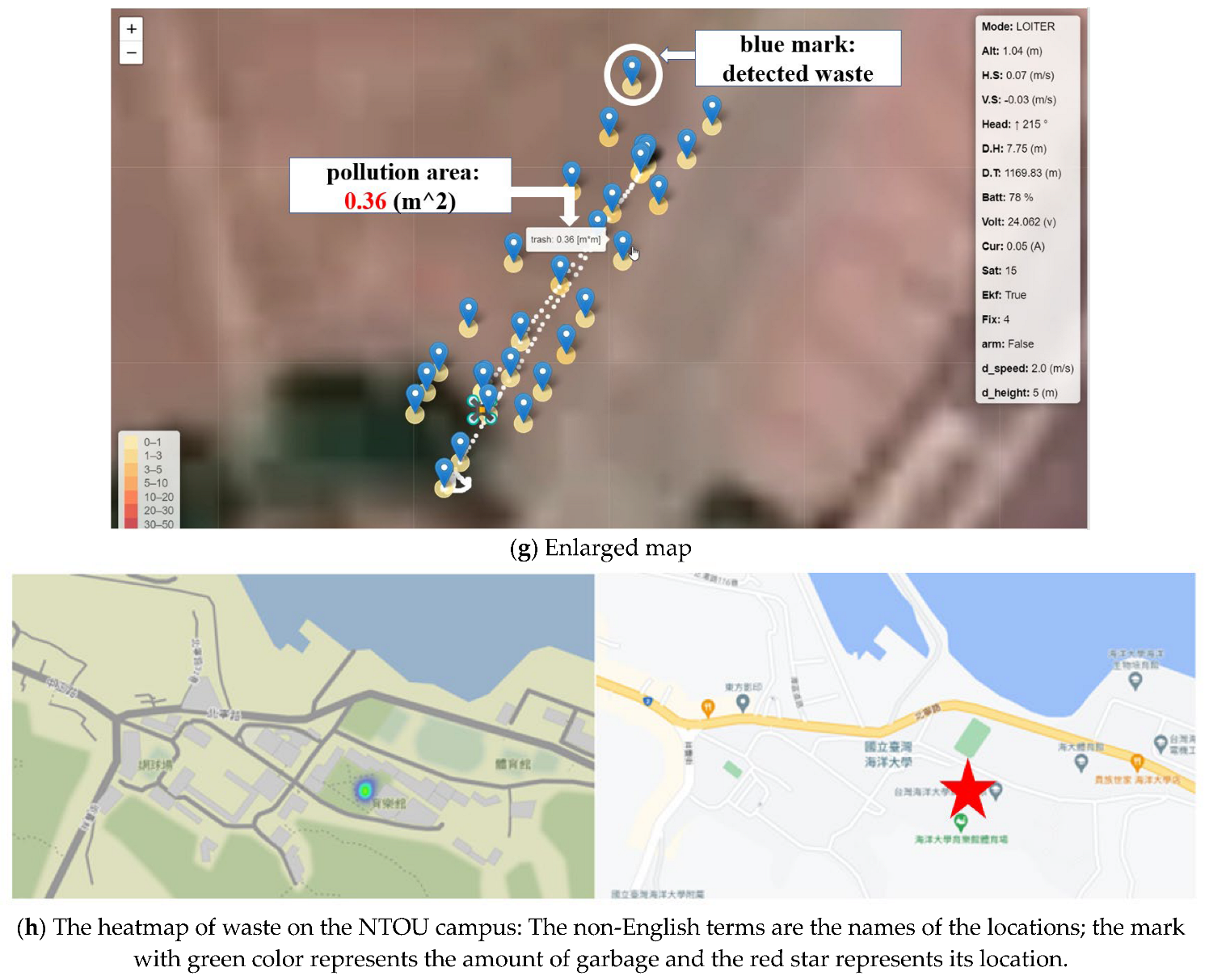
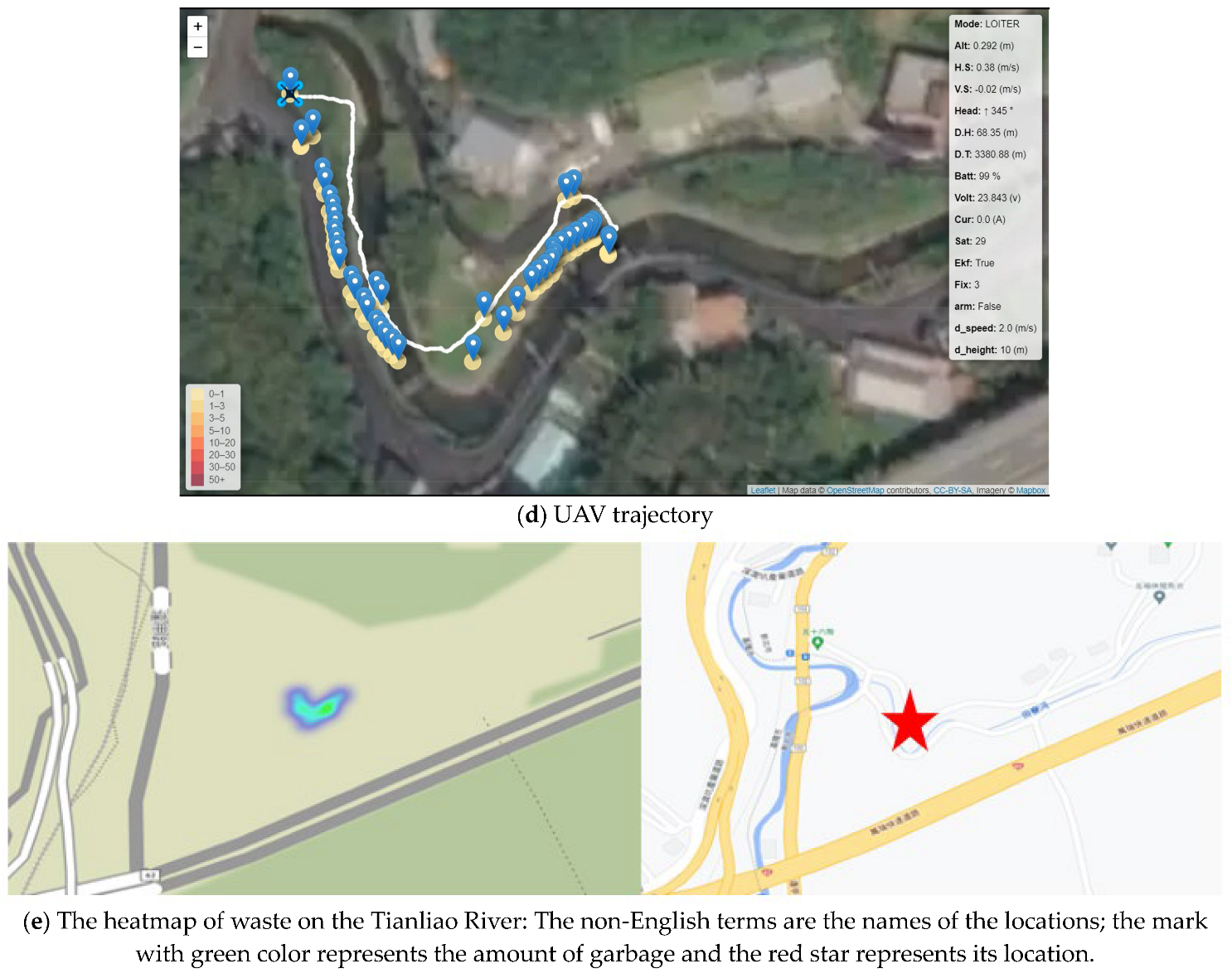
At the Tianliao River, some garbage and bottles are stuck in stones. The UAVs’ height was about 5 m above the riverbank, the speed was about 1 m/s, and UAVs were separated by 4 m. In riverine waste detection, the detector could recognize two classes well when tested in NTOU. Therefore, we only tested two-class detection in the Tianliao River, as shown in Figure 21b, and all garbage was identified. On the day of the test, the wind speed reached 6 m/s to 8 m/s, and the UAVs’ heights differed, making the size of both cameras’ images different. Further, the gimbal and UAVs were unstable due to the strong wind. Although the result is not remarkable, the images could still be stitched, as shown in Figure 21c. The trajectories of the UAVs are shown in Figure 21d; each blue dot represents a location with garbage information on it. The heatmap of waste is shown in Figure 21e. The area of the detected debris is shown in Figure 21b on the left side of the picture; it is indicated as “trash: 0.35 m2”. The confidence rates of the detected debris are shown in Figure 21b (62.04%, 40.51%, 38.47%, 62.34%).
5.3. Scene 3: Keelung River
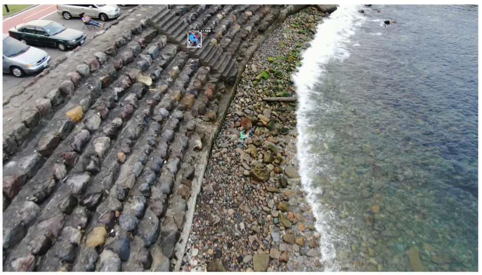
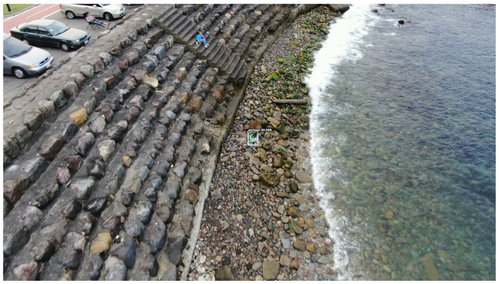
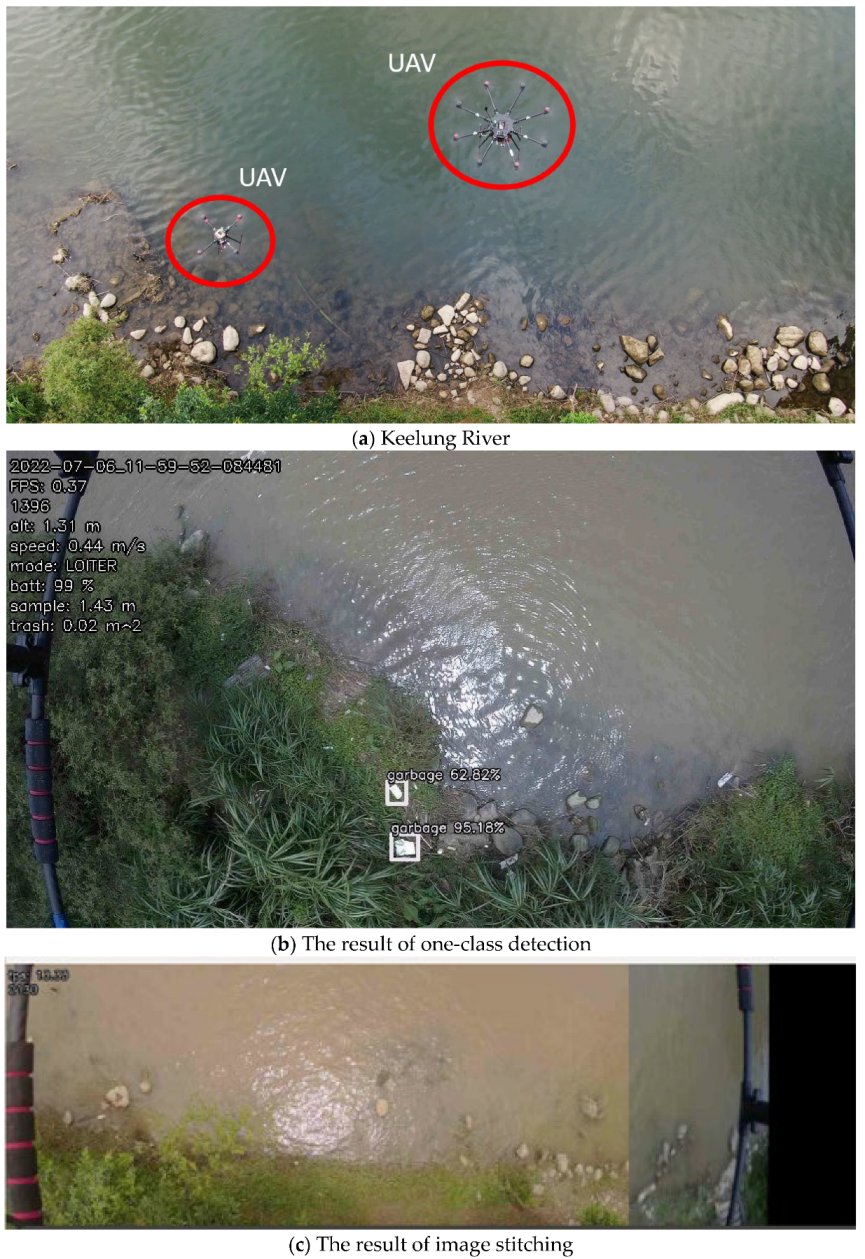
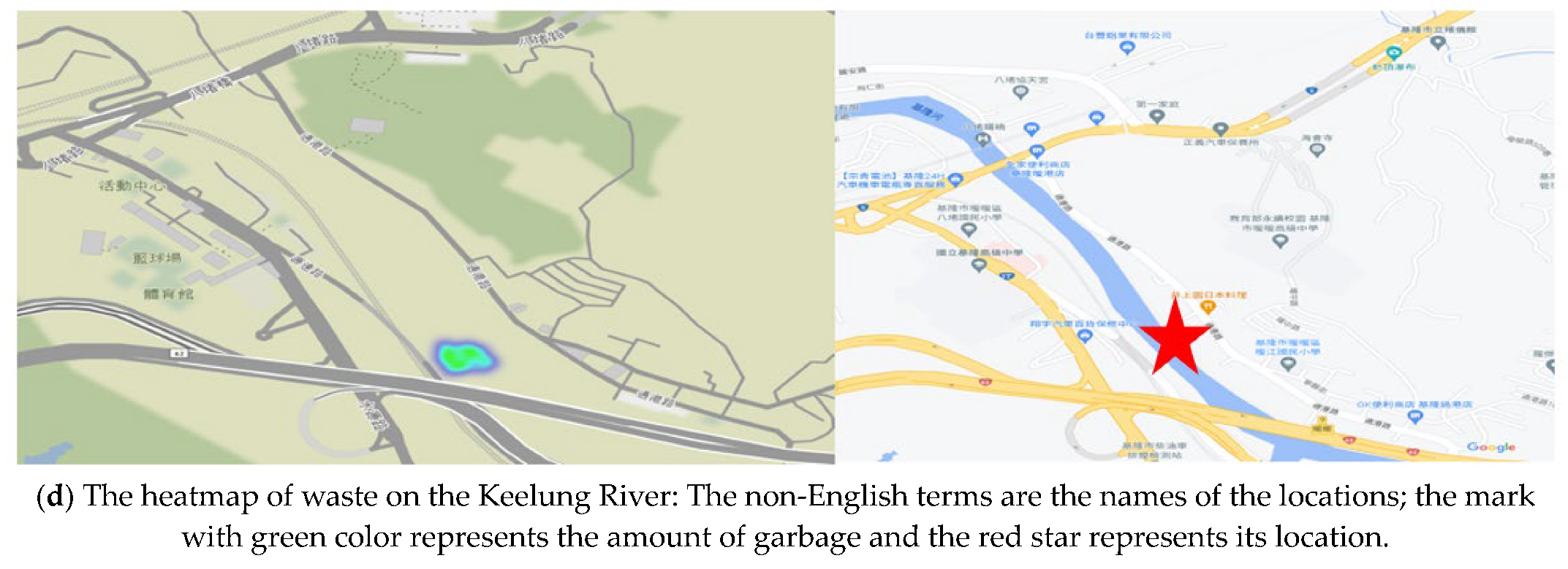
In the Keelung River test, we set the UAVs’ height to about 5 m above the riverbank, the speed was about 1 m/s, and the UAVs were separated by 5 m. In riverine waste detection, some small garbage could be detected. The confidence scores are high, as shown in Figure 22b. For image stitching, we set the UAVs farther away from each other. Images can be stitched, as shown in Figure 22c. The heatmap of waste is shown in Figure 22d. The area of the detected debris is shown in Figure 22b on the left side of the picture; it is indicated as “trash: 0.02 m2”. The confidence rates of the detected debris are shown in Figure 22b (62.83%, 95.18%).
Table 5 demonstrates the effectiveness of the proposed trash inspection system by summarizing the detected results from three different scenes. The experimental results show that if the background of the test field is complex, there are undetected objects. To overcome this problem, more training images are needed. The position accuracy is good in the three scenes. This is because the RTK system is used in the proposed UAV system.
6. Conclusions
In waste detection, we found that the improved YOLOv5s-iii is better than YOLOv5s and YOLOv4-tiny-3l after tuning the hyperparameters and modifying the YOLOv5s model. When we tested it on rivers, we also found that the confidence scores with one class were better than the confidence scores with two classes. In the Tianliao River, the waste detector could still detect two classes (garbage and bottles) in an unknown scene. The detector sometimes misses a small amount of waste because the wind is too strong, making the camera gimbal shake and become unstable. In this case, the captured image is blurred and unable to be classified. Another reason is that the altitude of the UAV is too high, which makes the object too small to be identified. To overcome these problems, low-altitude flight is performed. The drawback is that the detection area is also reduced. Thus, this study proposed multiple UAVs and image stitching to cover a wide area on the inspected riversides. For better resolution and inspection of the captured garbage image, the UAV must fly at a low altitude but this will reduce the cover area of the camera. In this study, the UAV altitude is about 5 m, and the ground range of one image frame is about 10 m wide. To make the inspection task more intelligent, we apply two UAVs in parallel flights so that they can cover one side of the riverbank in a flight. Both UAVs can fly along the preplanned path automatically. The images from the two UAVs are stitched and sent to the ground control center in real time. The inspector at the control center can check the image of one side of the river immediately. If we only use one UAV, the UAV needs to fly two times on one side of the river; this is inconvenient for the UAV operator and makes the inspection task less intelligent. In the Keelung River, some false detection occurred. The waste detector misidentified reflective waves as garbage. In image stitching, the SIFT algorithm’s computation is extensive. We utilized the seam line method to stitch the image, which reduced the computation time and achieved real-time image stitching. Although the cameras kept moving and several factors affected the image stitching results, including the light, quality of image, the UAVs’ height and speed, and vibrations of the UAVs, image stitching could still be performed for moving carriers. Information on garbage, location, and area size could be successfully transmitted to the ground station via the message queuing system. Further, the heatmap of waste can be provided on a monitor in real time. Moreover, the proposed UAV system is capable of performing riverbank inspection. Government officials can check garbage information from the inspection system’s real-time images. The proposed system can reduce the labor spent on garbage inspection a lot. In addition, riverside pollution can be further controlled. In the future, we can modify the model to detect more classes of riverine waste and utilize more UAVs to increase the detected areas and efficiency. Furthermore, precise positioning and UAV formation flight are essential. Precise positioning can help UAVs to relocate their position in a robust wind environment. Better UAV formations can make the image stitching smoother and allow stitching of a wide area of images captured by UAVs simultaneously. Dynamic image stitching is very difficult in this study. Although we used the same type of camera, color differences exist in the same object on two camera images. These differences make many feature points unable to be matched. Further improvements will be made in upcoming studies. In addition, there were objects undetected in the field tests. To overcome this problem, more training samples are needed in future work.
Author Contributions
Conceptualization, J.-G.J.; methodology, C.-H.C. and J.-G.J.; software, C.-H.C.; validation, C.-H.C.; formal analysis, C.-H.C. and J.-G.J.; investigation, C.-H.C. and J.-G.J.; resources, J.-G.J.; data curation, C.-H.C.; writing—original draft preparation, C.-H.C.; writing—review and editing, J.-G.J.; visualization, C.-H.C. and J.-G.J.; supervision, J.-G.J.; project administration, J.-G.J.; funding acquisition, J.-G.J. All authors have read and agreed to the published version of the manuscript.
Funding
This research was funded by National Science and Technology Council grant number MOST 110-2221-E-019-075-MY2. The APC was funded by the Rongcheng Circular Economy and Environmental Protection Foundation.
Data Availability Statement
Conflicts of Interest
The authors declare no conflict of interest.
References
- Nguyen, M.; Lam, H.; Le, T.; Tran, N.; Lam, T.; Nguyen, T.; Nguyen, H. A Real-Time Application for Waste Detection and Classification. Int. J. Adv. Res. Comput. Commun. Eng. 2022, 11, 17–26. [Google Scholar] [CrossRef]
- Yang, M.; Thung, G. TrashNet. Available online: https://github.com/garythung/trashnet (accessed on 30 March 2022).
- Pedropro/TACO: Trash Annotations in Context Dataset Toolkit. Available online: https://github.com/pedropro/TACO (accessed on 12 December 2021).
- Arkadiy Serezhkin/Drinking Waste Classification Dataset. Available online: https://www.kaggle.com/datasets/arkadiyhacks/drinking-waste-classification/code (accessed on 30 March 2022).
- Liao, Y.H.; Juang, J.G. Real-Time UAV Trash Monitoring System. Appl. Sci. 2022, 12, 1838. [Google Scholar] [CrossRef]
- Liao, Y.H. LiaoSteve/HAIDA-Trash-Dataset-High-Resolution-Aerial-image. Available online: https://github.com/LiaoSteve/HAIDA-Trash-Dataset-High-Resolution-Aerial-image (accessed on 12 December 2021).
- Zhang, K.; Cao, Z.; Wu, J. Circular Shift: An Effective Data Augmentation Method for Convolutional Neural Network on Image Classification. In Proceedings of the 2020 IEEE International Conference on Image Processing, Abu Dhabi, United Arab Emirates, 25–28 October 2020; pp. 1676–1680. [Google Scholar]
- Wu, Z.; Zhang, D.; Shao, Y.; Zhang, X. Using YOLOv5 for Garbage Classification. In Proceedings of the 2021 4th International Conference on Pattern Recognition and Artificial Intelligence, Yibin, China, 20–22 August 2021; pp. 35–38. [Google Scholar]
- Nie, L.; Lin, C.; Liao, K.; Liu, S.; Zhao, Y. Unsupervised Deep Image Stitching: Reconstructing Stitched Features to Images. IEEE Trans. Image Process. 2021, 30, 6184–6197. [Google Scholar] [CrossRef]
- Kang, J.; Kim, J.; Lee, I.; Kim, K. Minimum Error Seam-Based Efficient Panorama Video Stitching Method Robust to Parallax. IEEE Access 2019, 7, 167127–167140. [Google Scholar] [CrossRef]
- Nie, Y.; Su, T.; Zhang, Z.; Sun, H.; Li, G. Dynamic Video Stitching via Shakiness Removing. IEEE Trans. Image Process. 2018, 27, 164–178. [Google Scholar] [CrossRef] [PubMed]
- Akhyar, R.M.; Tjandrasa, H. Image Stitching Development by Combining SIFT Detector and SURF Descriptor for Aerial View Images. In Proceedings of the 2019 12th International Conference on Information & Communication Technology and System, Surabaya, Indonesia, 18 July 2019; pp. 209–214. [Google Scholar]
- Al-khafaji, S.L.; Zhou, J.; Zia, A.; Liew, A.W.C. Spectral-Spatial Scale Invariant Feature Transform for Hyperspectral Images. IEEE Trans. Image Process. 2018, 27, 837–850. [Google Scholar] [CrossRef]
- Čížek, P.; Faigl, J. Real-Time FPGA-Based Detection of Speeded-Up Robust Features Using Separable Convolution. IEEE Trans. Ind. Inform. 2018, 14, 1155–1163. [Google Scholar] [CrossRef]
- Pixhawk Overview Copter Documentation. Available online: https://ardupilot.org/copter/docs/common-pixhawk-overview.html (accessed on 22 December 2021).
- NEO-M8 Series. Available online: https://www.u-blox.com/en/product/neo-m8-series (accessed on 22 December 2021).
- Holybro H-RTK F9P GNSS Series. Available online: http://www.holybro.com/product/h-rtk-f9p/ (accessed on 22 December 2021).
- NVIDIA Jetson XAVIER NX Developer Kit. 2021. Available online: https://developer.nvidia.com/embedded/jetson-XAVIER-NX-developer-kit/ (accessed on 22 December 2021).
- SJCAM, SJ5000. Available online: https://www.manualslib.com/manual/1217396/Sjcam-Sj5000x.html (accessed on 22 December 2021).
- HUAWEI 4G Wingle E8372 Specifications—HUAWEI Global. Available online: https://consumer.huawei.com/en/routers/e8372/specs/ (accessed on 22 December 2021).
- Ardupilot, Tarot Gimbal. Available online: https://ardupilot.org/copter/docs/common-tarot-gimbal.html (accessed on 22 December 2021).
- van Dongen, G.; den Poel, D.V. Evaluation of Stream Processing Frameworks. IEEE Trans. Parallel Distrib. Syst. 2020, 31, 1845–1858. [Google Scholar] [CrossRef]
- Dixit, S.; Madhu, M. Distributing Messages Using Rabbitmq with Advanced Message Exchanges. Int. J. Res. Stud. Comput. Sci. Eng. 2019, 6, 24–28. [Google Scholar]
- Jiang, Y.; Liu, Q.; Qin, C.; Su, J.; Liu, Q. Message-Oriented Middleware: A Review. In Proceedings of the 2019 5th International Conference on Big Data Computing and Communications (BIGCOM), Qingdao, China, 9–11 August 2019; pp. 88–97. [Google Scholar]
- Christudas, B. ActiveMQ. In Practical Microservices Architectural Patterns; Apress: Berkeley, CA, USA, 2019; pp. 861–867. [Google Scholar]
- Ramasamy, K. Unifying Messaging Queuing Streaming and Light Weight Compute for Online Event Processing. In Proceedings of the 13th ACM International Conference on Distributed and Event-Based Systems, Darmstadt, Germany, 24–28 June 2019; p. 5. [Google Scholar]
- Fu, G.; Zhang, Y.; Yu, G. A Fair Comparison of Message Queuing Systems. IEEE Access 2021, 9, 421–432. [Google Scholar] [CrossRef]
- Django: The Web Framework for Perfectionists with Deadlines. Available online: https://www.djangoproject.com/ (accessed on 25 January 2022).
- Leaflet—A JavaScript Library for Interactive Maps. Available online: https://leafletjs.com/ (accessed on 25 January 2022).
- ZeroMQ. Available online: https://zeromq.org/ (accessed on 25 January 2022).
- Jeffbass/Imagezmq: A Set of Python Classes That Transport OpenCV Images from One Computer to Another Using PyZMQ Messaging. Available online: https://github.com/jeffbass/imagezmq#why-use-imagezmq (accessed on 25 January 2022).
- Chen, Z.; He, X.; Ren, C.; Chen, H.; Zhang, T. Enhanced Separable Convolution Network for Lightweight JPEG Compression Artifacts Reduction. IEEE Signal Process. Lett. 2021, 28, 1280–1284. [Google Scholar] [CrossRef]
- Čerešňák, R.; Kvet, M. ScienceDirect Comparison of Query Performance in Relational a Non-elation Databases. Transp. Res. Procedia 2019, 40, 170–177. [Google Scholar] [CrossRef]
- Nielsen, H. Theory of the Backpropagation Neural Network. In Proceedings of the International 1989 Joint Conference on Neural Networks, Washington, DC, USA; 1989; pp. 593–605. [Google Scholar]
- Schölkopf, B. SVMs—A Practical Consequence of Learning Theory. IEEE Intell. Syst. Their Appl. 1998, 13, 18–21. [Google Scholar]
- Abe. Theories on the Hopfield Neural Networks. In Proceedings of the International 1989 Joint Conference on Neural Networks, Washington, DC, USA, 1989; Volume 1, pp. 557–564. [Google Scholar]
- Krizhevsky, A.; Sutskever, I.; Hinton, G.E. Imagenet Classification with Deep Convolutional Neural Networks. Adv. Neural Inf. Process. Syst. 2012, 2, 1097–1105. [Google Scholar] [CrossRef]
- ImageNet. 2021. Available online: https://www.image-net.org/ (accessed on 21 November 2021).
- Majib, M.S.; Rahman, M.M.; Sazzad, T.M.S.; Khan, N.I.; Dey, S.K. VGG-SCNet: A VGG Net-Based Deep Learning Framework for Brain Tumor Detection on MRI Images. IEEE Access 2021, 9, 116942–116952. [Google Scholar] [CrossRef]
- Aswathy, P.; Siddhartha; Mishra, D. Deep GoogLeNet Features for Visual Object Tracking. In Proceedings of the 2018 IEEE 13th International Conference on Industrial and Information Systems, Rupnagar, India, 1–2 December 2018; pp. 60–66. [Google Scholar]
- Wang, Y.; Zhou, X.; Zhou, H.; Chen, L.; Zheng, Z.; Zeng, Q.; Cai, S.; Wang, Q. Transmission Network Dynamic Planning Based on a Double Deep-Q Network with Deep ResNet. IEEE Access 2021, 9, 76921–76937. [Google Scholar] [CrossRef]
- Huang, G.; Liu, Z.; Van Der Maaten, L.; Weinberger, K.Q. Densely Connected Convolutional Networks. In Proceedings of the 2017 IEEE Conference on Computer Vision and Pattern Recognition, Honolulu, HI, USA, 21–26 July 2017; pp. 2261–2269. [Google Scholar]
- Liu, W.; Wei, J.; Meng, Q. Comparisons on KNN, SVM, BP and the CNN for Handwritten Digit Recognition. In Proceedings of the 2020 IEEE International Conference on Advances in Electrical Engineering and Computer Applications, Dalian, China, 25–27 August 2020; pp. 587–590. [Google Scholar]
- Huang, S.; Lyu, Y.; Peng, Y.; Huang, M. Analysis of Factors Influencing Rockfall Runout Distance and Prediction Model Based on an Improved KNN Algorithm. IEEE Access 2019, 9, 66739–66752. [Google Scholar] [CrossRef]
- Object Detection on COCO Test-Dev. Available online: https://paperswithcode.com/sota/object-detection-on-coco (accessed on 25 January 2022).
- Bochkovskiy, A.; Wang, C.Y.; Liao, H.Y.M. YOLOv4: Optimal Speed and Accuracy of Object Detection. arXiv 2020, arXiv:2004.10934. [Google Scholar]
- Bapat, K. Swish vs. Mish: Latest Activation Function. Available online: https://krutikabapat.github.io/Swish-Vs-Mish-Latest-Activation-Functions/ (accessed on 25 January 2022).
- Zhou, D.; Fang, J.; Song, X.; Guan, C.; Yin, J.; Dai, Y.; Yang, R. IoU Loss for 2D/3D Object Detection. In Proceedings of the 2019 International Conference on 3D Vision, Quebec City, QC, Canada, 16–19 September 2019; pp. 85–94. [Google Scholar]
- Yao, L.; Qin, Y. Insulator Detection Dased on GIOU-YOLOv3. In Proceedings of the 2020 Chinese Automation Congress, Shanghai, China, 6–8 November 2020; pp. 5066–5071. [Google Scholar]
- Zheng, Z.; Wang, P.; Liu, W.; Li, J.; Ye, R.; Ren, D. Distance-IoU Loss: Faster and Better Learning for Bounding Box Regression. Proc. AAAI Conf. Artif. Intell. 2020, 34, 12993–13000. [Google Scholar] [CrossRef]
- Li, Y.; Li, S.; Du, H.; Chen, L.; Zhang, D.; Li, Y. YOLO-ACN: Focusing on Small Target and Occluded Object Detection. IEEE Access 2020, 8, 227288–227303. [Google Scholar] [CrossRef]
- Lee, Y.; Hwang, J.; Lee, S.; Bae, Y.; Park, J. An Energy and GPU-Computation Efficient Backbone Network for Real-Time Object Detection. In Proceedings of the IEEE Computer Society Conference on Computer Vision and Pattern, Long Beach, CA, USA, 15–20 June 2019; pp. 752–760. [Google Scholar]
- Ultralytics/Yolov5. Uniform Resource Locator. Available online: https://github.com/ultralytics/yolov5 (accessed on 21 November 2021).
- Zhang, H.; Cisse, M.; Dauphin, Y.N.; Lopez-Paz, D. Mixup: Beyond Empirical Risk Minimization. In Proceedings of the 6th International Conference on Learning Representations, Vancouver, BC, Canada, 30 April–3 May 2018. [Google Scholar]
- Yun, S.; Han, D.; Oh, S.J.; Chun, S.; Choe, J.; Yoo, Y. CutMix: Regularization Strategy to Train Strong Classifiers with Localizable Features. In Proceedings of the IEEE International Conference on Computer Vision, Seoul, Republic of Korea, 27 October–2 November 2019; pp. 6022–6031. [Google Scholar]
- DeVries, T.; Taylor, G.W. Improved Regularization of Convolutional Neural Networks with Cutout. Aug. 2017. Available online: http://arxiv.org/abs/1708.04552 (accessed on 21 November 2021).
- Walawalkar, D.; Shen, Z.; Liu, Z.; Savvides, M. Attentive Cutmix: An Enhanced Data Augmentation Approach for Deep Learning Based Image Classification. In Proceedings of the 2020 IEEE International Conference on Acoustics, Speech and Signal Processing, Barcelona, Spain, 4–8 May 2020; pp. 3642–3646. [Google Scholar]
- Yang, Z.; Wang, Z.; Xu, W.; He, X.; Wang, Z.; Yin, Z. Region-aware Random Erasing. In Proceedings of the 2019 IEEE 19th International Conference on Communication Technology, Xi’an, China, 16–19 October 2019; pp. 1699–1703. [Google Scholar]
- Zeng, Y.; Dai, T.; Xia, S.-T. Corrdrop: Correlation Based Dropout for Convolutional Neural Networks. In Proceedings of the 2020 IEEE International Conference on Acoustics, Speech and Signal Processing, Barcelona, Spain, 4–8 May 2020; pp. 3742–3746. [Google Scholar]
- Nagpal, A. L1 and L2 Regularization Methods. Available online: https://towardsdatascience.com/l1-and-l2-regularization-methods-ce25e7fc831c (accessed on 12 December 2021).
- Young, R. The Principle of L1 and L2 Regularization. Available online: https://roger010620.medium.com/l1-l2-regularization-%E5%8E%9F%E7%90%86-5beb1b68b955 (accessed on 12 December 2021).
- Holdout Cross-Validation and K-fold Cross-Validation. Available online: https://www.796t.com/content/1545016867.html (accessed on 12 December 2021).
- Tsai, Y.L. K-Fold Cross Validation. Available online: https://andy6804tw.github.io/2021/07/09/k-fold-validation/ (accessed on 25 January 2022).
- Wang, M.; Niu, S.; Yang, X. A Novel Panoramic Image Stitching Algorithm Based on ORB. In Proceedings of the 2017 International Conference on Applied System Innovation, Sapporo, Japan, 13–17 May 2017; pp. 818–821. [Google Scholar]
- Li, C.; Chen, T.; Chou, H.; Huang, Y.; Chen, C.; Lo, W.; Chen, T.; Lin, T.; Chen, S. An Improved Image Feature Detection Algorithm Based on Oriented FAST and Rotated BRIEF for Nighttime Images. In Proceedings of the 2022 IEEE International Conference on Consumer Electronics, Taipei, Taiwan, 6–8 July 2022. [Google Scholar]
- Murodjon, A.; Whangbo, T. A Method for Manipulating Moving Objects in Panoramic Image Stitching. In Proceedings of the 2017 International Conference on Emerging Trends & Innovation in ICT, Pune, India, 3–5 February 2017. [Google Scholar]
Figure 1.
The architecture of real-time UAV riverine waste monitoring system (modified from [5]).
Figure 1.
The architecture of real-time UAV riverine waste monitoring system (modified from [5]).

Figure 2.
The architecture of the octocopter aircraft system (modified from previous work [5]).
Figure 2.
The architecture of the octocopter aircraft system (modified from previous work [5]).

Figure 3.
Quadcopter.

Figure 4.
Octocopter.

Figure 5.
Flowchart of the UAV riverine waste detection process.

Figure 6.
Area calculation of the detected riverine waste, the grey color is the UAV and the blue color is the camera [5].
Figure 6.
Area calculation of the detected riverine waste, the grey color is the UAV and the blue color is the camera [5].

Figure 7.
An example of the focus module.

Figure 8.
An example of the mosaic data augmentation method, the number “0” means the object is not classified.
Figure 8.
An example of the mosaic data augmentation method, the number “0” means the object is not classified.

Figure 9.
An example of the circular shift data augmentation method.

Figure 10.
The hold-out method.

Figure 11.
The confidence of YOLOv4-tiny-3l.

Figure 12.
The confidence of YOLOv5s.

Figure 13.
The false detection of YOLOv4-tiny-3l.

Figure 14.
The detection of YOLOv5s.

Figure 15.
The performance of YOLOv5-iii.

Figure 16.
The image stitching result of one camera using SIFT.

Figure 17.
The image stitching result of two cameras using SIFT.

Figure 18.
Diagram of left–right stitching.

Figure 19.
Diagram of front–back stitching.

Figure 20.
Experimental results in NTOU.


Figure 21.
The results for the Tianliao River.


Figure 22.
The results for the Keelung River.


Table 1.
The comparison of the SOTA object detection algorithm.
| Model | Input Size | ||
|---|---|---|---|
| YOLOv4-tiny-custom | 92 | 73.9% | |
| YOLOv4-tiny-3l | 175 | 75.4% | |
| YOLOv5s | 216 | 74.2% | |
| YOLOv5m | 192 | 74.4% | |
| MOBILENETv2 | 101 | 61.2% |
Table 2.
Hyperparameter tuning.
| Hyperparameters | Input Size | Batch Size | Iteration | Learning Rate | Learning Rate Decay | Activation Function | Mosaic | DropBlock | AP50 (Val) |
|---|---|---|---|---|---|---|---|---|---|
| 1 | 416 × 416 | 64 | 13,000 | 0.00261 | steps at 4000, 8000 | mish | yes | no | 70.50% |
| 2 | 864 × 864 | 64 | 13,000 | 0.00261 | steps at 8000, 9000 | mish | yes | no | 77.20% |
| 3 | 864 × 864 | 64 | 13,000 | 0.00261 | steps at 8000, 9000 | mish | yes | no | 77.60% |
| 4 | 864 × 864 | 64 | 13,000 | 0.005 | steps at 8000, 9000 | mish | yes | no | 76.50% |
| 5 | 864 × 864 | 64 | 13,000 | 0.005 | steps at 8000, 9000 | mish | no | no | 78.20% |
| 6 | 960 × 960 | 64 | 13,000 | 0.00261 | steps at 8000, 9000 | mish | no | no | 77.30% |
| 7 | 960 × 960 | 64 | 13,000 | 0.005 | steps at 8000, 9000 | mish | no | no | 77.30% |
| 8 | 864 × 864 | 64 | 13,000 | 0.00261 | steps at 8000, 9000 | mish | no | no | 77.80% |
| 9 | 864 × 864 | 64 | 13,000 | 0.00261 | steps at 4000, 8000 | mish | no | no | 77.30% |
| 10 | 864 × 864 | 64 | 13,000 | 0.005 | poly, power = 4 | mish | no | no | 77.20% |
| 11 | 864 × 864 | 64 | 13,000 | 0.005 | random | mish | no | no | 73.20% |
| 12 | 864 × 864 | 64 | 13,000 | 0.005 | poly, power = 2 | mish | no | no | 76.20% |
| 13 | 864 × 864 | 64 | 13,000 | 0.005 | steps at 8000, 9000 | mish | no | yes, 50% | 74.50% |
| 14 | 864 × 864 | 64 | 13,000 | 0.005 | steps at 8000, 9000 | mish | no | yes, 30% | 76.60% |
| 15 | 864 × 864 | 32 | 10,000 | 0.005 | steps at 8000, 9000 | leaky | yes | no | 74.20% |
| Parameter | α | β | H | W0 | L0 | Wi | Li | x | ε | lr |
|---|---|---|---|---|---|---|---|---|---|---|
| Value | 900 | 340 | 5 m | To be labeled | To be labeled | 1080 | 720 | Input of neuron | 0.3 | 0.01 |
| Equations | (1) | (2) | (1) (2) | (3) (4) | (3) (4) | (4) | (4) | (5) | (6) | (7) (8) |
Table 4.
The parameters used in Section 4.
Table 4.
The parameters used in Section 4.
| Parameter | x | y | σ | k |
|---|---|---|---|---|
| Value | To be calculated (position of feature point) | To be calculated (position of feature point) | 1 | 2 |
| Equations | (9)–(15) | (9)–(15) | (9) | (10) |
Table 5.
Summary of the detected results in three scenes.
| Test Field | Number of Correctly Detected Objects | Number of Incorrectly Detected Objects | Number of Undetected Objects | Positional Accuracy |
|---|---|---|---|---|
| Scene 1 | 4 | 0 | 0 | Less than 1 m |
| Scene 2 | 4 | 0 | 1 | Less than 1 m |
| Scene 3 | 2 | 0 | 1 | Less than 1 m |
Disclaimer/Publisher’s Note: The statements, opinions and data contained in all publications are solely those of the individual author(s) and contributor(s) and not of MDPI and/or the editor(s). MDPI and/or the editor(s) disclaim responsibility for any injury to people or property resulting from any ideas, methods, instructions or products referred to in the content. |
© 2023 by the authors. Licensee MDPI, Basel, Switzerland. This article is an open access article distributed under the terms and conditions of the Creative Commons Attribution (CC BY) license (https://creativecommons.org/licenses/by/4.0/).
Share and Cite
MDPI and ACS Style
Chiang, C.-H.; Juang, J.-G. Application of UAVs and Image Processing for Riverbank Inspection. Machines 2023, 11, 876. https://doi.org/10.3390/machines11090876
AMA Style
Chiang C-H, Juang J-G. Application of UAVs and Image Processing for Riverbank Inspection. Machines. 2023; 11(9):876. https://doi.org/10.3390/machines11090876
Chicago/Turabian StyleChiang, Chang-Hsun, and Jih-Gau Juang. 2023. "Application of UAVs and Image Processing for Riverbank Inspection" Machines 11, no. 9: 876. https://doi.org/10.3390/machines11090876
Note that from the first issue of 2016, this journal uses article numbers instead of page numbers. See further details here.